Article

Dynamical Analysis of Biological Signals with the 0–1 Test: A Case Study of the PhotoPlethysmoGraphic (PPG) Signal

by
Javier de Pedro-Carracedo
1,†,‡,
Ana María Ugena
2,‡ and
Ana Pilar Gonzalez-Marcos
1,*,‡
1
Departamento de Tecnología Fotónica y Bioingeniería, ETSI Telecomunicación, Universidad Politécnica de Madrid (UPM), E-28040 Madrid, Spain
2
Departamento de Matemática Aplicada a las Tecnologías de la Información, ETSI Telecomunicación, Universidad Politécnica de Madrid (UPM), E-28040 Madrid, Spain
*
Author to whom correspondence should be addressed.
Current address: Escuela Politécnica Superior, Departamento de Automática, Alcalá de Henares (Madrid), Universidad de Alcalá (UAH), E-28871 Alcalá de Henares, Spain.
These authors contributed equally to this work.
Appl. Sci. 2021, 11(14), 6508; https://doi.org/10.3390/app11146508
Submission received: 3 June 2021 / Revised: 9 July 2021 / Accepted: 12 July 2021 / Published: 15 July 2021

Abstract

:
The 0–1 test distinguishes between regular and chaotic dynamics for a deterministic system using a time series as a starting point without appealing to any state space reconstruction method. A modification of the 0–1 test allows for the determination of a more comprehensive range of signal dynamic behaviors, particularly in the field of biological signals. We report the results of applying the test and study with more details the PhotoPlethysmoGraphic (PPG) signal behavior from different healthy young subjects, although its use is extensible to other biological signals. While mainly used for heart rate and blood oxygen saturation monitoring, the PPG signal contains extensive physiological dynamics information. We show that the PPG signal, on a healthy young individual, is predominantly quasi-periodic on small timescales (short span of time concerning the dominant frequency). However, on large timescales, PPG signals yield an aperiodic behavior that can be firmly chaotic or a prior transition via an SNA (Strange Nonchaotic Attractor). The results are based on the behavior of well-known time series that are random, chaotic, aperiodic, periodic, and quasi-periodic.

1. Introduction

A physiological system is limited to the field of dissipative dynamic systems since energy dissipation results are extremely useful to stabilize biological dynamics, ensuring proper functioning under optimal conditions of a living organism [1].
In the context of dissipative dynamic systems, recurrence properties and ergodicity facilitate the analysis of physical processes from an only scalar time series, which is nothing other than a sequence of measurements of an observable, regular procedure in practice or of several observables of a physical system, sampled at regular time intervals. In the case that concerns us, we study a sequence of measurements of an observable, the PPG signal. The PPG signal takes its name from the optical technique, called photoplethysmogram, applied for volumetric analysis of an organ (plethysmogram) or from the device used to measure it, the photoplethysmograph, introduced by A. Hertzman in 1937 [2]. This signal is also known as a peripheral pulse wave, mainly employed in clinical settings with the aid of a peripheral pulse monitor or pulse oximeter [3].
The PPG signal, while seemingly simple, contains sluggish dynamic variations that make it an extraordinarily complex signal. These dynamic subtleties blurried by artifacts like motion artifacts or baseline drift [4,5] share the same low-frequency range. The PPG signal contains relevant physiological information that is not limited to heart rate or blood oxygen saturation, indicators that are broadly representative of clinical settings [6]. The application of classical filtering techniques is restricted because they remove some of this relevant physiological information. To overcome this, especially critical in wearable PPG devices [7,8], new sophisticated denoising techniques have been successfully developed [9,10,11,12] but are beyond the scope of this paper. Self-care today, a culture that improves the quality of life and promotes the sustainability of the healthcare system, encourages the widespread use of wearable pulse oximeters for home healthcare [13], particularly in the last year, during the COVID-19 emergency. New generations of pulse oximeters, such as contactless pulse oximeters, aim at a better ergonomic fitting to the daily events of day-to-day life. The medical device industry is committed to getting out of the hospital and improving the population’s quality of life through personal self diagnosis at home [14,15]. Hat new pulse oximeters and new PPG-based biomedical applications will likely emerge in the near future with a more thorough screening of the patient’s physiological condition. In epidemic events, their capacity to identify patterns discriminating between healthy and infected people could be exploited, thus limiting the contagion risk. This would easily prevent the healthcare system collapse [16]. Accordingly, a better understanding of the PPG signal dynamics would reveal the intricate physiological mechanisms involved in the cardiovascular system, facilitating the implementation of biomedical applications for the early diagnosis of possible cardiorespiratory pathologies with more accuracy.
Between the different dynamic behaviors that can be present in the dynamical systems theory, chaos is the most complex and representative when the evolution is nonlinear [17,18,19]. Chaos is a deterministic behavior. One way to extract information from a system is to analyze the deterministic degree of its behavior, being able to identify if the dynamic is regular, either periodic or quasi-periodic, or more erratic, being chaotic or even non-deterministic, such as random (stochastic) [20]. Several studies have contributed to analyzing a PPG signal from a nonlinear point of view, being representative of the study conducted by Bhattacharya et al. [21], the stochastic model by Martin-Martinez et al. [22], and the work of Nina Sviridova et al. [23].
In 2004, Gottwald and Melbourne proposed a new method to test chaos in a deterministic system, the 0–1 test [24]. This test makes it possible—calculating the grown rate K c , with a value of 0 for regular (periodic) behavior and a value of 1 for a chaotic one—to recognize the presence of chaos in a dynamical system without the requirement of phase space reconstruction from a real-world time series [25]. Moreover, in principle, the 0–1 test is not as sensitive to the absence of stationarity, which is common in biological signals, frequently for long timescales [26]. We show that a modified version of the 0–1 test also allows us to evaluate an underlying system’s main dynamic characteristics from a time series on different timescales. We have applied it to the PPG signals from 40 subjects to identify the various dynamic behaviors present in this biological signal. Future publications will conduct a more detailed study of other biological signals. All data come from an experimental project conducted in 2015 [27,28].
The rest of the paper is organized as follows. The theoretical underpinning of the 0–1 test is described briefly in Section 2. Section 3 details the methodological approach and material behind the obtained results; Section 3.1 presents the algorithm applied to obtain the results; and in Section 3.2 and Section 3.3, we show the references signals used to compare with the behavior of the PPG, followed by graphical results and discussion in Section 4. Conclusions are in Section 5.

2. 0–1 Test Description

The test, described in [24,29,30], uses as input a time series of N discrete scalar data s ( n ) , for n = 1 , 2 , , N , where s ( n ) is a 1-dimensional observable of the underlying dynamical system. An observable is any physical quantity that can be measured. If it is possible to measure all the observables that contribute to a given system’s dynamical evolution, we could define a state vector in the phase space. However, in general, only an observable or very few are normally available in the experimental scope. In any case, with only one observable, it is possible to obtain information on the system’s state since each of them usually contains information from the others, given the mutual coupling between them, whether linear or nonlinear. The 0–1 test supports noisy data directly obtained from the measurement process. The test output is a bi-dimensional system:
p c ( n ) = j = 1 n s ( j ) cos j c , q c ( n ) = j = 1 n s ( j ) sin j c ,
where c ( 0 , 2 π ) is a constant value, and n = 1 , 2 , , N . The mean squared displacement (MSD) or mean square fluctuation, is, in a sense, a measure of the extent of the system space, the ( p c , q c ) -plane shaped by Equation (1), explored by the time series at hand over time; M c ( n ) , denoting the mean squared displacement, is defined as:
M c ( n ) = 1 N j = 1 N n [ p c ( j + n ) p c ( j ) ] 2 + [ q c ( j + n ) q c ( j ) ] 2 , n = 1 , 2 , 3 ,
The M c ( n ) value changes over time as n grows. The growth rate, K c , gives the way to know how it changes:
K c = lim n log M c ( n ) log n .
The K c values determine the type of deterministic behavior of a dynamic system. If K c 0 , the system dynamic behaves regularly; if K c 1 , it evolves chaotically. In the case of a dynamic system’s regular evolution, the equations, defined by Equation (1), describe bounded paths (bounded space-filling in ( p c , q c ) -plane); in a chaotic dynamical system, the evolution undergone by the paths proposed at Equation (1) resembles a 2-dimensional Brownian motion, that is, its evolution is diffusive (unbounded space-filling in ( p c , q c ) -plane).
The mean square fluctuation M c ( n ) enables the identification of the growth rate of the paths, whether it be a bounded growth rate (regular case), with fluctuations tending to zero, or a linear growth rate (if chaotic), with random fluctuations typical of erratic motion. In any case, the parameter K c captures this growth rate.

3. Method and Materials

First, we apply the modified 0–1 test with the new parameter K m and its trend, as explained in Section 3.1, comparing results on reference signals and the biological signal under study. Section 3.2 and Section 3.3 describe all signals used, reference and biological, respectively. Section 4 shows a multiscale 0–1 test study. As the text 0–1 does not differentiate between random and chaotic, it is necessary to evaluate the information provided by the biological signal with a more appropriate technique. Its dynamic characteristics are analyzed with appropriate nonlinear techniques, the fractal dimension, and the maximal Lyapunov exponent for the biological signal, whose justification is in Section 4.

3.1. 0–1 Test Algorithm

Summarising the main items of the modified version of the 0–1 test method [31], Table 1 shows the four steps to be followed. The actions of the algorithm would be:
1.
Equation (1) is solved for a given c ( 0 , 2 π ) .
2.
Equation (2) is computed with p c ( n ) and q c ( n ) of the previous step to analyze the diffusive or non-diffusive behavior. Gottwald and Melbourne [32] propose an expression similar to Equation (2), regarding asymptotic behavior, with best convergence properties.
3.
The asymptotic growth rate K c of M c ( n ) , makes it possible to distinguish between regular behavior and chaotic behavior. There are two suggested methods for determining K c : regression method and correlation method. However, the correlation method provides better results than the regression method, according to the analyses carried out, for different dynamic systems, by Gottwald and Melbourne [32]. In our study, we have used both types of methods, and we have verified that the correlation method yields better results.
4.
Steps 1 to 3 are repeated for several values of c; with 100 c values, selected randomly, it is enough [32], to ensure a higher degree of convergence of the statistic. The final result, K, attends to the median of the computed K c values, that is, K = median ( K c ) . In this study, we introduce a slight modification to the original method, our modified version of the test, taking the median of the absolute value of the calculated K c values, after removing outliers values, i.e., K m = median ( K c ) , since the interest is focused not so much on the numerical values as on the strength of the correlation. It also enables us to identify intermediate dynamics, as we shall see below.
With either method, regression or correlation method, and our modified version of the 0–1 test, a K m 0 value indicates a regular dynamic, and a value of K m 1 suggests an aperiodic behavior. However, the test cannot distinguish between random behavior and chaotic behavior, as we will see later.
Commonly, enough length of a time series is claimed in any chaos identification mechanism so that the attractor can fully develop itself, and, hence, the asymptotic behavior of the underlying system, whether diffusive or not, can be clearly identified. If the length of the time series under study is short, it is within the possibility that the asymptotic behavior, diffusive or not, lacks the expected dominant effect. In this case, more than K m ’s convergence towards 0 or 1, K m ’s trend towards 0 or 1, concerning the length of the time series, is examined to dictate the presence or absence of more complex dynamics.
Although the complexity of signals admits different definitions, without overlooking the influence of the data acquisition system—a rigorous definition has not been agreed by the scientific community [33,34]—a consistent alternative evaluates the degree of complexity regarding regularity in the patterns of repetition of the data; to some extent, this alternative quantifies the difficulty in describing or understanding a signal [18]. These patterns lead to an ordering of the signals between two opposite ends, the most regular or periodic, and the most irregular or random, with a whole range of intermediate dynamic options; as a dynamic variant approaches a most irregular regime, as in the case of a chaotic signal, it acquires greater degrees of freedom or versatility, without losing determinism in its dynamic behavior.

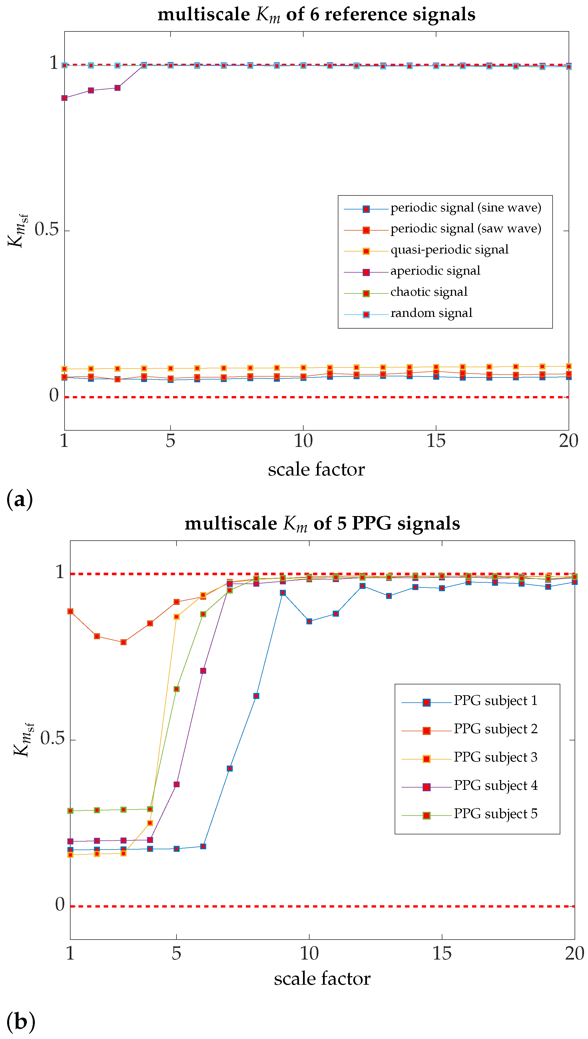
3.2. Reference Signals
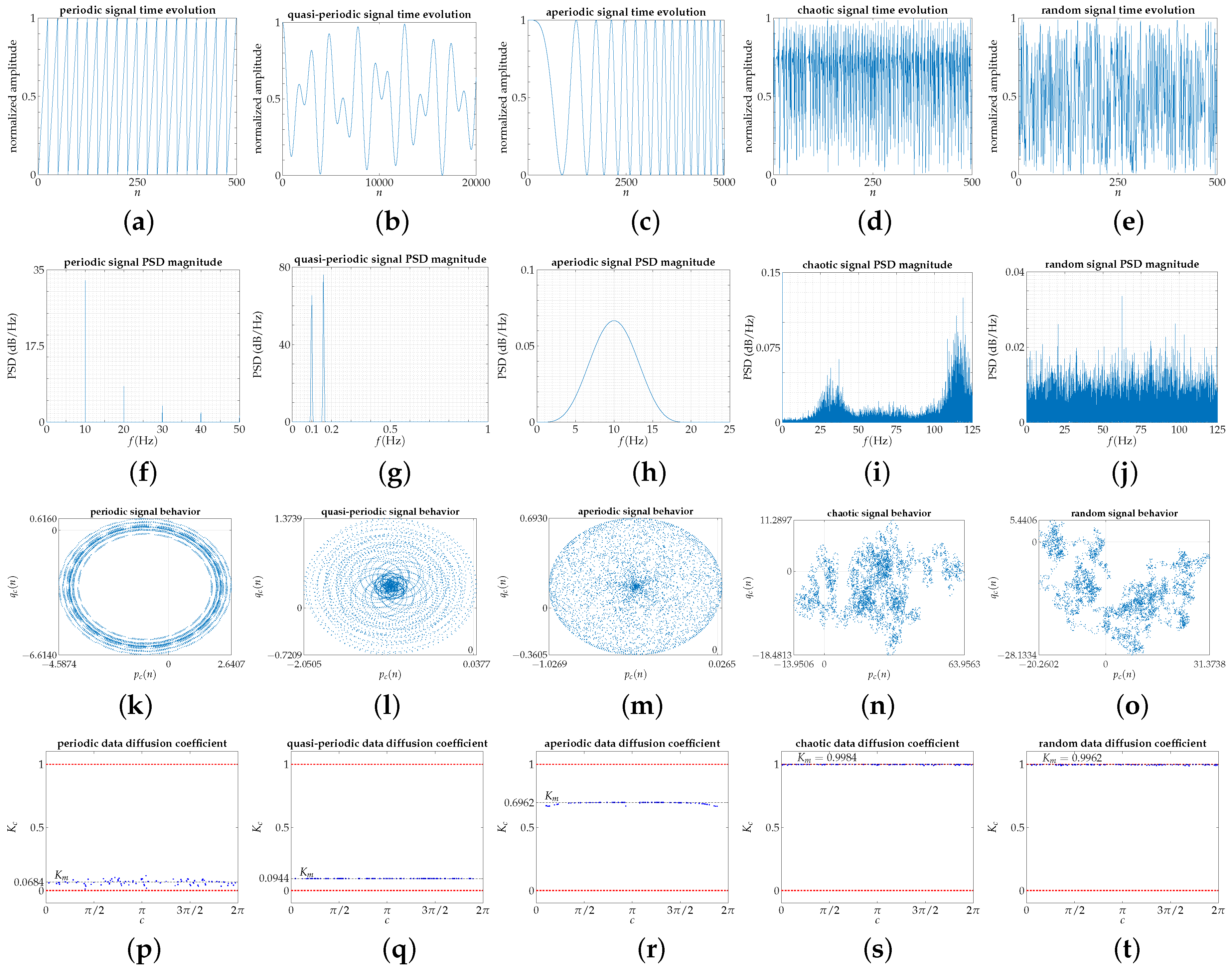
We apply the modified 0–1 test to different signals described below that represent the typical behavior of time series concerning regularity in the repeating patterns of the data. The classification of the signals is according to the order of less to greater complexity, in accordance with the aforementioned approach, from the most regular or periodic evolution to the most random one. Figure 1a–e show the amplitude variation, normalized to the interval [ 0 , 1 ] , of all reference signals in the time domain, and Figure 1f–j represent the Power Spectrum Density (PSD) of all of them.

3.2.1. Periodic

A repetitive pattern occurs and a Fourier series can describe the signal. If a sine wave at f = 10 Hz is analyzed the value of K m 0.06 , say, K m 0 ; to study a more complex signal, with two frequencies whose values are rationally related, we use a saw’s wave at f = 10 Hz:
y periodic ( t ) = 2 t 1 / f 1 2 + t 1 / f .

3.2.2. Quasi-Periodic

A certain recurrence in time evolution may lead to wrongly considering this type of dynamics as an “irregular periodicity” or the same “repetitive structure”. The fact is that the pattern is never repeated if the data have infinite precision, shaping a torus or tori depending on the degrees of freedom [35]. In our case, we apply the most simple one, two cosine waves whose frequencies are irrationally related:
y quasi - periodic ( t ) = cos 1 · t + cos ω 1 · t ,
with ω 1 being the reciprocal of the golden mean, that is, ω 1 = 5 1 / 2 .

3.2.3. Aperiodic

An aperiodic signal has non self-similar repetition even with infinite precision data, although mathematically, it can be considered as a periodic function with an infinite period. The selected function is the one that generates samples by a linear frequency sweeping, the chirp function: f ( t ) = f 0 + k · t , between f 0 = 0 Hz and f 1 = 10 Hz, with k = ( f 1 f 0 ) / T , being T the sweep time.
y aperiodic ( t ) = sin 2 π f 0 t + k 2 t 2 .

3.2.4. Chaotic

The sensitivity of certain deterministic functions to small changes in the initial state is the characteristic footprint of chaotic behavior. The initial uncertainty increases with time, and it is not possible to predict the final state of the system (N. S. Krylov 1944; M. Born 1952) [35]. We use the Hénon map dynamic variable x n , with a = 1.4 y b = 0.3 . The initial conditions were x 0 = y 0 = 0.03 . One hundred thousand samples were generated using the last 60,000 points.
x n + 1 = 1 a x n 2 + y n , y n + 1 = b x n .

3.2.5. Random

It is not deterministic and requires a probabilistic characterization [36]. Sixty thousand points were generated by a uniform distribution in the interval [ 0 , 1 ] .

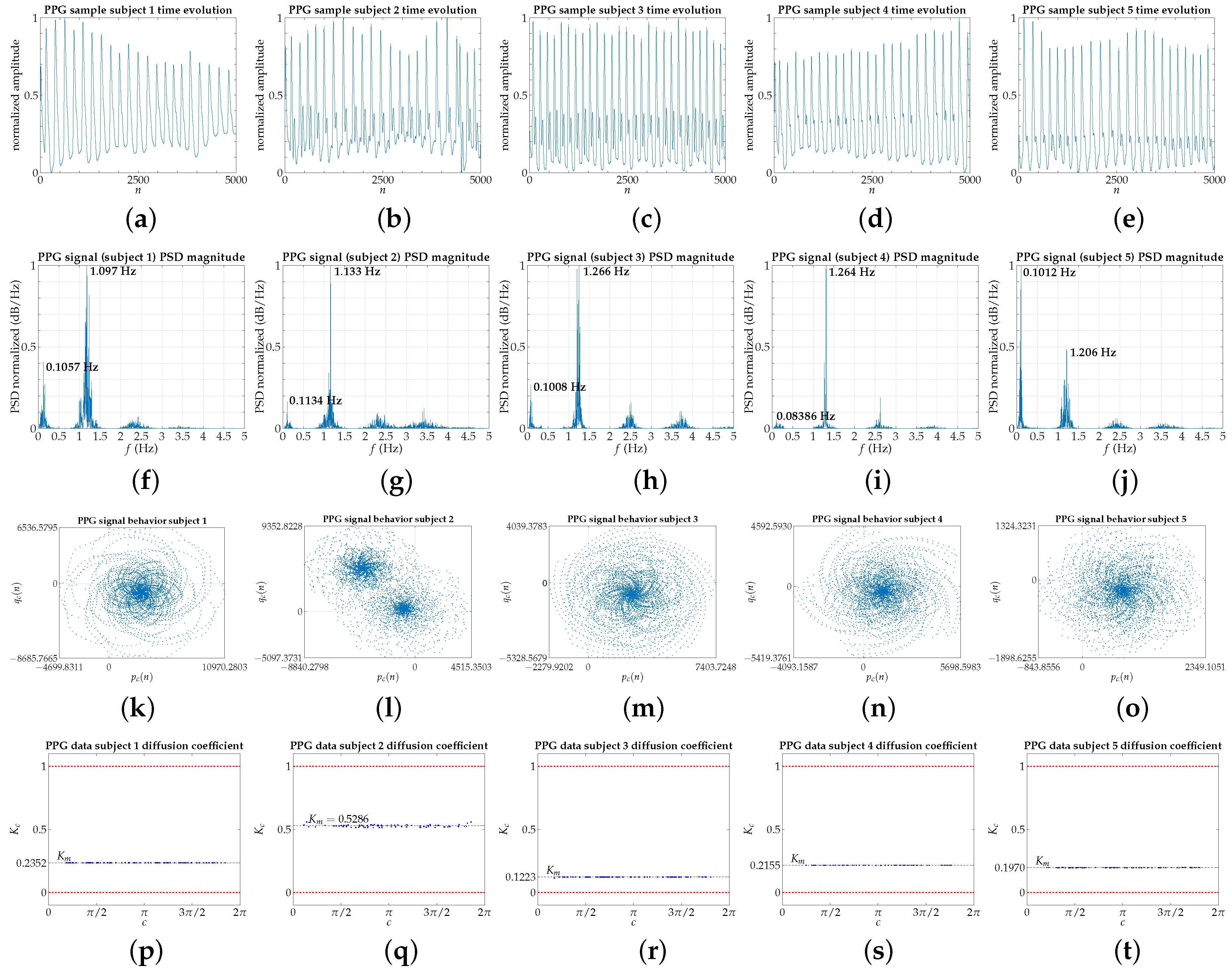
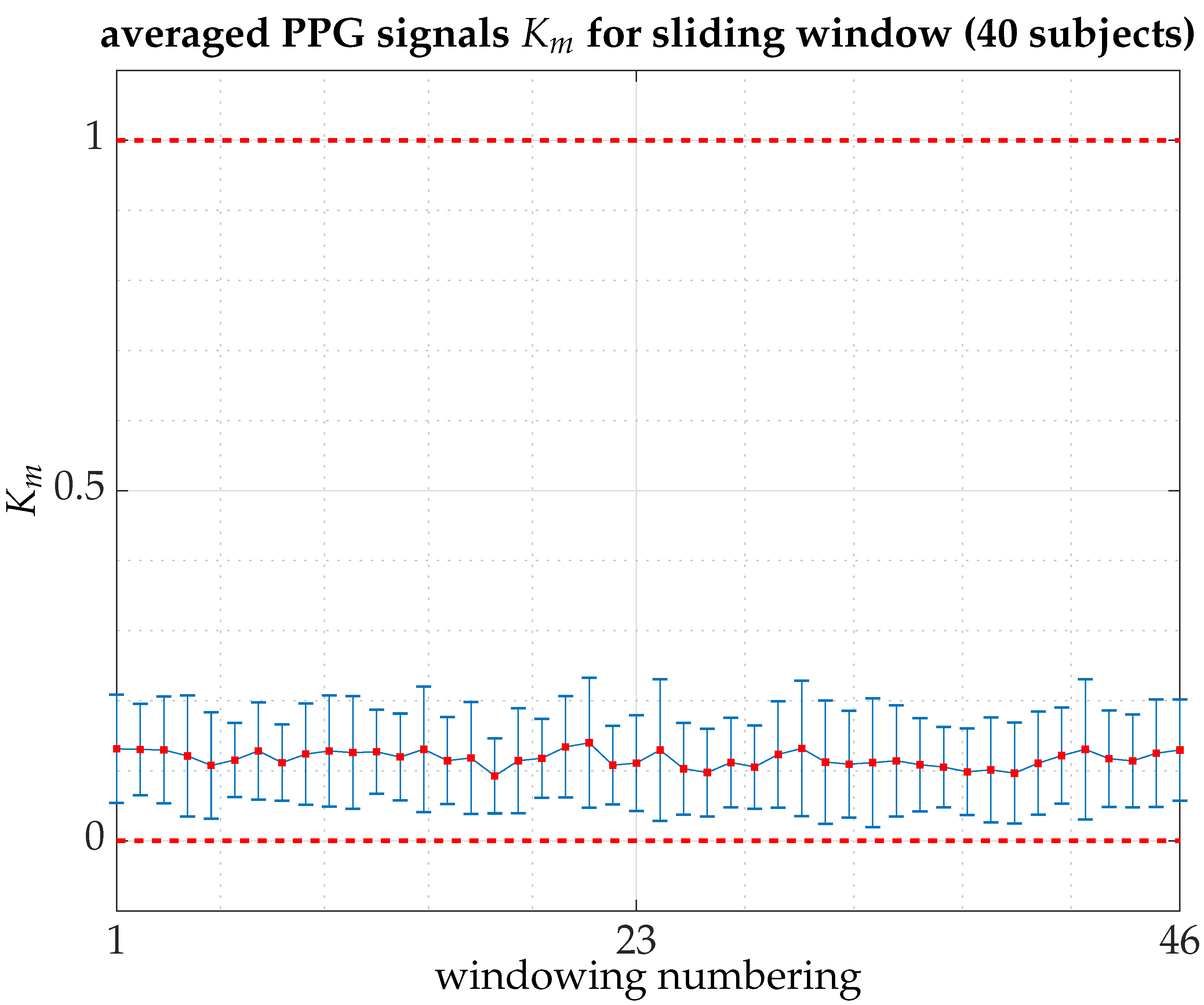
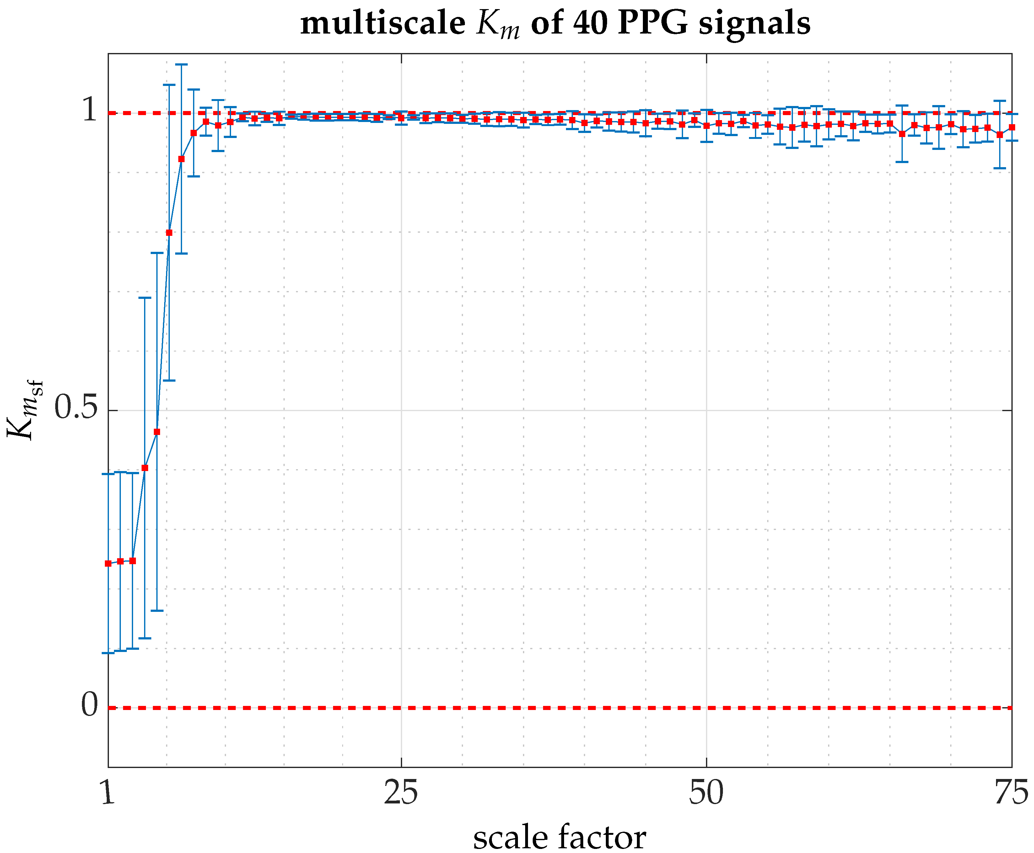
3.3. Biological Signal

This paper focuses only on a single biological signal, the PhotoPlethysmoGraphic (PPG) signal; forward publications will describe the results for more biological signals. We have chosen the PPG signal because it is easily accessible, and the information provided allows us to monitor vital physiological signs [37].

PPG Signal

A pulse oximeter consists of a light emitter and a photodetector that collects and records (pulse or PPG signal) the loss—scattering and absorption—that a beam of light undergoes when it passes through, or is reflected by, a human tissue. It allows detecting blood volume changes in the microvascular bed of tissue—in our case, the middle finger of the left hand—, obtaining valuable information about the cardiovascular system and, on the whole, about the cardiorespiratory system [13]. Given the simplicity of its non-invasive accommodation, in addition to its low cost, a pulse oximeter is very useful in biomedical applications for clinical and sports environments [38]. For a good review, refer to the work of John Allen [39].
In this work, we used forty PPG signals obtained from a national research study in 2015 [27,28]. The project took data from 40 students between 18 and 30 years old and non-regular consumers of psychotropic substances, alcohol, or tobacco. The equipment used to measure all signals is the psychophysiological telemetric system “Rehacor-T” version “Mini” from Medicom MTD Ltd, measuring the PPG signal in the middle finger of the left-hand [27], with a sampling frequency of 250 Hz, say, with sampling time Δ t = 4 ms.
The main body of this paper shows the data of five subjects, illustrating the overall dynamic behavior of the 40 subjects who participated in the experiment (see Appendix A. Accompanying Material). The chosen PPG signals are represented in Figure 2. Depending on the analyzed factor, up to 600,000 points (40 min) were used, those corresponding to the total data recorded in the indicated research project. The results are consistent in the 40 subjects throughout the experimental measurement time of approximately 40 min for each one.
The PPG signal is a complex signal composed of the peripheral pulse synchronized to each heartbeat (AC component of the PPG signal) and modulated by a quasi-DC component that varies slowly due to respiration, vasomotor activity, and vasoconstrictor waves [40]. As we will show later, the mutual coupling between the different components is intricate and operates at different timescales to regulate blood volume based on physiological needs [41,42,43,44]. At small timescales, the regular cardiac rhythm quasi-periodically modulated by the breathing rhythm prevails [37,45,46], as reflected in the two prominent peaks in the PSD of a typical PPG signal, relating to the respiratory, lower frequency peak, and heart, higher frequency peak, rates (see Figure 2f–j).

4. Results and Discussion

As stated earlier, the dynamical analysis of the PPG signal was carried out on 40 young and healthy individuals aged from 18 to 30. However, the main body of this paper only reflects the results of five of them because, in the remaining individuals, the findings are similar (see Figure A1, Figure A2 and Figure A3 in Accompanying Material, Appendix A, for further details).
Figure 1 shows the time and frequency characteristics of reference signals, that is to say, its time evolution and Power Spectrum Density, respectively, along with the modified 0–1 test results, according to Table 1. Power Spectrum Density gives information to distinguish reference signals between them. Time evolution, Figure 1a–e, allows seeing some regularity in the evolutionary structure of the reference signals. The most regular are periodic and quasi-periodic signals, and the most irregular signals are chaotic and random. However, no discernible difference is apparent among the latter signals, even though the chaotic signal is deterministic and the other, the random signal, is not. As time evolves, new frequency components are added to the signal in the case of the aperiodic signal, thereby avoiding its frequency stability. From the spectral view, Figure 1f–j, the periodic signal has a fundamental frequency and harmonics due to the discontinuity present on the dynamic evolution of the signal, resolved with an infinite number of harmonics in Fourier series expansion. The quasi-periodic signal has two visible peaks, whose frequencies are irrationally related. The aperiodic signal is a continuous spectrum in the working frequency range, and the chaotic and random signals display a broadband spectrum; although, in the chaotic signal, it is not uncommon to distinguish some peaks that rise above the broadband baseline.
Concerning the 0–1 test, the diffusion model characterized by the graphic representation of q c ( n ) versus p c ( n ) , Figure 1k–o, describes how the system generating a given signal tries to fill in the surrounding bi-dimensional space. The periodic signal draws up a precise orbit, well-bounded in space; the aperiodic signal covers the entire space bounded by a restrictive area. Conversely, the chaotic and random signals tend to expand erratically by the surrounding space; the dispersion speed is higher for the random signal, according to the coordinate values of the graphic representation, because the chaotic signal is recurring and it usually confirms a clear tendency towards some regions (darker areas) to which it visits most frequently. The quasi-periodic signal presents an intermediate behavior between periodic and aperiodic since it covers the space circumscribed to a restricted area but describing regular paths, in our case elliptical, that do not overlap given the irrational relationship between the constituent frequencies of the signal.
The diffusion correlation coefficient value K m , obtained by applying the modified 0–1 test, according to the procedure proposed in Table 1, is shown for all reference signals in Figure 1p–t. For a periodic signal, K m is tiny ( K m < 0.07 ); in particular, in our case, for our periodic reference signal K m = 0.0684 , and the case of a pure sine wave with a fundamental frequency at 10 Hz K m 0.06 . For a quasi-periodic signal, K m grows very little (≈0.1 or higher) but aiming at an order of magnitude slightly higher; for our quasi-periodic reference signal, K m = 0.0944 . The K m value of the aperiodic signal gets away from the periodic values as new frequencies incorporate into the signal; in our aperiodic reference signal, K m = 0.6962 , when the number of points is 30,000. In the case of a chaotic or random signal K m 1 ; if it is not known a priori, the modified 0–1 test gives the same answer, even knowing that the 0–1 test was initially designed only for deterministic systems.
Figure 2 shows the time evolution, the Power Spectrum Density, and the modified 0–1 test results of PPG signals for five subjects chosen randomly from the 40 students, between 18 and 30 years old and a non-regular consumer of psychotropic substances, alcohol, or tobacco, according to project details [27,28]. Figure 2a–e show directly the PPG signals used for the study, although for visual clarity, only 5000 points of each PPG signal, which correspond to one minute of captured signal, are shown. In Figure 2f–j the PSD of the PPG signals is shown. Two prominent peaks are clearly visible in each PSD, related to the respiratory (lower frequency peak) and heart (higher frequency peak) rates, whose values, irrationally related, are indicated in bold text. Remember PPG fundamental frequency, typically around 1 Hz, depending on heart rate (0.5–4 Hz principal and first harmonic); and respiratory activity in roughly 0.2–0.35 Hz [47]. In any case, all PPG signals have been filtered to avoid motion artifacts as much as possible. The PSD shown for all the subjects in Figure 2f–j are quite similar, except for the relative amplitudes of the maximum peaks.
Further, applying the 0–1 test, we observe in Figure 2k–o that for all of them, the diffusion model characterized by the graphic representation of q c ( n ) versus p c ( n ) , is very similar to that displayed by a quasi-periodic signal, but of a spiral structure similar to a swirl with arms, whose orientation suggests an anti-clockwise or clockwise rotation, with the exception of the individual number 2, where the initial geometric structure seems to unfold into two spirals. In principle, this apparent splitting introduces greater complexity in its dynamics which, as it will be seen below, is reflected in a higher value of K m .
On a small timescale, the K m values for the different PPG signals tend to preserve the quasi-periodic nature (see Figure 2p, and Figure 2r–t) imposed by quasi-periodic modulation of the cardiorespiratory system. When the contribution of other physiological factors pushes the dynamics towards a more aperiodic behavior, as illustrated in Figure 2q, the regulation of blood volume is more effective depending on the physiological needs present and always conditioned by the psychophysical state in which the individual in question is. Hence, each individual externalizes a different K m value within a range of normal operations.
The results summarized in Table 2 also indicate the K m trend, namely, the cumulative effect of K m as the size of the data block increases, starting with a 5000-point data block and in 5000-point incremental steps. So K m is calculated for an initial 5000-point data block, then 10,000, 15,000, and so on up to 60,000 points, taken from the mid-session of the signal acquisition phase. The parameter K m trend allows evaluation of how K m changes as more data are added in the computation of K m ; so somehow, it enables the measurement of new operational modes (very low-frequency components of the PPG signal), as more minutes of the PPG signal are added to the K m analysis. Based on the results of a small timescale analysis of the PPG signal in healthy young people, we can draw that most of the PPG signals have a quasi-periodic behavior [46] (see Figure 3a,b to a complete description). We do not omit to express that several publications provide for a clear linkage between biological signals and quasi-periodic behavior but not with an accurate definition of what is meant by quasi-periodicity property, such as mentioned Ganeshapillai and Guttag [48].
Another relevant result of this work is that as the timescale increases, other factors involved in cardiac rhythm modulation come into play, resulting in a more complex dynamic to subtly enable greater versatility in the cardiac response and, by extension, in the available blood volume at a peripheral level. This more complex dynamic could be chaotic or a preceding behavior, as a transition from a quasi-periodically forced dynamic to a chaotic dynamic via a strange nonchaotic attractor (SNA) [49,50,51,52].
In order to analyze the dynamics of nonlinear coupling on quasi-periodic modulation, we define the multiscale K m K m sf parameter, conceptually inherited from Costa et al. [53], to evaluate how the dynamics of the PPG signal behaves on large timescales. Figure 4a shows how the reference signals preserve a dynamic behavior virtually identical to any scale. However, the findings indicate that on a large timescale, all PPG signals show that K m sf 1 , as illustrated in Figure 4b, may give the idea that the coupling dynamics are chaotic, according to the native 0–1 test. We examine the Maximal Lyapunov Exponent (MLE) and PPG signals’ fractal dimension to confirm this assumption. If a fractal dimension is a fractional number, that is a non-integer number, and the MLE is a positive or negative number. However, very close to zero, the dynamics of the PPG signal, on a large timescale, would a priori resemble the typical behavior of SNAs [52].
PPG signals have not excessively marked fractal character. They always have a Hurst exponent [54] H = 2 D F > 0.5 (see Table 3 for individual results), which attributes to the physiological process a long-term memory (persistence)—in conformity with the low-frequency spectrum of a typical PPG cycle, as Ram et al. clarify [47]; the higher the persistence, the higher the H value. A signal waveform with a considerable value of H involves a smooth time evolution from a geometric perspective.

5. Conclusions

Applying the 0–1 test to the reference signals—periodic, quasi-periodic, aperiodic, chaotic, and random signals—and evaluating a modified version of the test, we show how to describe the dynamics of a biological signal: in our case, the PhotoPlethysmoGraphic (PPG) signal. The analysis has been carried out at different timescales to extract the distinct and relevant dynamics present. Only five subjects are shown in the main body of this paper, while the Accompanying Material (see Appendix A) covers the main results of the 40 subjects that make up the dataset.
With the modified 0–1 test, we described the PPG signal behavior of 40 young, healthy subjects as mainly quasi-periodic on a small timescale. On large timescales, and after conducting a preliminary analysis, we feel that the PPG signals describe a nonchaotic but strange behavior. On a small timescale, the quasi-periodic dynamics imposed by the cardiorespiratory system prevail. Still, on a large timescale, other factors related to the cardiovascular system come into play. These factors force nonlinearly the quasi-periodic dynamics and generate more complex and versatile dynamics that contribute to a heart rate more easily adaptive to changing conditions of the organism in its psychosomatic relationship with the surrounding environment.
So far, on empirical data, the modified 0–1 test does not distinguish between a chaotic signal and a random (stochastic) signal nor does it differentiate between a chaotic signal and the characteristic dynamics of a strange nonchaotic attractor, since both dynamics are aperiodic, due to the fractal nature of its geometric structure. Therefore, the difference between a chaotic attractor and a strange nonchaotic attractor does not meet its geometric structure but rather its dynamic evolution. A (strange) chaotic attractor is characterized by the sensitivity to initial conditions, say, two initially close together trajectories diverge exponentially with time. In the case of a strange nonchaotic attractor, two initially close together trajectories do not diverge exponentially with time, even though each trajectory may have an arbitrarily complex form, so their prediction horizon (predictability) is much wider.
We think that the behavior of the PPG signal, on a large timescale and in the case of healthy young people, is due to the characteristic evolution of a strange nonchaotic attractor, as is shown by the maximal Lyapunov exponents and the Hurst exponents presented in this work.
It is likely that under specific triggers, such as stress situations, the coupling between the different subsystems that make up the cardiorespiratory system will undergo a transition to chaos from a quasi-periodic dynamic. This transition should take place through a strange nonchaotic attractor, as evidenced in different physical [55] and biological systems [56]. Future work will delve into this intriguing bifurcation between regular behavior and presumed chaotic behavior and what physiological consequences could follow from it in the sphere of the PPG signal analysis or indicators related to it.
The PPG signal dynamic behavior analysis moves away from the conventional morphological analysis of the PPG signal, whereby changes in different morphological indicators correlate with cardiovascular disorders and ageing. An accurate characterization of the PPG signal dynamic would allow functional modeling of hemodynamics and peripheral circulation, whatever the physiological peculiarities of each individual. We have indeed used a diffusive model of the PPG signal as a biometric marker, in which the hemodynamic specificity of each individual prevails with time and possible psychophysiological disturbances [57]. It is possible to build wearable devices that, in real-time, will not only authenticate an individual but also anticipate, through the dynamic parameterization of functional models, dynamic symptomatic perturbations of mild dysfunctions, such as stress, or even more severe ones, such as those related to cardiovascular diseases.

Supplementary Materials

The following are available at https://www.mdpi.com/article/10.3390/app11146508/s1, all pictures in Figure 1 and Figure 2: AllFigures1-2.zip.

Author Contributions

Conceptualization, J.d.P.-C. and A.P.G.-M.; methodology, J.d.P.-C.; software, J.d.P.-C.; validation, J.d.P.-C. and A.M.U.; formal analysis, J.d.P.-C. and A.M.U.; data curation, A.M.U.; writing—original draft preparation, J.d.P.-C.; writing—review and editing, J.d.P.-C. and A.P.G.-M.; visualization, J.d.P.-C.; supervision, A.P.G.-M.; project administration, A.M.U.; funding acquisition, A.P.G.-M. All authors have read and agreed to the published version of the manuscript.

Funding

This research received no external funding.

Institutional Review Board Statement

The data used in this study come from the FIS-PI12/00514 project in the Universidad Politécnica de Madrid. It was conducted according to the guidelines of the Declaration of Helsinki, and approved by the Institutional Review Board (or Ethics Committee) of Universidad Politécnica de Madrid (protocol code 2014-16-06 and date of approval 16 July 2014).

Informed Consent Statement

The study includes 40 students from Universidad Politécnica de Madrid (UPM), between age 18 and 30. All signals captured from the middle finger of the left hand and sampled at a frequency of 250 Hz, say, sampling time Δ t = 4 ms. The UPM Ethics Committee approved the study protocol. Participants gave their written informed consent. They were instructed to avoid using any psychotropic substance, alcohol, or tobacco, avoid physical exercise 24 h before each session, get up two hours before starting the sessions, and consume a light breakfast without coffee or tea.

Acknowledgments

The authors would like to thank Life Supporting Technologies Group (LST-UPM) for taking part in project FIS-PI12/00514 from MINECO. Furthermore, the authors gratefully acknowledge the Universidad Politécnica de Madrid (www.upm.es, accessed on 19 March 2021) for providing computing resources on Magerit Supercomputer. Following the same line, the authors want to thank especially the support given by Raúl Durán Díaz, from the Universidad de Alcalá (UAH) and the Spanish National Research Council (CSIC), providing a cluster of servers with which to execute some of the preliminary computational algorithmic tests of this work. The cluster consists of ten computing nodes, with a total of 64 cores, an Intel Xeon architecture, and 166 GB of memory. Finally, the authors would like to thank the referees for their useful comments.

Conflicts of Interest

The authors declare no conflict of interest.

Appendix A. Accompanying Material

Figure A1. Averaged K m for the 40 subjects (PPG signals) that make up the pilot experiment, over 150,000 points (10 min at the halfway point in between the beginning and the completion of the experimental session) in windows of 15,000 points with overlapping of 80% [computation time for all signals on Magerit Supercomputer, a server cluster consisting of 68 Lenovo ThinkSystem SD530 nodes each with 2 × 20-core Intel Xeon Gold 6230 processors at 2.10 GHz (1344 GFLOPS), 192 GB of RAM and 480 GB of local SSD: 70 h 28 min and 27 s]. The graph shows the averaged values of K m in each window (46 windows in total) together with error bars indicating the standard deviation. The average value of K m over all windows is 0.1173 with a standard deviation of ± 0.0114 .
Applsci 11 06508 g0a1
Figure A2. The parameter K m trend for the 40 subjects (PPG signals) that make up the pilot experiment [computation time for all signals on Magerit Supercomputer, a server cluster consisting of 68 Lenovo ThinkSystem SD530 nodes each with 2 × 20-core Intel Xeon Gold 6230 processors at 2.10 GHz (1344 GFLOPS), 192 GB of RAM and 480 GB of local SSD: 117 h 14 min and 30 s]. At each iteration, the block size is increased by an additional 15,000 points until a total of 150,000 points is reached. The graph shows the averaged values of K m in each block of increasing size (10 blocks in total) together with error bars indicating the standard deviation. On average, PPG signals undergo an upward drift as more data are added while remaining within a dynamic regime more consistent with quasi-periodic behavior.
Applsci 11 06508 g0a2
Figure A3. The multiscale K m K m sf for the 40 subjects (PPG signals) that make up the pilot experiment [computation time for all signals on Magerit Supercomputer, a server cluster consisting of 68 Lenovo ThinkSystem SD530 nodes each with 2 × 20-core Intel Xeon Gold 6230 processors at 2.10 GHz (1344 GFLOPS), 192 GB of RAM and 480 GB of local SSD: 25 h 51 min and 4 s]. The graph shows the averaged values of K m sf value for each scale factor over a time horizon of 10 s (150,000 points) and 75 scale factors, together with error bars indicating the standard deviation. On average, PPG signals show a clear dynamic transition with a trend to a K m sf 1 on large timescales. In the absence of more in-depth analysis, we hypothesize that the high dynamic variability on small timescales subordinate to the psychosomatic deviations of the individuals who participated in the experiment. Some individuals were already more excited (stressed) than others because they knew they were participating in a study or because of personal circumstances beyond our knowledge. As the scale factor increases, the low-frequency dynamic coupling that regulates the cardiovascular system comes into play within normal operating ranges, with low variability. However, at very low frequency, the dynamic variability increases, yet it is not very pronounced. There is a statistical bias due to the unavailability of sufficient data or artifacts that could not be removed or going further to our lack of knowledge concerning subsystems coupled in the regulation process.
Applsci 11 06508 g0a3

References

  1. Seely, A.J.E.; Macklem, P. Fractal variability: An emergent property of complex dissipative systems. Chaos Interdiscip. J. Nonlinear Sci. 2012, 22, 013108. [Google Scholar] [CrossRef]
  2. Hertzman, A.B. Photoelectric Plethysmography of the Fingers and Toes in Man. Exp. Biol. Med. 1937, 37, 529–534. [Google Scholar] [CrossRef]
  3. Murray, W.B.; Foster, P.A. The peripheral pulse wave: Information overlooked. J. Clin. Monit. 1996, 12, 365–377. [Google Scholar] [CrossRef] [PubMed]
  4. Goh, C.H.; Tan, L.K.; Lovell, N.H.; Ng, S.C.; Tan, M.P.; Lim, E. Robust PPG motion artifact detection using a 1-D convolution neural network. Comput. Methods Programs Biomed. 2020, 196, 105596. [Google Scholar] [CrossRef] [PubMed]
  5. Liu, S.H.; Li, R.X.; Wang, J.J.; Chen, W.; Su, C.H. Classification of Photoplethysmographic Signal Quality with Deep Convolution Neural Networks for Accurate Measurement of Cardiac Stroke Volume. Appl. Sci. 2020, 10, 4612. [Google Scholar] [CrossRef]
  6. Cannesson, M.; Talke, P. Recent advances in pulse oximetry. F1000 Med. Rep. 2009, 1. [Google Scholar] [CrossRef] [PubMed] [Green Version]
  7. Lee, J.; Kim, M.; Park, H.K.; Kim, I.Y. Motion Artifact Reduction in Wearable Photoplethysmography Based on Multi-Channel Sensors with Multiple Wavelengths. Sensors 2020, 20, 1493. [Google Scholar] [CrossRef] [PubMed] [Green Version]
  8. Seok, D.; Lee, S.; Kim, M.; Cho, J.; Kim, C. Motion Artifact Removal Techniques for Wearable EEG and PPG Sensor Systems. Front. Electron. 2021, 2. [Google Scholar] [CrossRef]
  9. Kim, B.; Yoo, S. Motion Artifact Reduction in Photoplethysmography Using Independent Component Analysis. IEEE Trans. Biomed. Eng. 2006, 53, 566–568. [Google Scholar] [CrossRef]
  10. Hanyu, S.; Xiaohui, C. Motion artifact detection and reduction in PPG signals based on statistics analysis. In Proceedings of the IEEE 2017 29th Chinese Control And Decision Conference (CCDC), Chongqing, China, 28–30 May 2017. [Google Scholar] [CrossRef]
  11. Majeed, I.A.; Jos, S.; Arora, R.; Choi, K.; Bae, S. Motion Artifact Removal of Photoplethysmogram (PPG) Signal. In Proceedings of the 2019 41st Annual International Conference of the IEEE Engineering in Medicine and Biology Society (EMBC), Berlin, Germany, 23–27 July 2019. [Google Scholar] [CrossRef]
  12. Pollreisz, D.; TaheriNejad, N. Detection and Removal of Motion Artifacts in PPG Signals. Mob. Netw. Appl. 2019. [Google Scholar] [CrossRef] [Green Version]
  13. Tamura, T. Current progress of photoplethysmography and SPO2 for health monitoring. Biomed. Eng. Lett. 2019, 9, 21–36. [Google Scholar] [CrossRef]
  14. Islam, T.T.; Ahmed, M.S.; Hassanuzzaman, M.; Amir, S.A.B.; Rahman, T. Blood Glucose Level Regression for Smartphone PPG Signals Using Machine Learning. Appl. Sci. 2021, 11, 618. [Google Scholar] [CrossRef]
  15. Cosoli, G.; Iadarola, G.; Poli, A.; Spinsante, S. Learning classifiers for analysis of Blood Volume Pulse signals in IoT-enabled systems. In Proceedings of the 2021 IEEE International Workshop on Metrology for Industry 4.0 & IoT, Roma, Italy, 7–9 June 2021. [Google Scholar]
  16. Cosoli, G.; Scalise, L.; Poli, A.; Spinsante, S. Wearable devices as a valid support for diagnostic excellence: Lessons from a pandemic going forward. Health Technol. 2021, 11, 673–675. [Google Scholar] [CrossRef] [PubMed]
  17. Sprott, J.C. Chaos and Time-Series Analysis; Oxford University Press: New York, NY, USA, 2003. [Google Scholar]
  18. Kantz, H.; Schreiber, T. Nonlinear Time Series Analysis, 2nd ed.; Cambridge Nonlinear Science Series; Cambridge University Press: Cambridge, UK, 2004. [Google Scholar]
  19. Tsonis, A.A. Chaos: From Theory to Applications; Springer: New York, NY, USA, 2012. [Google Scholar]
  20. Toker, D.; Sommer, F.T.; D’Esposito, M. A simple method for detecting chaos in nature. Commun. Biol. 2020, 3. [Google Scholar] [CrossRef] [Green Version]
  21. Bhattacharya, J.; Kanjilal, P.P.; Muralidhar, V. Analysis and characterization of photo-plethysmographic signal. IEEE Trans. Biomed. Eng. 2001, 48, 5–11. [Google Scholar] [CrossRef] [PubMed]
  22. Martin-Martinez, D.; de-la Higuera, P.C.; Martin-Fernandez, M.; Alberola-Lopez, C. Stochastic Modeling of the PPG Signal: A Synthesis-by-Analysis Approach With Applications. IEEE Trans. Biomed. Eng. 2013, 60, 2432–2441. [Google Scholar] [CrossRef]
  23. Sviridova, N.; Zhao, T.; Aihara, K.; Nakamura, K.; Nakano, A. Photoplethysmogram at green light: Where does chaos arise from? Chaos Solitons Fractals 2018, 116, 157–165. [Google Scholar] [CrossRef]
  24. Gottwald, G.A.; Melbourne, I. A new test for chaos in deterministic systems. Proc. R. Soc. A Math. Phys. Eng. Sci. 2004, 460, 603–611. [Google Scholar] [CrossRef] [Green Version]
  25. de Pedro-Carracedo, J.; Fuentes-Jimenez, D.; Ugena, A.M.; Gonzalez-Marcos, A.P. Phase Space Reconstruction from a Biological Time Series: A Photoplethysmographic Signal Case Study. Appl. Sci. 2020, 10, 1430. [Google Scholar] [CrossRef] [Green Version]
  26. Czegledy, F.; Katz, J. Biological systems: Stochastic, deterministic or both. Open Syst. Inf. Dyn. 1995, 3, 179–188. [Google Scholar] [CrossRef]
  27. Aguiló, J.; Ferrer-Salvans, P.; García-Rozo, A.; Armario, A.; Corbi, A.; Cambra, F.J.; Bailón, R.; González-Marcos, A.; Caja, G.; Aguiló, S.; et al. Project ES3: Attempting to quantify and measure the level of stress. Rev. Neurol. 2015, 61, 405–415. [Google Scholar]
  28. Arza, A.; Garzón-Rey, J.M.; Lázaro, J.; Gil, E.; López-Antón, R.; de la Cámara, C.; Laguna, P.; Bailón, R.; Aguiló, J. Measuring acute stress response through physiological signals: Towards a quantitative assessment of stress. Med. Biol. Eng. Comput. 2018, 57, 271–287. [Google Scholar] [CrossRef] [Green Version]
  29. Gottwald, G.A.; Melbourne, I. Testing for chaos in deterministic systems with noise. Phys. D Nonlinear Phenom. 2005, 212, 100–110. [Google Scholar] [CrossRef] [Green Version]
  30. Gottwald, G.A.; Melbourne, I. Comment on “Reliability of the 0–1 test for chaos”. Phys. Rev. E 2008, 77. [Google Scholar] [CrossRef] [Green Version]
  31. Skokos, C.; Gottwald, G.A.; Laskar, J. Chaos Detection and Predictability; Lecture Notes in Physics; Springer: Berlin/Heidelberg, Germany, 2016. [Google Scholar]
  32. Gottwald, G.A.; Melbourne, I. On the validity of the 0–1 test for chaos. Nonlinearity 2009, 22, 1367–1382. [Google Scholar] [CrossRef]
  33. Grassberger, P. Toward a quantitative theory of self-generated complexity. Int. J. Theor. Phys. 1986, 25, 907–938. [Google Scholar] [CrossRef]
  34. Badii, R.; Politi, A.; Remo, B. Complexity; Cambridge University Press: Cambridge, UK, 2003. [Google Scholar]
  35. Landau, L.D.; Lifshitz, E.M. Fluid Mechanics, 2nd ed.; Pergamon Press: Oxford, UK, 1987. [Google Scholar]
  36. Enderle, J.; Bronzino, J. Introduction to Biomedical Engineering, 3rd ed.; Biomedical Engineering; Elsevier Science: Burlington, MA, USA, 2011. [Google Scholar]
  37. Chen, M.; Zhu, Q.; Wu, M.; Wang, Q. Modulation Model of the Photoplethysmography Signal for Vital Sign Extraction. IEEE J. Biomed. Health Inform. 2021, 25, 969–977. [Google Scholar] [CrossRef]
  38. Mendes, J.J.A., Jr.; Vieira, M.E.M.; Pires, M.B.; Stevan, S.L., Jr. Sensor Fusion and Smart Sensor in Sports and Biomedical Applications. Sensors 2016, 16, 1569. [Google Scholar] [CrossRef] [PubMed]
  39. Allen, J. Photoplethysmography and its application in clinical physiological measurement. Physiol. Meas. 2007, 28, R1–R39. [Google Scholar] [CrossRef] [PubMed] [Green Version]
  40. Meredith, D.J.; Clifton, D.; Charlton, P.; Brooks, J.; Pugh, C.W.; Tarassenko, L. Photoplethysmographic derivation of respiratory rate: A review of relevant physiology. J. Med. Eng. Technol. 2011, 36, 1–7. [Google Scholar] [CrossRef] [Green Version]
  41. Glass, L. Multistable spatiotemporal patterns of cardiac activity. Proc. Natl. Acad. Sci. USA 2005, 102, 10409–10410. [Google Scholar] [CrossRef] [Green Version]
  42. Goldberger, A.L. Giles F. Filley Lecture. Complex Systems. Proc. Am. Thorac. Soc. 2006, 3, 467–471. [Google Scholar] [CrossRef] [PubMed] [Green Version]
  43. Wessel, N.; Riedl, M.; Kurths, J. Is the normal heart rate “chaotic” due to respiration? Chaos Interdiscip. J. Nonlinear Sci. 2009, 19, 028508. [Google Scholar] [CrossRef] [PubMed]
  44. Bartsch, R.P.; Schumann, A.Y.; Kantelhardt, J.W.; Penzel, T.; Ivanov, P.C. Phase transitions in physiologic coupling. Proc. Natl. Acad. Sci. USA 2012, 109, 10181–10186. [Google Scholar] [CrossRef] [Green Version]
  45. Khreis, S.; Ge, D.; Carrault, G. Estimation of Breathing Rate From the Photoplethysmography Using Respiratory Quality Indexes. In Proceedings of the 2018 Computing in Cardiology Conference (CinC), Maastricht, The Netherlands, 23–26 September 2018; Volume 45, pp. 1–4. [Google Scholar] [CrossRef]
  46. Pedro-Carracedo, J.D.; Fuentes-Jimenez, D.; Ugena, A.M.; Gonzalez-Marcos, A.P. Is the PPG Signal Chaotic? IEEE Access 2020, 8, 107700–107715. [Google Scholar] [CrossRef]
  47. Ram, M.R.; Madhav, K.V.; Krishna, E.H.; Komalla, N.R.; Reddy, K.A. A Novel Approach for Motion Artifact Reduction in PPG Signals Based on AS-LMS Adaptive Filter. IEEE Trans. Instrum. Meas. 2012, 61, 1445–1457. [Google Scholar] [CrossRef]
  48. Ganeshapillai, G.; Guttag, J. Real time reconstruction of quasiperiodic multi parameter physiological signals. EURASIP J. Adv. Signal Process. 2012, 2012. [Google Scholar] [CrossRef] [Green Version]
  49. Grebogi, C.; Ott, E.; Pelikan, S.; Yorke, J.A. Strange attractors that are not chaotic. Phys. D Nonlinear Phenom. 1984, 13, 261–268. [Google Scholar] [CrossRef]
  50. Brindley, J.; Kapitaniak, T. Existence and characterization of strange nonchaotic attractors in nonlinear systems. Chaos Solitons Fractals 1991, 1, 323–337. [Google Scholar] [CrossRef]
  51. Pikovsky, A.S.; Feudel, U. Characterizing strange nonchaotic attractors. Chaos Interdiscip. J. Nonlinear Sci. 1995, 5, 253–260. [Google Scholar] [CrossRef]
  52. Prasad, A.; Negi, S.S.; Ramaswamy, R. Strange Nonchaotic Attractors. Int. J. Bifurc. Chaos 2001, 11, 291–309. [Google Scholar] [CrossRef] [Green Version]
  53. Costa, M.; Goldberger, A.L.; Peng, C.K. Multiscale entropy analysis of biological signals. Phys. Rev. E 2005, 71, 021906. [Google Scholar] [CrossRef] [Green Version]
  54. Hurst, H.E. Long-Term Storage of Reservoirs: An Experimental Study. Trans. Am. Soc. Civ. Eng. 1951, 116, 770–799. [Google Scholar] [CrossRef]
  55. Zhou, T.; Moss, F.; Bulsara, A. Observation of a strange nonchaotic attractor in a multistable potential. Phys. Rev. A 1992, 45, 5394–5400. [Google Scholar] [CrossRef] [PubMed] [Green Version]
  56. Ding, M.; Kelso, J.A.S. Phase-resetting map and the dynamics of quasi-periodically forced biological oscillators. Int. J. Bifurc. Chaos 1994, 4, 553–567. [Google Scholar] [CrossRef]
  57. de Pedro-Carracedo, J.; Fuentes-Jimenez, D.; Ugena, A.M.; Gonzalez-Marcos, A.P. Transcending conventional biometry frontiers: Diffusive Dynamics PPG Biometry. arXiv 2020, arXiv:2007.15060. [Google Scholar]
Figure 1. (These pictures are made available for downloading in Supplementary Materials.) Each column corresponds with a reference signal: periodic, quasi-periodic, aperiodic, chaotic, and random. (ae) Time evolution with amplitude normalized to the interval [ 0 , 1 ] . For visual clarity in each signal, the interval that best identifies its time structure is chosen; (fj) Power Spectrum Density (PSD); (ko) Representation of Equation (1) for c = 2.5 , with N = 5000 points; (pt) K m results of the modified 0–1 test, for 100 random c values, with correlation method.
Applsci 11 06508 g001
Figure 2. (These pictures are made available for downloading in Supplementary Materials.) Each column corresponds with a subject (five individuals chosen randomly); the number of points: 30,000. (ae) PPG signals, with amplitude normalized to the interval [ 0 , 1 ] —for visual clarity, only 5000 points of each PPG signal are shown; (fj) Power Spectrum Density (PSD). Two prominent peaks are clearly visible in each PSD, related to the respiratory (lower frequency peak) and heart (higher frequency peak) rates, whose values are indicated in bold text; (ko) Representation of Equation (1) for c = 2.5 , with N = 5000 points; (pt) K m results of the modified 0–1 test, for 100 random c values, with correlation method.
Applsci 11 06508 g002
Figure 3. The parameter K m trend for several reference signals, as well as for PPG signals, acquired from five individuals chosen at random [computation time per signal in a server cluster consisting of 10 computing nodes, with a total of 64 cores and Intel Xeon architecture, and 166 GB of memory: 17 h 7 min and 7 s]. (a) K m trend for two periodic signals, one quasi-periodic signal, one aperiodic signal, one chaotic signal, and a random signal; as shown in the figure, only the aperiodic signal displays a notable increasing trend as more points are added in the computation of K m ; (b) PPG samples (five individuals chosen at random). With the exception of PPG subject 2, which shows a clear trend towards likely aperiodic behavior, in all other respects, a slight drift remains within a dynamic regime closer to the quasi-periodic behavior.
Applsci 11 06508 g003
Figure 4. The multiscale K m K m sf for several reference signals, as well as for PPG signals, acquired from five individuals chosen at random [computation time per signal in a server cluster consisting of 10 computing nodes, with a total of 64 cores and Intel Xeon architecture, and 166 GB of memory: 6 h 7 min and 7 s]. (a) Multiscale K m for two periodic signals, one quasi-periodic signal, one aperiodic signal, one chaotic signal, and a random signal; almost all the signals have recurrent dynamics at all different scales; (b) PPG samples (five individuals chosen at random). All of them, regardless of their dynamics on a small timescale, trend to a K m sf 1 on a large timescale.
Applsci 11 06508 g004
Table 1. Steps of the (modified) 0–1 test algorithm.
Step 1: From Equation (1) Resolve: p c ( n ) and q c ( n ) , n = 1 , 2 , , N ; c ( 0 , 2 π ) Number of
observations: N
Plots: Figure 1k–o,
Figure 2k–o
Step 2: Analyze the diffusive, or non-diffusive, behavior of p c ( n ) and q c ( n )
M c ( n ) = 1 N j = 1 N n [ p c ( j + n ) p c ( j ) ] 2 +      [ q c ( j + n ) q c ( j ) ] 2 , n = 1 , 2 , 3 ,
n N 0 N The plot of this step is not relevant in this work
Step 3: Grown rate K c Regression or correlation method
Step 4: Steps 1–3 must be executed for various values of c (randomly selected) In practice, 100 choices of c ( 0 , 2 π ) are sufficient; moreover, in our case, K m = median ( K c ) once outliers of K c have been removed Plots: Figure 1p–t,
Figure 2p–t
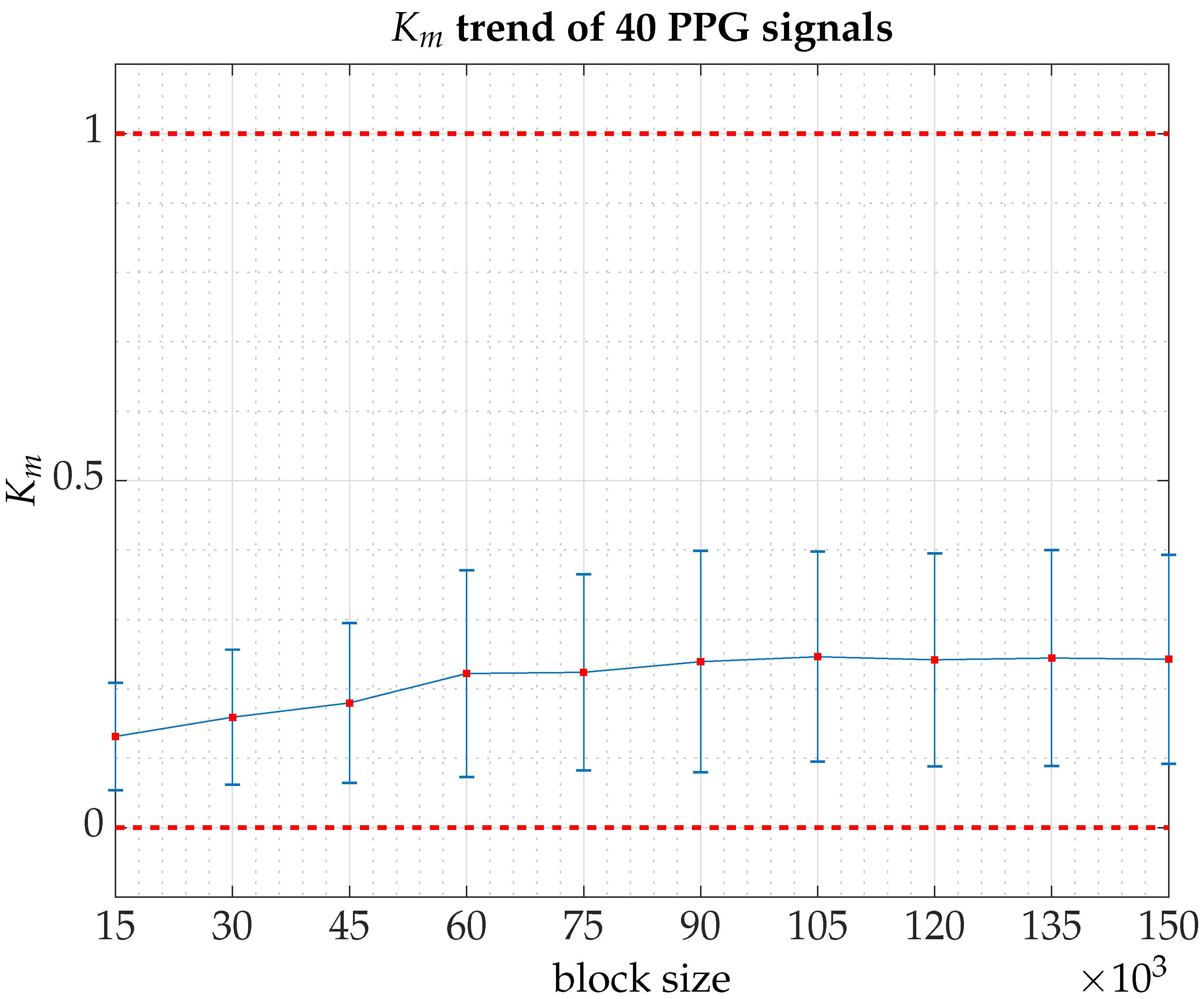
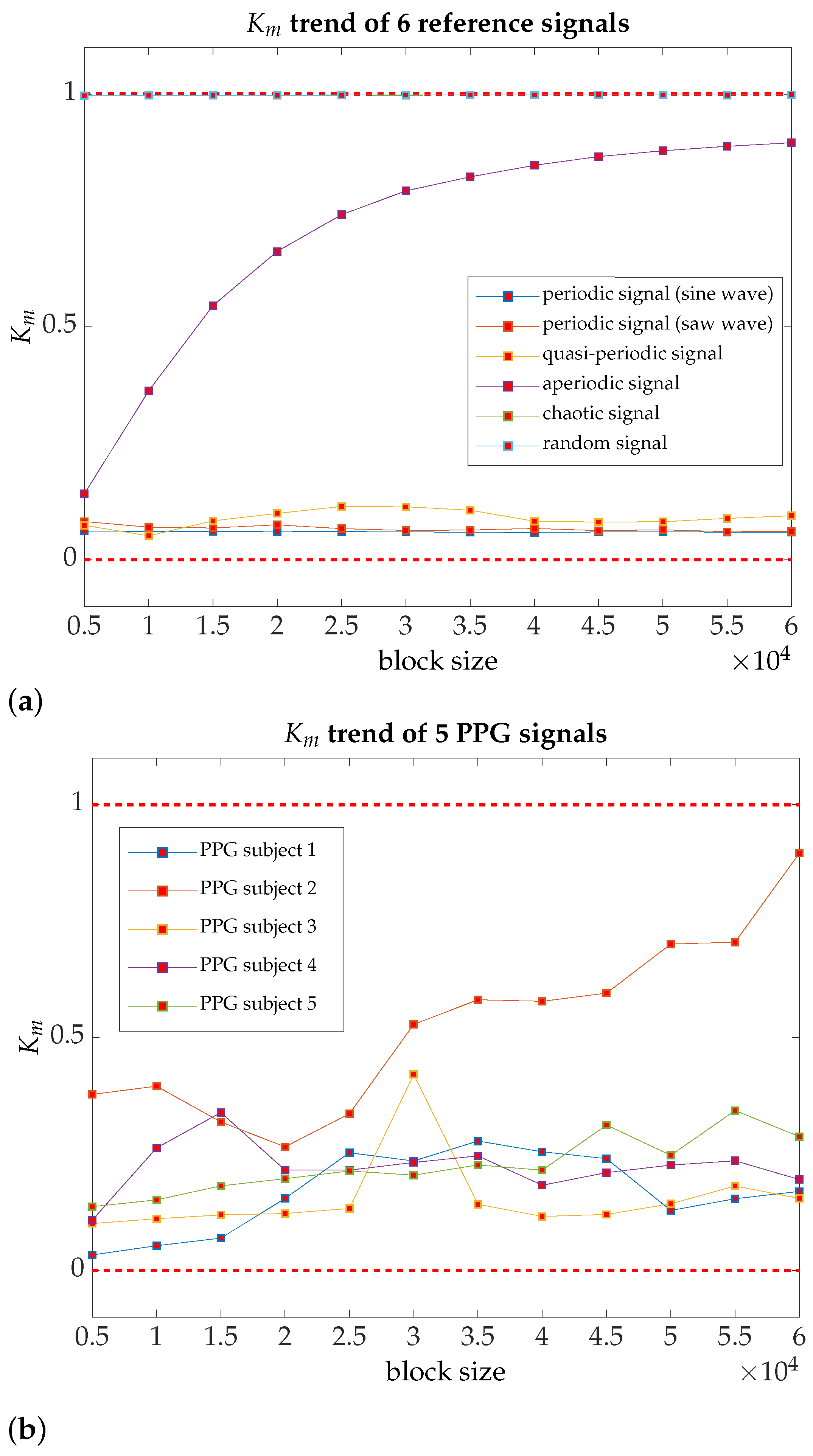
Table 2. Averaged K m over 600,000 points (40 min) [computation time per signal in a server cluster consisting of 10 computing nodes, with a total of 64 cores and Intel Xeon architecture, and 166 GB of memory: 37 h 18 min and 11 s], over 150,000 points (10 min at a half-way point in between the beginning and the completion of the experimental session) in windows of 30,000 points with an overlapping of 50% and the K m trend from a block size of 5000 points to a block size of 60,000 points in increments of 5000 points (4 min at a half-way point in between the beginning and the completion of the experimental session), of the PPG signals, acquired from five individuals chosen at random.
Evaluated SignalAveraged K m
(600,000 Points)
Averaged K m
(150,000 Points)
K m Trend
(up to 60,000 Points )
K m σ K m σ K m
subject number 1 (PPG1) 0.1318 ± 0.0724 0.3330 ± 0.0410 0.1697
subject number 2 (PPG2) 0.2426 ± 0.1946 0.3705 ± 0.0502 0.8959
subject number 3 (PPG3) 0.1784 ± 0.0865 0.1619 ± 0.0236 0.1548
subject number 4 (PPG4) 0.1268 ± 0.0613 0.2602 ± 0.0274 0.1953
subject number 5 (PPG5) 0.1464 ± 0.0969 0.2798 ± 0.0261 0.2873
Table 3. Maximal Lyapunov exponent ( λ m a x ) and fractal dimension ( D F ), of the PPG signals, acquired from five individuals chosen at random.
Evaluated SignalMaximal Lyapunov Exponent (MLE)Fractal Dimension
λ max D F
subject number 1 (PPG1) 0.0254 1.1168
subject number 2 (PPG2) 0.0488 1.1937
subject number 3 (PPG3) 0.0290 1.2112
subject number 4 (PPG4) + 0.0002 1.1730
subject number 5 (PPG5) 0.0419 1.1655
Publisher’s Note: MDPI stays neutral with regard to jurisdictional claims in published maps and institutional affiliations.

