Article

Ultrasonic Array Imaging of Nuclear Austenitic V-Shape Welds with Inhomogeneous and Unknown Anisotropic Properties

by
Corentin Menard
1,
Sébastien Robert
1,* and
Dominique Lesselier
2
1
Paris-Saclay University, CEA, List, 91191 Palaiseau, France
2
Laboratoire des Signaux et Systèmes, Paris-Saclay University, CNRS, CentraleSupélec, 91190 Gif-sur-Yvette, France
*
Author to whom correspondence should be addressed.
Appl. Sci. 2021, 11(14), 6505; https://doi.org/10.3390/app11146505
Submission received: 31 May 2021 / Revised: 21 June 2021 / Accepted: 22 June 2021 / Published: 15 July 2021

Abstract

:
The quality of ultrasound images of welds is highly penalized by the dendritic structure of the material that forms during cooling. The image of a flaw is all the more degraded as a reliable description of such a medium is most of the time not possible, due to the poor knowledge on the weld at time of inspection. In a previous work, we demonstrated the efficiency of an optimization procedure to correct a degraded Total Focusing Method (TFM) image of a point-like reflector inside a homogeneous weld, with uniaxial grain orientation. In the present contribution, this procedure is extended to more realistic welds with a varying grain orientation, and it is evaluated with a 64-element array emitting at 5 MHz on stainless steel weld samples featuring side-drilled holes of 1 mm diameter. A first proof of concept with simulated echoes, and then two experiments show that defects that were hardly visible on TFM images before the optimization are now well reconstructed and with positioning errors inferior to 1 mm.

1. Introduction

Ultrasonic phased array inspections are increasingly used in Non-Destructive Testing (NDT) for their high performances in flaw detection, material characterization and imaging [1]. Among them, one well-known imaging technique is the Total Focusing Method (TFM) [2]: it consists of synthetically focusing the inter-element signals recorded with an array on every point of the region of interest using a “delay-and-sum” strategy. The recorded signals then physically correspond to the inter-elements impulse responses of the medium [3,4]. Therefore, the TFM imaging is simply applied a posteriori, without enforcing delay laws during the acquisition, and one of the advantages of this method is thus that any enhancement or modification can be achieved in a post-processing step [5,6].
In the case of austenitic welds, the quality of the reconstructed TFM image highly depends on the accuracy of the weld model to describe the waves’ propagation in the material. During the welding process, the cooling of the fusion zone is governed by various phenomena (heat and fluid flows, vaporization and solidification, gasses dissolution, strong mechanical and heat strains, matter re-melting, etc.) that lead to a dendritic growth of the matter with primary and secondary arms [7,8]. It is therefore difficult to precisely predict or estimate the complex 3D-varying weld properties. Moreover, a characterization of the material is often not available at the time of inspection and little information is known to provide a reliable weld model. As a result, when the numerical description is not close enough to the actual material properties, the computed TFM image can be severely degraded.
In a previous study, we presented an optimization procedure to increase the quality of TFM images of point-like defects in unknown anisotropic and homogeneous steel-based components [9]. The procedure operates by varying the parameters of the model that describes the weld, by means of an optimization algorithm, until no further increase in the maximum amplitude of the defect echo. In the current contribution, we extend the optimization procedure to deal with unknown and inhomogeneous austenitic welds as encountered in nuclear power plants.
This paper is organized as follows: in Section 2, we recall the different steps of the optimization procedure with details on the Ogilvy’s weld model, used herein, and the particle swarm algorithm to which has been added a warm restart strategy; in Section 3, we then evaluate the optimization procedure with a numerical proof of concept; and in Section 4, the procedure is experimentally evaluated with austenitic weld samples containing artificial defects located either in the middle of the weld or on its chamfer.

2. The Optimization Procedure

In this section, we recall the principle of the optimization procedure designed in [9] for improving 2D ultrasonic imaging in welds. Then, the Ogilvy’s model used hereafter to describe the continuously variable grain orientation of the weld is recalled. Finally, some details are given on the swarm particle algorithm, which has been upgraded with a warm restart strategy, and that performs the optimization.

2.1. Principle of the TFM-Based Optimization

Based on a single acquisition of the inter-element impulse responses with a linear array, the optimization procedure enhances the quality of a TFM image with an iterative algorithm that modifies the weld model parameters accordingly to increase the amplitude of the defect echo [9]. Only the propagation of Quasi-Longitudinal (QL) waves is considered to form the images. The procedure is divided into four main steps:
  • Computation of N propagation times for each pixel of the image, where N is the number of array elements;
  • Computation of the TFM image by coherent summation of the N2 inter-element signals at each pixel;
  • Extraction of the image quality criterion (maximum amplitude of the defect echo—Amax);
  • Modification of the weld model parameters.
The computation of the propagation times is achieved with the semi-analytical ray-tracing algorithm of the CIVA software [10,11]. We encourage the readers to refer to [9] for more information on the procedure.
The main assets of our approach are that, unlike other approaches, it does not rely on any foreknowledge on the nature nor on the position of an artificial reflector located near the weld [12,13], and it does not need a dedicated experimental setup to estimate the material properties before the weld inspection [14,15,16,17,18,19].

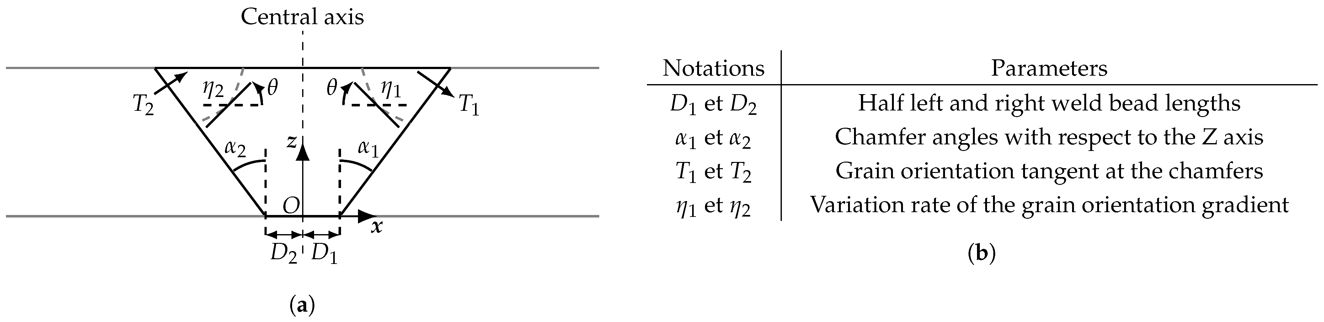
2.2. The Ogilvy’s Weld Description

In order to perform the ultrasonic imaging, one needs a weld description that preserves a realistic propagation of QL waves. In the optimization procedure, the Ogilvy’s weld model has been chosen for this task [20]. This description only requires a few parameters to provide an analytical law that defines the varying grain orientation. It is an instantaneous description of the weld and only adds four degrees of freedom to the optimization problem, when the model is applied in its simplest form for a symmetrical weld. This description is preferred over other approaches that would be more time consuming and add more parameters to the problem [15,16,21,22].
The grain orientation θ in the weld is defined by Ogilvy’s model as:
θ = arctan T 1 ( D 1 + z tan α 1 ) x η 1 with x > 0 arctan T 2 | D 2 + z tan α 2 | | x | η 2 with x < 0 π 2 with x = 0 .
The parameters to build this model are illustrated and summarized in Figure 1.
In the following numerical proof of concept, we use the simplest form of the Ogilvy’s model where D 1 = D 2 , α 1 = α 2 , T 1 = T 2 and η 1 = η 2 , and the weld crystalline structure is assumed to be orthotropic. The optimization procedure then involves 9 degrees of freedom: four Ogilvy’s model parameters, four components of the elastic tensor to account for the 2D QL waves propagation ( C 11 , C 13 , C 33 , C 55 ), and θ y the local disorientation of the polycrystalline structure with respect to θ in the imaging plan. This parameter indicates that the privileged dendritic growth during the weld cooling forms a θ y angle with the main direction of the polycrystalline structure.

2.3. The Particle Swarm Algorithm with Warm Restart

The optimization of the procedure is herein carried out by the particle swarm algorithm [23,24], used in the previous study [9], enhanced with a warm restart strategy [25]. Let us consider the swarm of particles represented by the position matrix X and randomly initialized in the weld parameters space. The displacement of the particles from the optimization step j to j + 1 is defined by
X j + 1 = X j + V j + 1 ,
where V j + 1 is the inertia of the particles at step j + 1 :
V j + 1 = α V j + β ( Q p X j ) + γ ( Q s X j ) .
Q p and Q s contain the best particle positions recorded by each individual particle on its path and by the whole swarm, respectively. The α , β and γ coefficients are chosen in order to penalize or not penalize the displacement of a particle with respect to V j , Q p and Q s . The initial velocity is set to V 0 = 0 .
The warm restart customization forces the particles to be randomly redistributed in the search space when the swarm has been stagnating in some sub-optimal area for a few iterations. It ensures that the algorithm extracts from critical points and reaches a better solution. The swarm however keeps track of the knowledge it has acquired on the solution space through the Q p and Q s parameters. In the following, for the numerical proof of concept and the two experimental cases, if the Q s value has not changed for 10 iterations, then the warm restarts is activated and it also reimburses the 10 iterations that have been lost during the stagnation.
We finally recall that the convergence of the swarm is driven by the standard deviations of each model parameter and by the standard deviation of the Amax value. The optimization stops when one of the supervised standard deviation reaches a selected threshold.

3. Numerical Application

In this section, we evaluate the optimization procedure on a numerical case with a symmetrical inhomogeneous and anisotropic weld. The inspection configuration is first described. The structure is designed so that the weld elasticity is coherent with a 316L stainless steel material and its dimensions are representative of the experimental applications hereafter. A sensitivity analysis based on the Sobol indices is then run in order to appraise the contribution of each parameter to the problem, before finally applying the optimization.

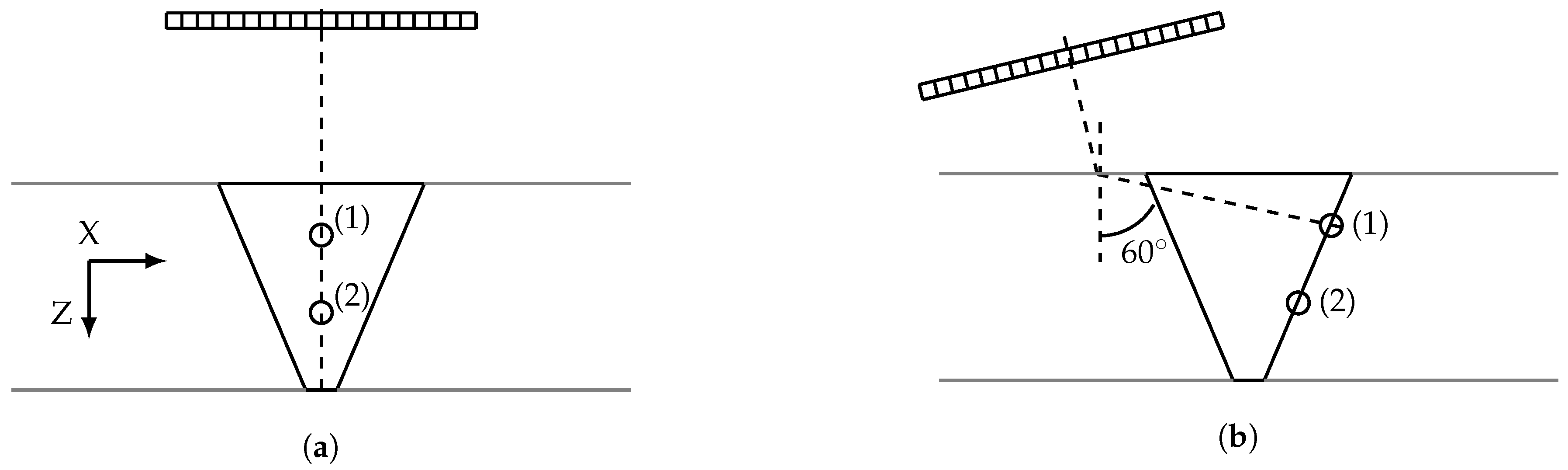
3.1. Configuration of Inspection

The weld is inspected with a normal incidence OL0°, where a probe is parallel to the flat and polished surface of the sample with a 20 mm water column height, as indicated in Figure 2. Two artificial Side-Drilled Holes (SDH) are vertically aligned in the middle of the weld at 10 mm (1) and 20 mm (2) depths and are of 1 mm diameter. The central axis of the array coincides with the alignment axis of the reflectors. The array operates around 5 MHz and is composed of 64 elements of 0.5 mm width with 0.6 mm pitch. Elements are excited with a Gaussian-type pulse with 80% bandwidth at 6 dB and sampled at 100 MHz.
The actual values of the 9 weld model parameters to be varied are indicated in Table 1. The base material is made of isotropic 316L stainless steel where longitudinal waves propagate with a phase velocity of 5720 m·s−1. Echoes are simulated in CIVA using the method of separation of variables [26], without accounting for attenuation.
The TFM images are computed in a 10 × 10 mm2 region composed 51 × 101 pixels around defect (1). The resolution in the imaging zone is approximatively λ / 5 along the X axis and λ / 10 along the Z axis, where λ = 1.14 mm is the wavelength of a longitudinal wave emitted at 5 MHz and travelling at 5720 m·s−1.

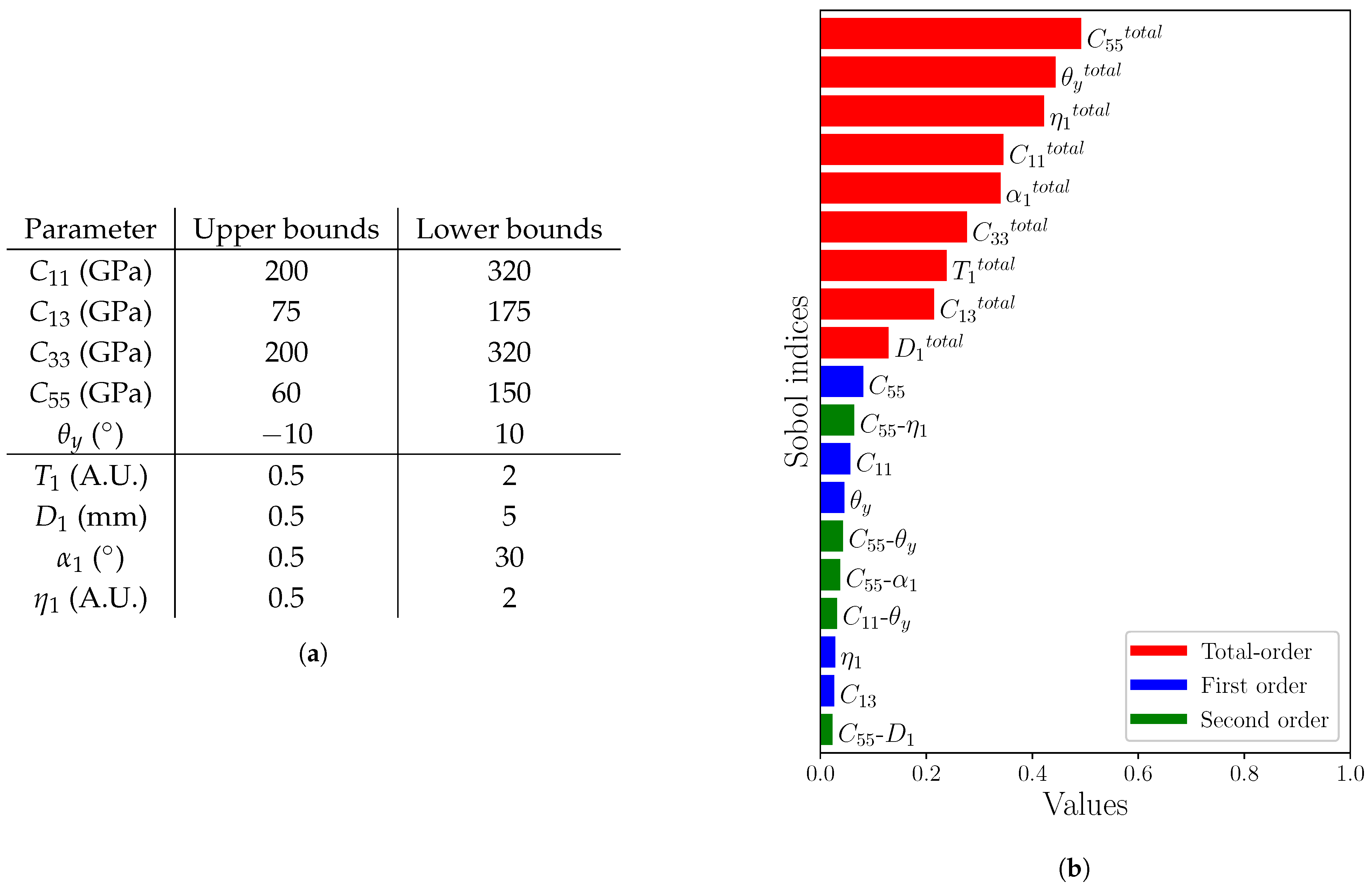
3.2. Sobol Sensitivity Analysis

Before applying the optimization procedure, a Sobol analysis is conducted, as it was done in [9]. The aim of this analysis is to explain the contribution of each parameter to the Amax variations. Three Sobol indices are derived from 5 × 10 5 images: the first-order index which indicates the contribution of a sole varying parameter; the second-order index for the combined contribution of two parameters; and the total index that represents the contribution of a parameter while taking into account all the interactions it has with the others. The range of variation of each parameter and the sensitivity results are displayed in Figure 3. For readability, only indices of value greater than 5 × 10 2 are displayed.
Every parameter appears to have a non negligible contribution to the variation of Amax, as shown by the total-order indices. None of these parameters can then be discarded from the optimization problem. The total contribution of each parameter seems not to be driven by its individual variations but by its cross-variations with the other parameters, as it is highlighted by the small values of first-order indices. Moreover, the sum of the total-order indices is not equal to one, which suggests that the parameters are correlated with one another.
It should be pointed out that these results are case-dependent and can be very different with another application (other materials, defects, probes, etc.). That the total index of some parameters is higher than others is directly related to this specific inspection case. For example, D 1 contributes less than C 55 simply because the inspected defect is localized at the centre of the weld, where the bead length has little influence.

3.3. Application of the Optimization

The procedure is now applied with the simulated signals. The hyper-parameters of PSO are set so α = β = γ = 0.5 , with a swarm composed of 40 particles and a maximum of 3 warm restarts. The initial maximum number of iterations is 30, which can go up to 60 if the 3 warm restarts are activated (+10 iterations by restart). The bounds of the exploration space are the same as for the sensitivity analysis in Figure 3. The supervised convergence thresholds of the model parameters are indicated in Table 2. The threshold on the Amax criterion is 10 3 , as the Amax values are of a unitary order of magnitude. They are set to correspond to a small estimation error on the material properties and on the Amax value.
The procedure is statistically evaluated with 100 optimization trials from which we derive several metrics: convergence rate; number of iterations before convergence; error on the echo localization for defect (1); error on the material properties estimation. The convergence rate is defined by the number of optimized images for which Amax ≥ Aref − 2 dB, where Aref is the maximum amplitude in the image computed with the actual material properties. The values of the different metrics are presented in Table 3.
In terms of imaging, the procedure shows very good performances with a success rate of 98%. The estimation of the position of defect (1) is also very good with errors inferior to 1 mm along each direction in the image.
The time needed to reach convergence is satisfactory with approximately 21 iterations, which corresponds to the computation of 840 images for one optimization trial. The computations were performed with an 8-core Intel® Xeon® E3-1240 v6 at 3.70 GHz, with which a TFM image of 51 × 101 pixels is computed in 0.83 s. Thus, the 840 images are computed in less than 12 min.
However, the estimation of the unknown properties of the weld fails to provide accurate values. This is due to a strong diversity of solutions that is directly related to the use of a single scalar (Amax) to determine the quality of a TFM image. The parameter estimation is then only reliable around the inspected defect, and with 9 unknown correlated parameters with a more or less major contribution, this leads to a great variety of results. As was mentioned in the sensitivity analysis, the position of the reflector at the center of the weld also penalizes the estimation of the less contributing parameters like D 1 which is representative of the weld width.
Despite the procedure not being able to accurately estimate the weld properties, it remains reliable for imaging as exemplified in Figure 4 where three images are displayed: computed with an isotropic weld model (a); with the actual material properties (b); and an optimized one (c). The optimized image was randomly chosen from the 100 solutions of the optimization trials and is a good representation of the other optimized images. For each image, side-plots contain the horizontal and vertical echodynamic curves (i.e., evolution of the maximum amplitude along each axis).
In the optimized image, the degradations due to a wrong reconstruction model are corrected and the defects are now clearly identifiable. Furthermore, the optimized image and the one computed with the actual material properties look very similar. Compared to the degraded image computed with the isotropic reconstruction model (a), the Amax value is increased by 17 dB in the optimized image (c). This amplitude is comparable to the reference image computed with the actual material properties (b) for which the gain is also +17 dB. The correlation coefficient between the reference and optimized images is 0.97 , which confirms that the images are almost identical. The material properties used to compute the optimized image are indicated in Figure 5 along with the estimation errors. The actual and estimated slowness curves and the estimation error are also displayed.
The slowness estimation error is inferior to 5.0 %, with a mean error of 13.4 % on the elastic properties. The mean error on the Ogilvy’s parameters is 32.1 %.
Thereby, the proposed optimization procedure applied to this proof of concept shows promise for improving the quality of TFM images in nuclear welds with experimental data, even though it estimates the material properties with poor accuracy.

4. Experimental Applications

This last section is dedicated to the experimental application of the optimization procedure. Two V-shape weld samples provided by Electricité De France (EDF) are considered. They come from the same weld but they contain artificial defects at different locations. Therefore, a cross-comparison of the optimization results can be carried out.

4.1. Configurations of Inspection

Hereafter, two samples lent by EDF and extracted from the same weld are inspected. Each of them comprises two SDH of 1 mm diameter at different positions: in the first sample the defects are located at the same positions as in the numerical proof of concept; in the second sample the reflectors are on the right chamfer at 10 mm and 20 mm depths. Consequently, the first sample is inspected with a OL0° inspection and the second one with a OL60° inspection (the probe is tilted in the water so that the QL wave propagation in the base material is refracted with a 60o angle). The configurations of inspection are illustrated in Figure 6. A macrograph of the weld and two photographs of the samples are given in Figure 7. The two samples have the same height.
The data acquisitions were performed with a multichannel MultiX++TM (Eddyfi Technologies, Québec, QC, Canada) and a 5 MHz linear array (Imasonic, Voray-sur-l’Ognon, France) composed of 64 elements of 0.5 mm width and with a 0.6 mm pitch. The array elements were excited with a rectangular-type electric pulse whose time length is 0.2 μs, and signals were digitized with a sampling frequency of 100 MHz.

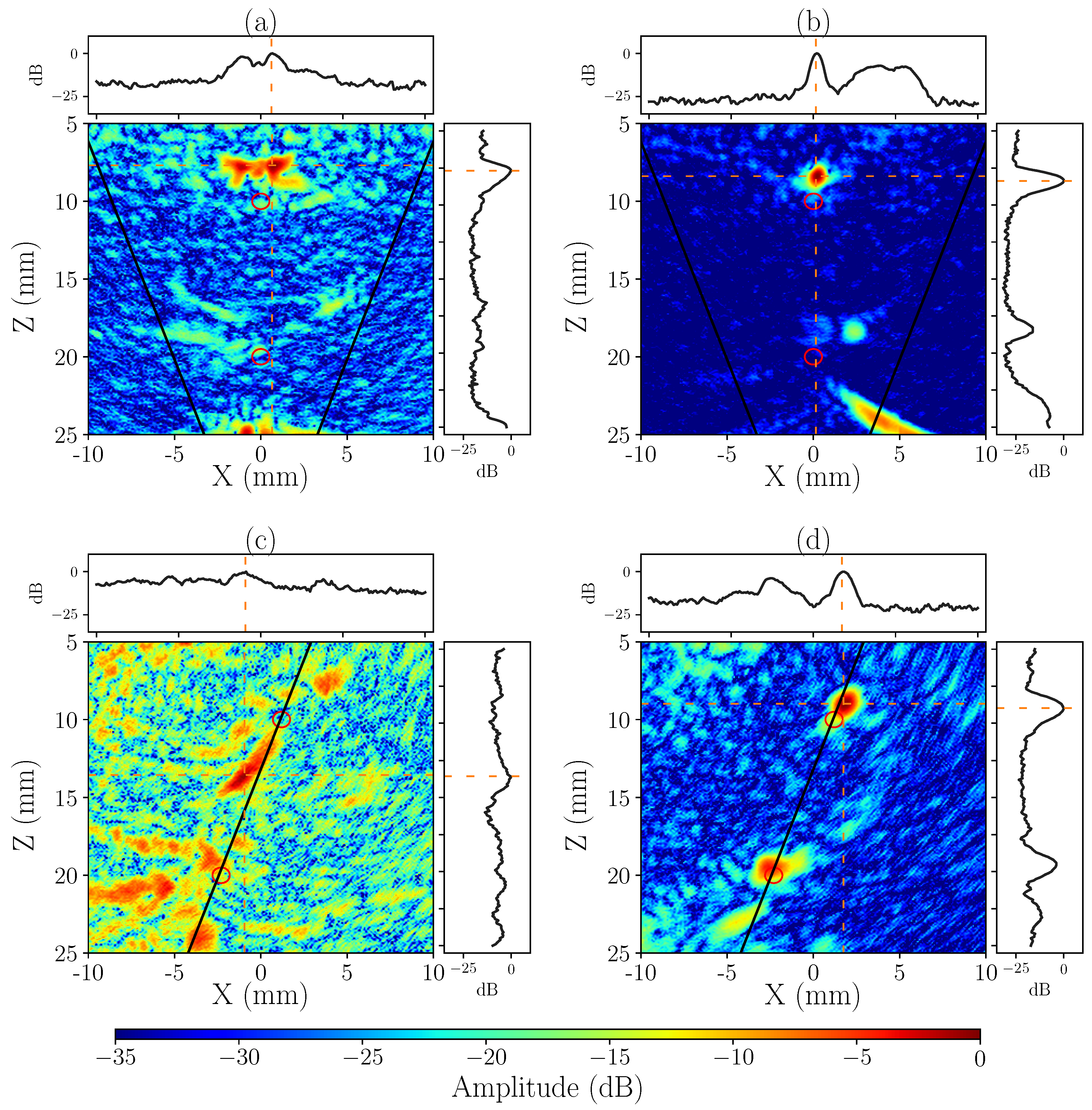
4.2. Application of the Optimization

We have little information on the material properties, especially concerning its elasticity. It is therefore a blind-test application of the procedure. The base material is 316L stainless steel where the celerity of longitudinal waves is 5720 m·s−1 and we set the density to ρ = 7.80 g·cm−3.
As we can see on the macrograph and photographs, the dendritic structure of the weld is asymmetrical and shows a tilt of about 20 ° of the main axis of the grains. Thus, to account for this dissymmetry, the eight Ogilvys’ parameters should all be used ( D 1 D 2 , α 1 α 2 , T 1 T 2 and η 1 η 2 ). We also discard the θ y parameter and we introduce a new parameter ζ , which is the disorientation angle of the main axis of the grains with respect to the Z axis. The optimization is now conducted on 13 parameters instead of 9.
Again, the optimization is evaluated over 100 trials for each case with the same hyper-parameter values as in the numerical application. The imaging area is restricted around defect (1) during the optimization and has the same size and definition as before. The performance metrics are summarized in Table 4 for the two configurations of inspection. As we do not precisely know the material properties, the estimation error of the weld properties is replaced by the dispersion of the results, with respect to the mean values of the parameters within the upper and lower bounds defined for the exploration space.
These experimental results are in good agreement with the numerical case. For both weld samples, the convergence rate is once again satisfactory with weak errors on the positioning of the defect echo. We can however remark that the numbers of iterations before satisfying the convergence criteria are different and that the procedure converges faster with an OL60° configuration than with an OL0° configuration.
Here again, the dispersion of the weld models after the optimization is non-negligible in both cases, although they are found to be better than in the previous simulated application. The characterization of the material is consequently not accurately achieved because of the non-uniqueness of the solution due to many varying unknown parameters.
To exemplify the improvement of the images after the optimization, two final images are randomly picked from the 100 trials of the two inspection cases and are displayed in Figure 8. They are accompanied by the corresponding degraded images, due to the use of the isotropic reconstruction model. The weld model parameters used to compute the optimized images are indicated in Figure 9 along with the associated slowness curves.
The final images show a great improvement of their quality and we measure a +10 dB Amax increase in both cases. The degradation of the echo of the defect (1) is each time corrected and the positioning errors of this defect are inferior to 1 mm. We also notice that the echo of defect (2) is well corrected for the OL60° configuration, with a good estimation of position. However, in the OL0° configuration, the second echo is hardly invisible and seems misplaced. This is directly caused by the first reflector that hides the second one.
As one can see, the material properties and slowness curves used to compute these two images are very different but they produce much higher quality TFM images. Therefore, though the dispersion of the results is very large, one may wonder if there exist common weld models between the two cases.

4.3. Cross-Comparison of the Estimated Weld Models

Thanks to the two mock-ups being sampled from a same weld, we can perform a cross-comparison of the results. In a first step, the 100 weld models obtained with the OL0° inspection are compared with the 100 weld models resulting from the OL60° inspection in order to find a common model. The second step consists in applying the reconstruction models obtained for the 100 trials in the OL0° case to the signals recorded with the OL60° case, and vice-versa.
In order to determine common models, a tolerance error is defined that indicates the minimum admissible difference for models to be similar. This criterion is set to 10 GPa for the elastic components, 0.5 mm for D 1 , 2 , 3 ° for both α 1 , 2 and ζ , and 0.25 A.U. for both T 1 , 2 and η 1 , 2 . However, after comparison, none of the models satisfies the fixed tolerance error, which means that no model is common to the results of the 100 optimization trials in the OL0° case and to the 100 trials in the OL60° case. The dispersion of the results is here again too large to find a common model.
Let us consider now the 100 weld models obtained from the OL0° inspection and apply them to the set of signals recorded with the OL60° configuration. It turns out that none of the models produces a satisfactory image. On the contrary, the images are as degraded as with an isotropic reconstruction model. An example is presented in Figure 10b. Nonetheless, if we consider the 100 weld models resulting from the OL60° inspection and apply them to images computed with the OL0° acquisition, we find that one model is able to correct the image with the OL0° configuration. This image is displayed in Figure 10a and the associated weld model parameters are indicated in Table 5. It would be interesting to compare these values with those resulting from another experimental characterization setup to see how realistic or unrealistic these results are.
This experimental application of the optimization procedure confirms the results of the numerical study: the optimization is very efficient in correcting the degradation of TFM images and produces high quality images, but the weld model parameters cannot be accurately estimated as the optimization only relies on the observation of a single isolated defect. In this section, two samples extracted from the same weld were considered, however the dispersion of the estimated weld parameters is too strong to find a common model between both cases. At the end, only one model is able to both correct the images of the inside of the two samples.

5. Conclusions

In this study, we investigated the ability of an optimization procedure to enhance the quality of TFM images of point-like reflectors inside unknown anisotropic and inhomogeneous nuclear welds. The procedure was first evaluated with simulated data and it was shown that it was able to correct the degradation of the image due to the unknown material properties, with good performance. The defect echoes were accurately estimated with less than 1 mm errors, although it was also observed that the estimation of the material properties could not be precisely achieved. The dispersion of the results with a value of 26%, which was a consequence of the optimization only being realized around a single isolated defect, was way too strong to provide a fair characterization of the whole structure. The properties estimation was then only reliable in the region around the reflector. Moreover, a sensitivity analysis demonstrated that the several unknown parameters of the weld model were correlated with one another and that their respective contributions were mainly driven by their mutual interactions rather than by their single effect. Therefore, a great variety of combinations was solution to the optimization problem.
An experimental application of the procedure with two samples from a same weld confirmed the results of the numerical proof of concept. The reflectors were hardly visible on the images computed with an isotropic reconstruction model, but after the optimization, the two defects were clearly visible and their localization was well estimated. Here again, the final images were of very satisfactory quality with positioning errors inferior to 1 mm, but the material estimation was not accurate due to the substantial dispersion, which was upwards of 15%. A cross-comparison of the material properties after optimization indicated that there was no common weld model between the two experimental cases. It was however found that one model taken from one result on the second sample was able to correct the image in both cases. Nevertheless, our aim was to implement an optimization procedure to correct the images and, as such, the proposed approach emphatically succeeds at this task.
Several methods of improvement are considered for future works. The main challenge is to reduce the computation times needed for the optimization. This should be achieved by further tuning the hyper-parameters of the particle swarm algorithm to reduce the number of iterations needed to reach an optimal result, and by using the CUDA architecture to parallelize the computations in order to shorten the time needed by CIVA to compute the images. Some interest has also to be taken in the a priori information that we can use to reduce the exploration space range and thus to reduce the dispersion of the results. Finally, the optimization procedure should be evaluated for crack-type defects that are of real concern in the NDT domain.

Author Contributions

Conceptualization, C.M., S.R. and D.L.; methodology, C.M., S.R.; software, C.M.; validation, C.M. and S.R.; formal analysis, C.M.; investigation, C.M.; data curation, C.M.; writing—original draft preparation, C.M.; writing—review and editing, C.M., S.R. and D.L.; visualization, C.M.; supervision, S.R. and D.L.; project administration, S.R. and D.L.; funding acquisition, S.R. All authors have read and agreed to the published version of the manuscript.

Funding

This study is part of European project ADVISE, that has received funding from the Euratom research and training programme 2014–2018 under grant agreement No. 755500.

Acknowledgments

The authors would like to thank the ADVISE project partners, with special credits to Electricité De France (EDF) for providing mock-ups to all consortium partners.

Conflicts of Interest

The authors declare no conflict of interest.

References

  1. Drinkwater, B.W.; Wilcox, P.D. Ultrasonic arrays for non-destructive evaluation: A review. NDT E Int. 2006, 39, 525–541. [Google Scholar] [CrossRef]
  2. Holmes, C.; Drinkwater, B.W.; Wilcox, P.W. The post-processing of ultrasonic array data using the total focusing method. Insight 2004, 46, 677–680. [Google Scholar] [CrossRef]
  3. Prada, C.; Fink, M. Eigenmodes of the time reversal operator: A solution to selective focusing in multiple-target media. Wave Motion 1994, 20, 151–163. [Google Scholar] [CrossRef]
  4. Fink, M.; Cassereau, D.; Derode, A.; Prada, C.; Roux, P.; Tanter, M.; Thomas, J.L.; Wu, F. Time-reversed acoustics. Rep. Prog. Phys. 2000, 63, 1933–1995. [Google Scholar] [CrossRef]
  5. Le Jeune, L.; Robert, S.; Dumas, P.; Membre, A.; Prada, C. Adaptive ultrasonic imaging with the total focusing method for inspection of complex components immersed in water. In Proceedings of the 41st Annual Review of Progress in Quantitative Nondestructive Evaluation, Boise, ID, USA, 20–25 July 2014; Volume 1650, pp. 1037–1046. [Google Scholar]
  6. Hoyle, E.; Sutcliffe, M.; Charlton, P.; Rees, J. Virtual source aperture imaging with auto-focusing of unknown complex geometry through dual layered media. NDT E Int. 2018, 98, 55–62. [Google Scholar] [CrossRef]
  7. David, S.A.; Vitek, J.M. Correlation between solidification parameters and weld microstructures. JOM 2003, 55, 14–20. [Google Scholar] [CrossRef]
  8. David, S.A.; Babu, S.S.; Vitek, J.M. Welding: Solidification and microstructure. Int. Mater. Rev. 1989, 34, 213–245. [Google Scholar] [CrossRef]
  9. Menard, C.; Robert, S.; Miorelli, R.; Lesselier, D. Optimization algorithms for ultrasonic array imaging in homogeneous anisotropic steel components with unknown properties. NDT E Int. 2020, 116, 102327. [Google Scholar] [CrossRef]
  10. Gengembre, N.; Lhémery, A. Pencil method in elastodynamics: Application to ultrasonic field computation. Ultrasonics 2000, 38, 495–499. [Google Scholar] [CrossRef]
  11. Gardahaut, A.; Jezzine, K.; Cassereau, D. Paraxial Ray-Tracing Approach for the Simulation of Ultrasonic Inspection of Welds; American Institute of Physics: College Park, MD, USA, 2014; Volume 1581, pp. 529–536. [Google Scholar]
  12. Pudovikov, S.; Bulavinov, A.; Pinchuk, R. Innovative Ultrasonic Testing (UT) of nuclear components by sampling phased array with 3D visualization of inspection results. In Proceedings of the JRC-NDE 2010 8th International Conference on NDE in Relation to Structural Integrity for Nuclear and Pressurized Components, Berlin, Germany, 29 October–1 November 2010; pp. 910–917. [Google Scholar]
  13. Juengert, A.; Dugan, S.; Homann, T.; Mitzscherling, S.; Prager, J.; Pudovikov, S.; Schwender, T. Advanced ultrasonic techniques for Nondestructive Testing of austenitic and dissimilar welds in nuclear facilities. In Proceedings of the 44th Annual Review of Progress in Quantitative Nondestructive Evaluation, Provo, UT, USA, 16–21 July 2017; Volume 1949, p. 110002. [Google Scholar]
  14. Chassignole, B.; Recolin, P.; Leymarie, N.; Gueudré, C.; Guy, P.; Elbaz, D. Study of ultrasonic characterization and propagation in austenitic welds: The MOSAICS project. In Proceedings of the 41st Annual Review of Progress in Quantitative Nondestructive Evaluation, Boise, ID, USA, 20–25 July 2014; Volume 1650, pp. 1486–1495. [Google Scholar]
  15. Tant, K.M.M.; Galetti, E.; Curtis, A.; Mulholland, A.J.; Gachagan, A. A transdimensional Bayesian approach to ultrasonic travel-time tomography for nondestructive testing. Inverse Probl. 2018, 34, 095002. [Google Scholar] [CrossRef] [Green Version]
  16. Fan, Z.; Mark, A.F.; Lowe, M.J.S.; Withers, P.J. Nonintrusive estimation of anisotropic stiffness maps of heterogeneous steel welds for the improvement of ultrasonic array inspection. IEEE Trans. Ultrason. Ferroelectr. Freq. Control 2015, 62, 1530–1543. [Google Scholar] [CrossRef] [PubMed] [Green Version]
  17. Zhang, J.; Hunter, A.J.; Drinkwater, B.W.; Wilcox, P.D. Monte Carlo inversion of ultrasonic array data to map anisotropic weld properties. IEEE Trans. Ultrason. Ferroelectr. Freq. Control 2012, 59, 2487–2497. [Google Scholar] [CrossRef]
  18. Stojakovic, D. Electron backscatter diffraction in materials characterization. Process. Appl. Ceram. 2012, 6, 1–13. [Google Scholar] [CrossRef]
  19. Mark, A.F.; Li, W.; Sharples, S.; Withers, P.J. Comparison of grain to grain orientation and stiffness mapping by spatially resolved acoustic spectroscopy and EBSD. J. Microsc. 2017, 267, 89–97. [Google Scholar] [CrossRef] [PubMed] [Green Version]
  20. Ogilvy, J.A. Computerized ultrasonic ray tracing in austenitic steel. NDT E Int. 1985, 18, 67–77. [Google Scholar] [CrossRef]
  21. Gueudré, C.; Le Marrec, L.; Moysan, J.; Chassignole, B. Direct model optimization for data inversion. Application to ultrasonic characterization of welds. NDT E Int. 2009, 42, 47–55. [Google Scholar] [CrossRef]
  22. Tant, K.M.M.; Galetti, E.; Mulholland, A.J.; Curtis, A.; Gachagan, A. Effective grain orientation mapping of complex and locally anisotropic media for improved imaging in ultrasonic non-linear testing. Inverse Probl. Sci. Eng. 2020, 28, 1694–1718. [Google Scholar] [CrossRef]
  23. Kennedy, J.; Eberhart, R. Particle swarm optimization. In Proceedings of the International Conference on Neural Networks, Perth, Australia, 27 November–1 December 1995; Volume 4, pp. 1942–1948. [Google Scholar]
  24. Trelea, I.C. The particle swarm optimization algorithm: Convergence analysis and parameter selection. Inf. Process. Lett. 2003, 85, 317–325. [Google Scholar] [CrossRef]
  25. García-Nieto, J.; Alba, E. Restart particle swarm optimization with velocity modulation: A scalability test. Soft Comput. 2011, 15, 2221–2232. [Google Scholar] [CrossRef]
  26. Darmon, M.; Leymarie, N.; Chatillon, S.; Mahaut, S. Modelling of scattering of ultrasounds by flaws for NDT. In Ultrasonic Wave Propagation in Non Homogeneous Media; Springer: Berlin/Heidelberg, Germany, 2009; pp. 61–71. [Google Scholar]
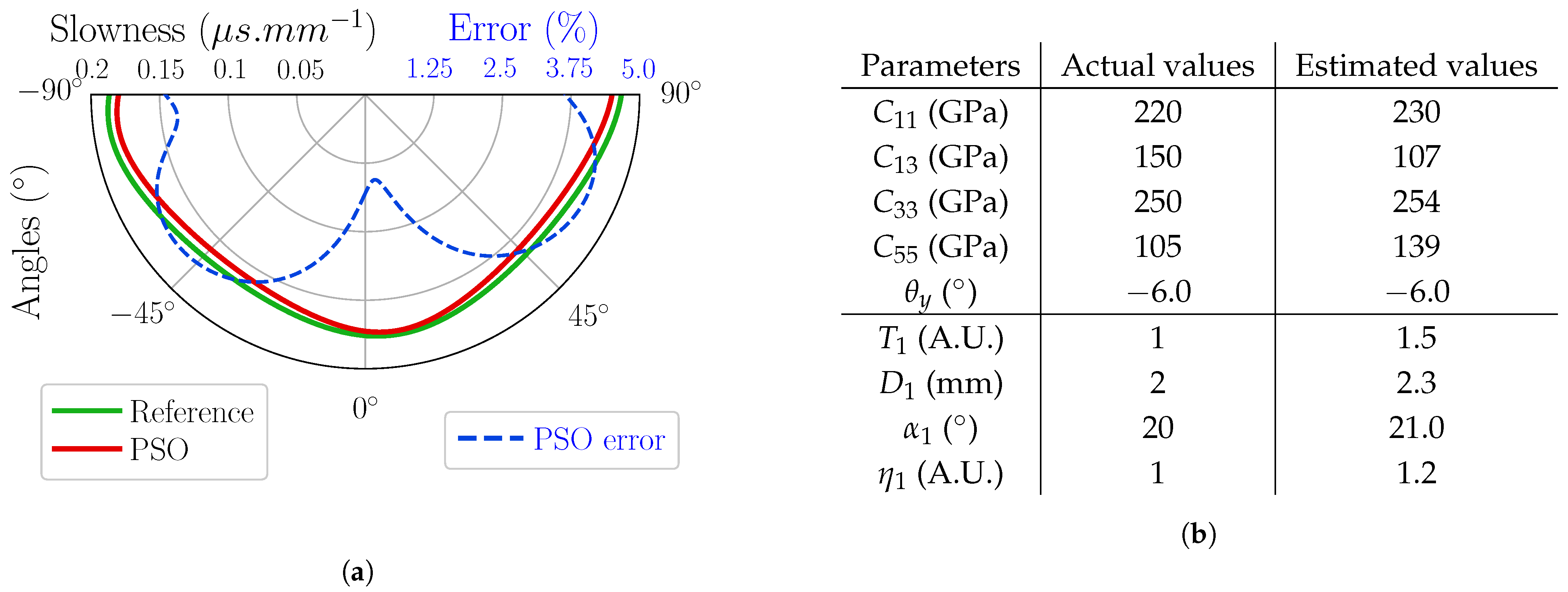
Figure 1. Ogilvy’s model: (a) geometrical description of the model and (b) specific parameters. T 2 , D 1 and α 1 are positive values while T 1 , D 2 and α 2 are negative values. η 1 et η 2 always are positive.
Applsci 11 06505 g001
Figure 2. Scheme of the numerical setup: immersion inspection using an array placed 20 mm above the surface; 316L stainless steel-based V-shape weld with two Side-Drilled Holes (SDH) of 1 mm diameter vertically aligned in the middle of the structure at depths 10 mm (1) and 20 mm (2) from the surface.
Applsci 11 06505 g002
Figure 3. Upper and lower bounds of the variation range of each parameter (a). Sobol indices of first, second and total-order (b). Only indices of values larger than 5 × 10 2 are shown.
Applsci 11 06505 g003
Figure 4. Images in a 316L stainless steel V-shape weld with simulated signals: isotropic reconstruction model (a); actual material properties (b); PSO optimization (c). The vertical and horizontal echodynamic curves are presented in the side-plots. The optimization is conducted around SDH (1), and each image is normalized by the maximum amplitude in a 10 × 10 mm2 region around this defect (the amplitude of this defect echo is 0 dB for all images). Orange dashed lines indicate the Amax position around defect (1) and black lines indicate the chamfers of the weld.
Applsci 11 06505 g004
Figure 5. Slowness curves of QL waves and estimation error of the optimization procedure (a): actual material properties (green) and estimation by the optimization procedure (red); estimation error of slowness with PSO (dashed blue). Table of actual and estimated material properties (b).
Applsci 11 06505 g005
Figure 6. Configurations of inspection of the two 316L stainless steel V-shape weld samples: OL0° inspection (a) and OL60° inspection (b). Each sample contains two 1.0 mm diameter SDH at 10 mm (1) and 20 mm (2) depths. The reflectors of the first sample are vertically aligned in the middle of the weld and those of the second sample are located on the right chamfer.
Applsci 11 06505 g006
Figure 7. Macrograph of the weld lent by EDF (a). Photographs of the two samples (b) et (c). The two samples have the same height.
Applsci 11 06505 g007
Figure 8. Images in a 316L stainless steel V-shape weld with experimental signals: isotropic reconstruction model (a,c); PSO optimization (b,d). The vertical and horizontal echodynamic curves are presented in the side-plots. The optimizations are conducted around SDH (1), and each image is normalized by the maximum amplitude in a 10 × 10 mm2 region around this defect (the amplitude of this defect echo is 0 dB for all images). Orange dashed lines indicate the Amax position around defect (1) and black lines indicate the chamfers of the weld.
Applsci 11 06505 g008
Figure 9. Slowness curves of QL waves estimated with PSO (a): slowness curves for the OL0° inspection (red), the OL60° inspection (purple) and the base material (orange). Table of the material properties values after optimization (b).
Applsci 11 06505 g009
Figure 10. Images in a 316L stainless steel V-shape weld with experimental signals: images computed from the acquisition with the OL0° experimental setup and by using a weld model provided by the optimization of the image for the OL60° configuration (a); image from the OL60° configuration computed with a weld model resulting from the optimization of the image for the OL0° configuration (b).
Applsci 11 06505 g010
Table 1. Actual values of the 9 unknown parameters of the weld.
ElasticityValuesOgilvy’s ModelValues
C 11 220 GPa T 1 = T 2 1 A.U.
C 13 150 GPa D 1 = D 2 2 mm
C 33 250 GPa α 1 = α 2 20 °
C 55 105 GPa η 1 = η 2 1 A.U.
θ y 6 °
Table 2. Supervised convergence thresholds for the weld model parameters.
ElasticityThresholdOgilvy’s ModelThreshold
C 11 5 GPa T 1 = T 2 0.05 A.U.
C 13 5 GPa D 1 = D 2 0.1 mm
C 33 5 GPa α 1 = α 2 0.2 °
C 55 5 GPa η 1 = η 2 0.05 A.U.
θ y 0.3 °
Table 3. Performances of the optimization procedure with simulated data: values obtained with 100 optimization trials.
MetricsValues
Convergence rate98%
Number of iterations 20.9 ± 9.4
Weld model estimation error 20.8 ± 26.0 %
Error X 0.1 ± 0.1 mm
Error Z 0.5 ± 0.3 mm
Table 4. Performances of the optimization procedure with experimental data obtained with OL0° and OL60° configurations of inspection on two samples of the same weld: values obtained with 100 optimization trials.
MetricsOL0°OL60°
Convergence rate (%)8486
Number or iterations 30.3 ± 18.6 12.1 ± 8.4
Weld model dispersion (%) 17.5 18.2
Error X (mm) 0.7 ± 0.4 1.0 ± 0.6
Error Z (mm) 0.3 ± 0.2 0.3 ± 0.2
Table 5. Weld model parameter values obtained from the optimization with the OL60° configuration and applied to compute the OL0° image in Figure 10.
ParametersOL60° Estimated Values
C 11 (GPa)229
C 13 (GPa)137
C 33 (GPa)257
C 55 (GPa)129
T 1 (A.U.) 1.1
T 2 (A.U.) 1.0
D 1 (mm) 3.7
D 2 (mm) 0.6
α 1 ( ° ) 32.1
α 2 ( ° ) 5.0
η 1 (A.U.) 0.8
η 2 (A.U.) 1.1
ζ ( ° ) 28.5
Publisher’s Note: MDPI stays neutral with regard to jurisdictional claims in published maps and institutional affiliations.

