
Lp-Norm Inversion of Gravity Data Using Adaptive Differential Evolution


Abstract
:1. Introduction
2. Differential Evolution
2.1. Standard Differential Evolution Algorithm
- (1)
- Initialization
- (2)
- Mutation
- (3)
- Crossover
- (4)
- Selection
2.2. Improved Differential Evolution Algorithm
- (1)
- Improvement of Mutation Strategy
- (2)
- Adaptive Guided Evolution
2.3. Control Parameters Adaptation of DE Algorithm
3. Lp-Norm Gravity Inversion Based on Adaptive Differential Evolution
3.1. Forward Modeling
3.2. Inversion Method
3.3. Adaptive Adjustment of Regularization Factor
3.4. Implement of Inversion Algorithm
| Algorithm 1. Lp-norm inversion of gravity based on an improved adaptive differential evolution. |
| 1: = 1 2: Set = 100, = 0.5, = 0.5, = 0.5, = 0.1, = 0.05, initialize population , initialize the regularity coefficient , evaluation the population . 3: While termination conditions are not met do 4: 5: For to do 6: ; 7: ; 8: 9: End For 10: For do 11: Generate mutation vector according to mutation strategy (12) 12: Generate trial vector from (8) 13: End For 14: Evaluation test vector 15: Form a new population according to Equation (9) 16: Update and according to Equations (16)–(18), update according to (14), update by (27). 17. End While |
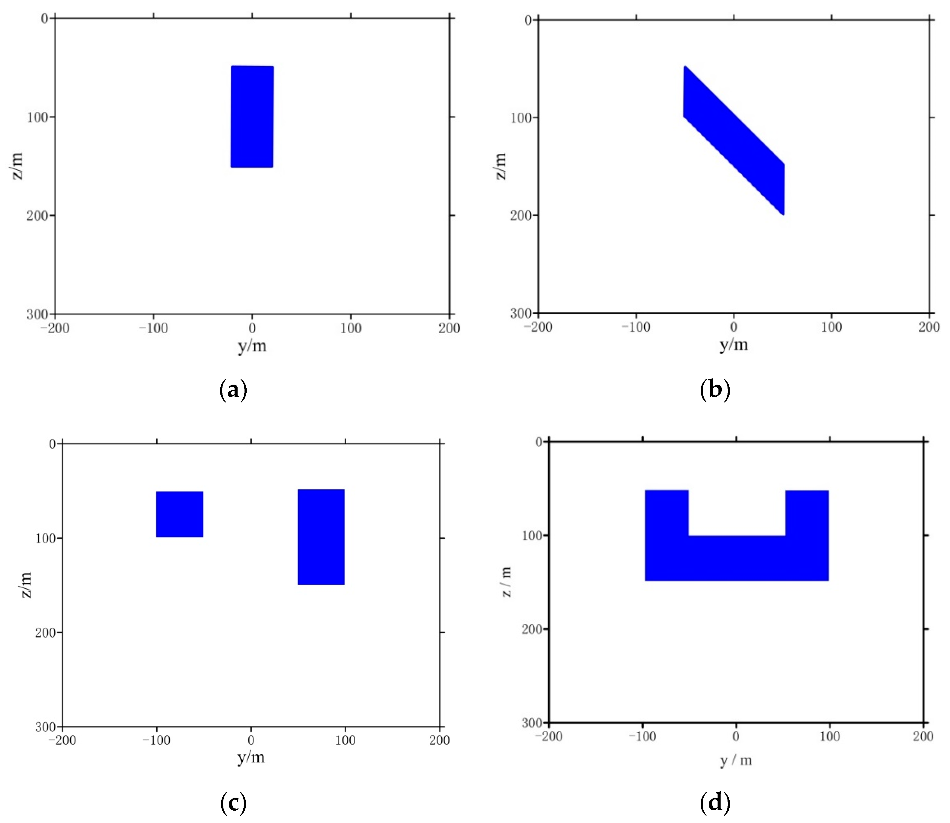
4. Simulation Tests
4.1. Parameter Setting
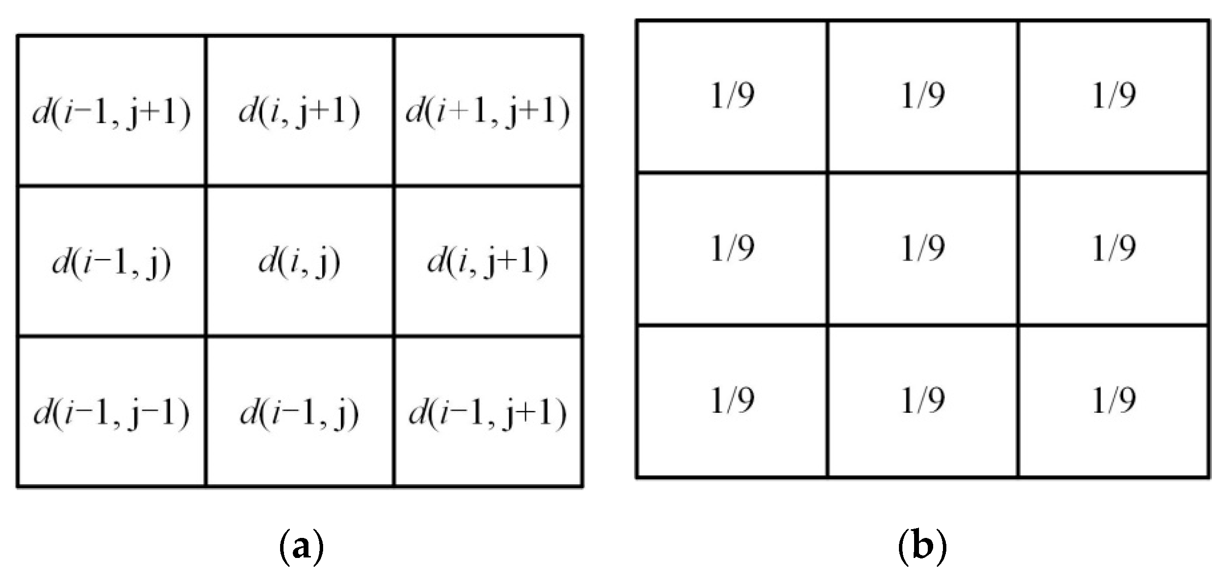
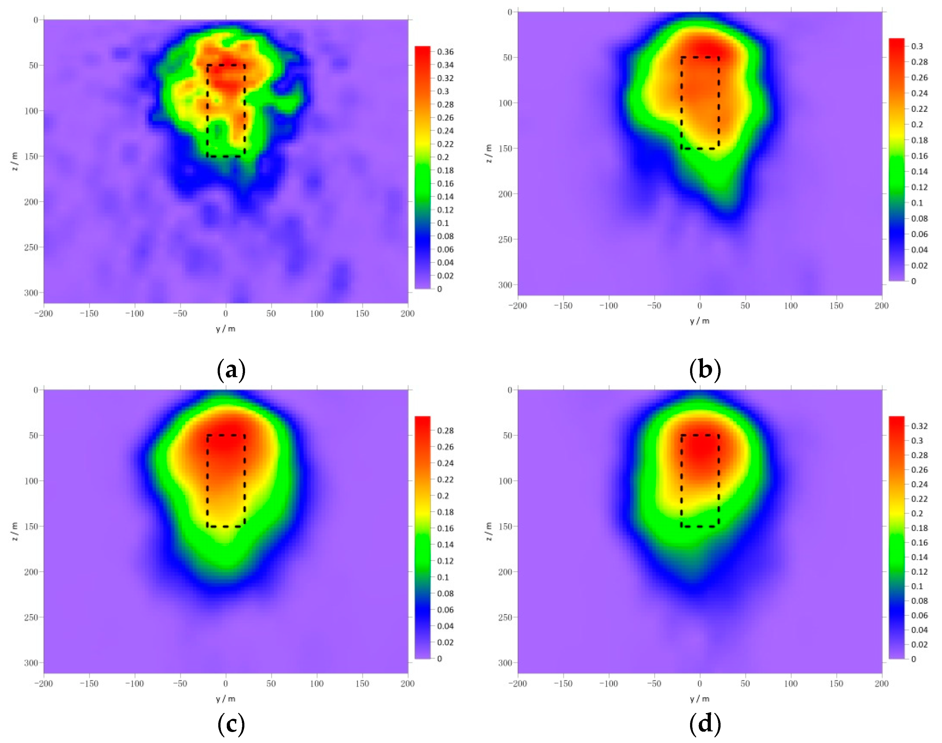
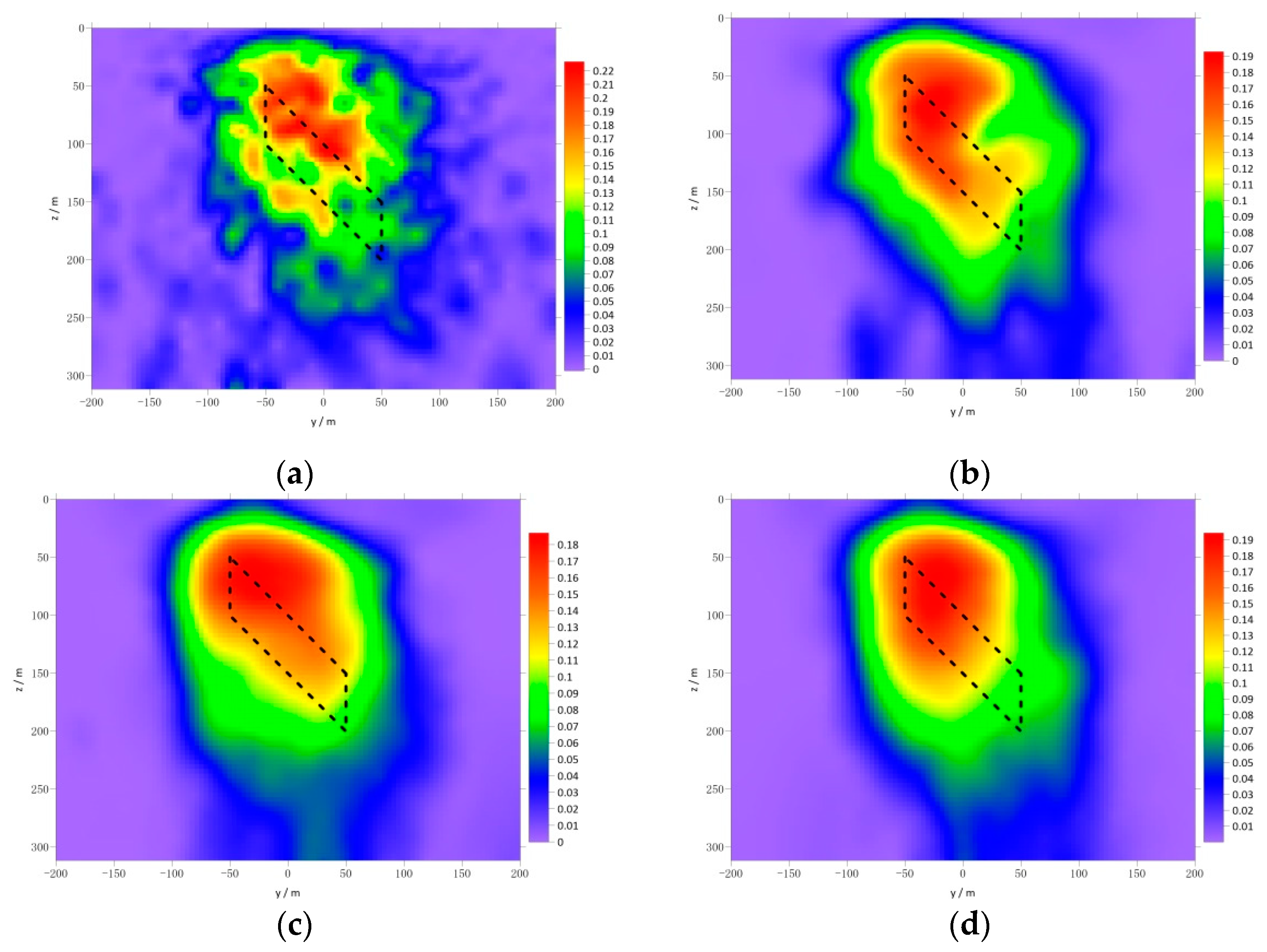
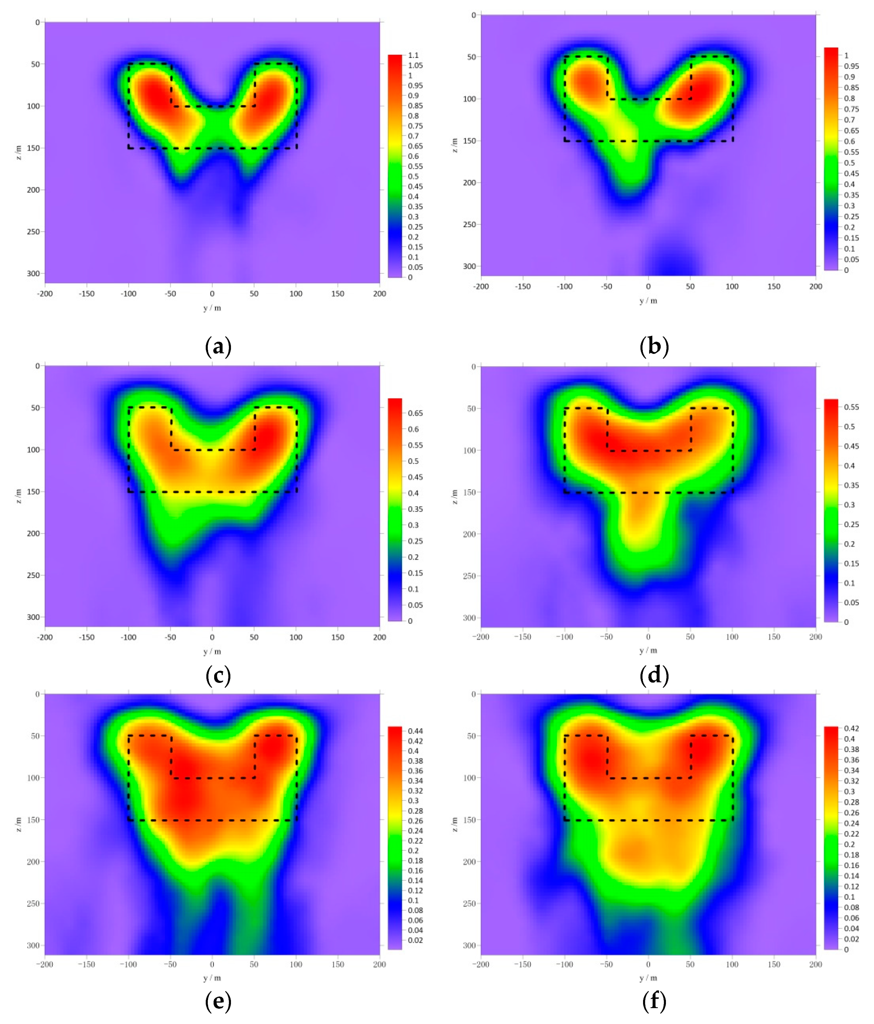
4.2. The Impact of Weighted Moving Average Smoothing
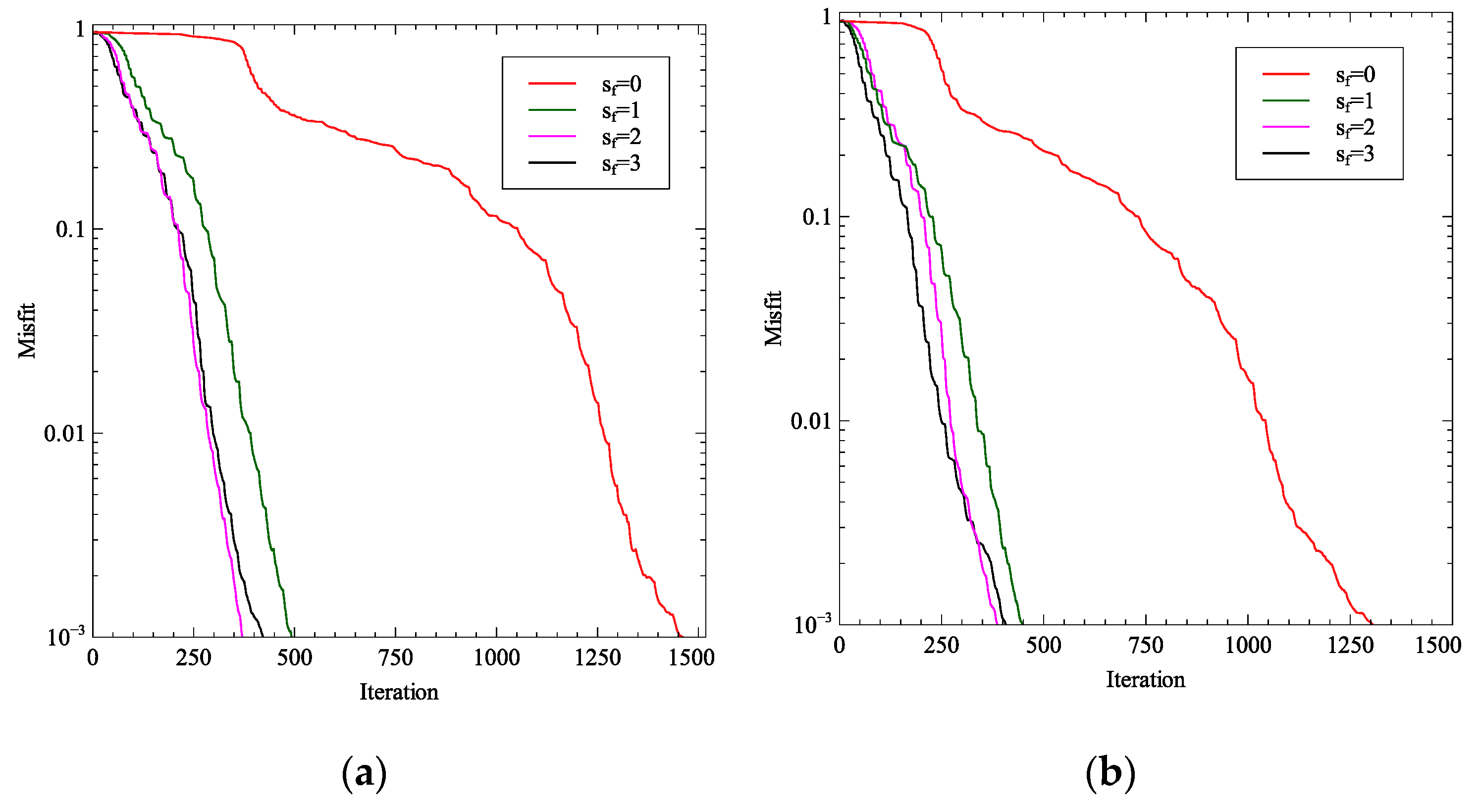
4.3. The Effect of Value
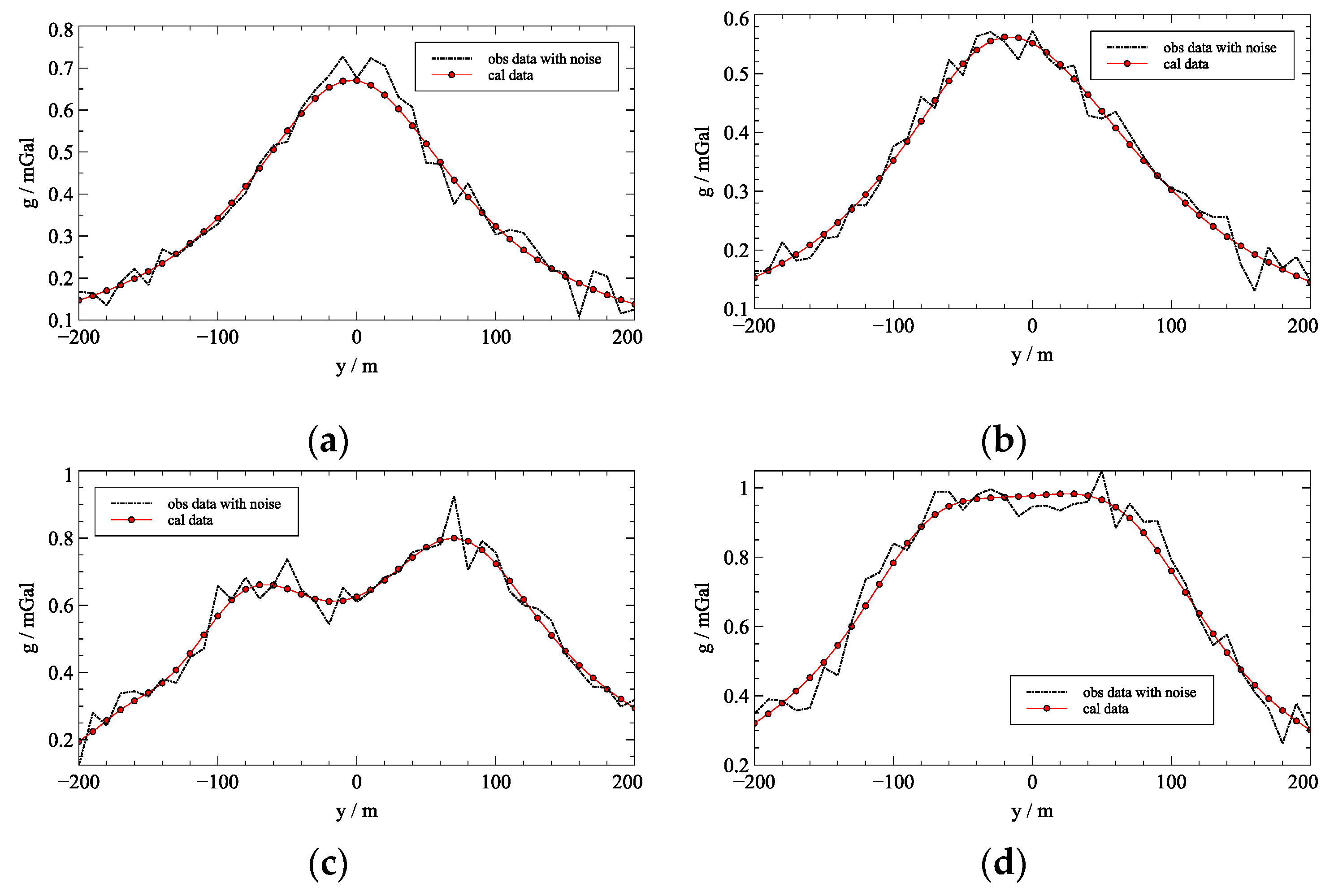
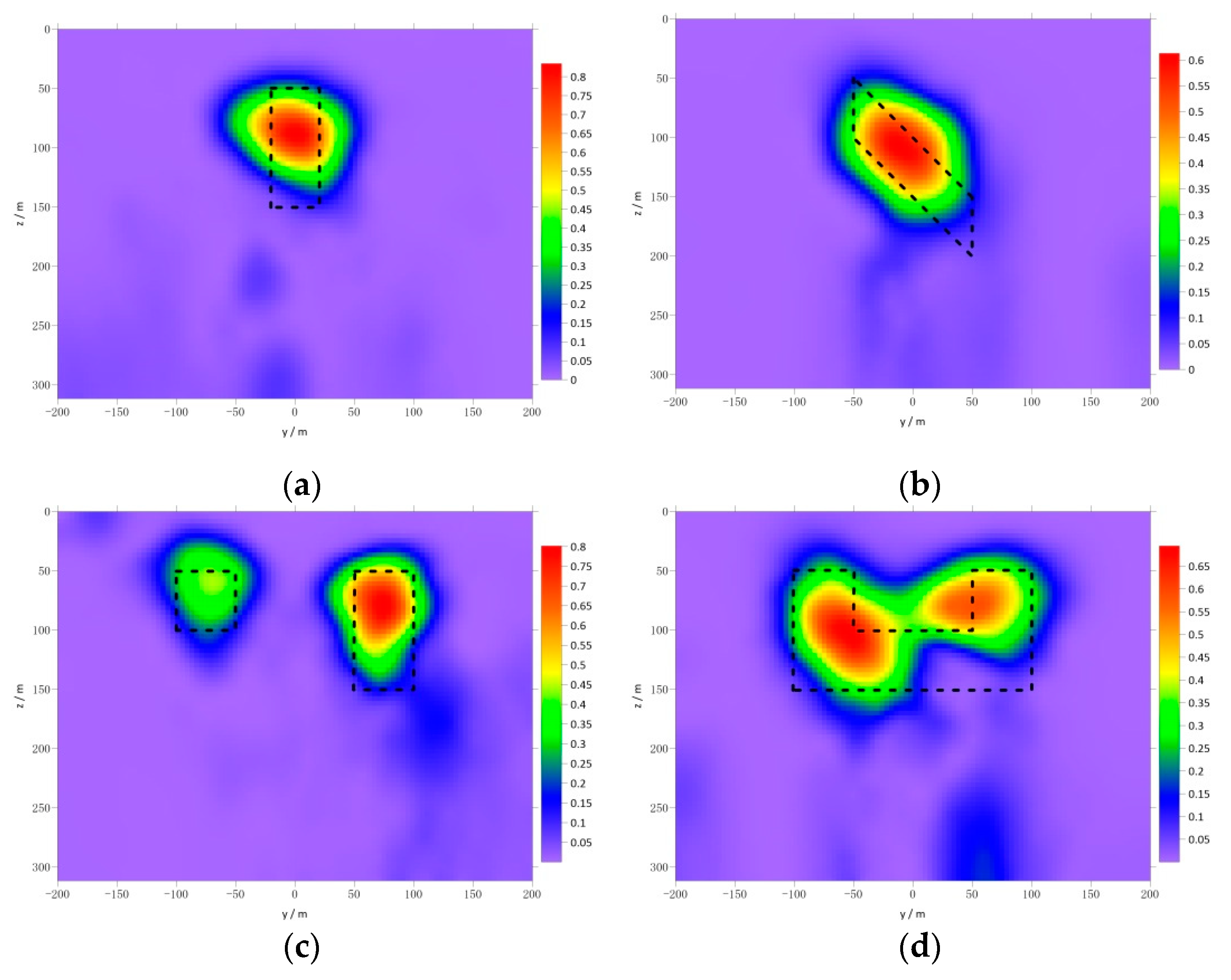
4.4. Gravity Data with Gaussian Noise
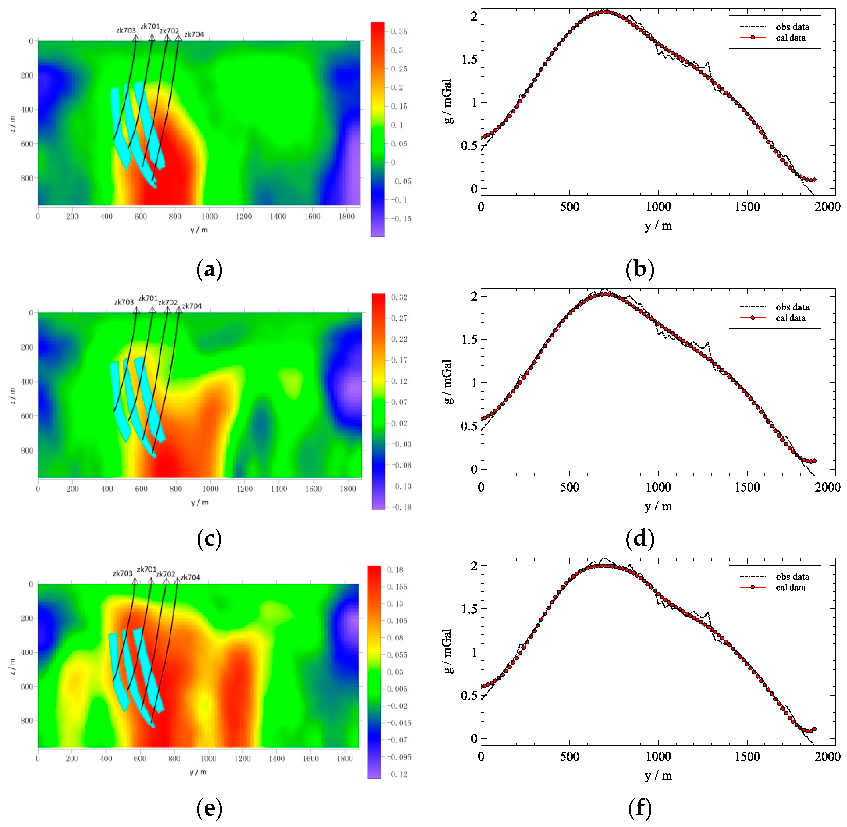
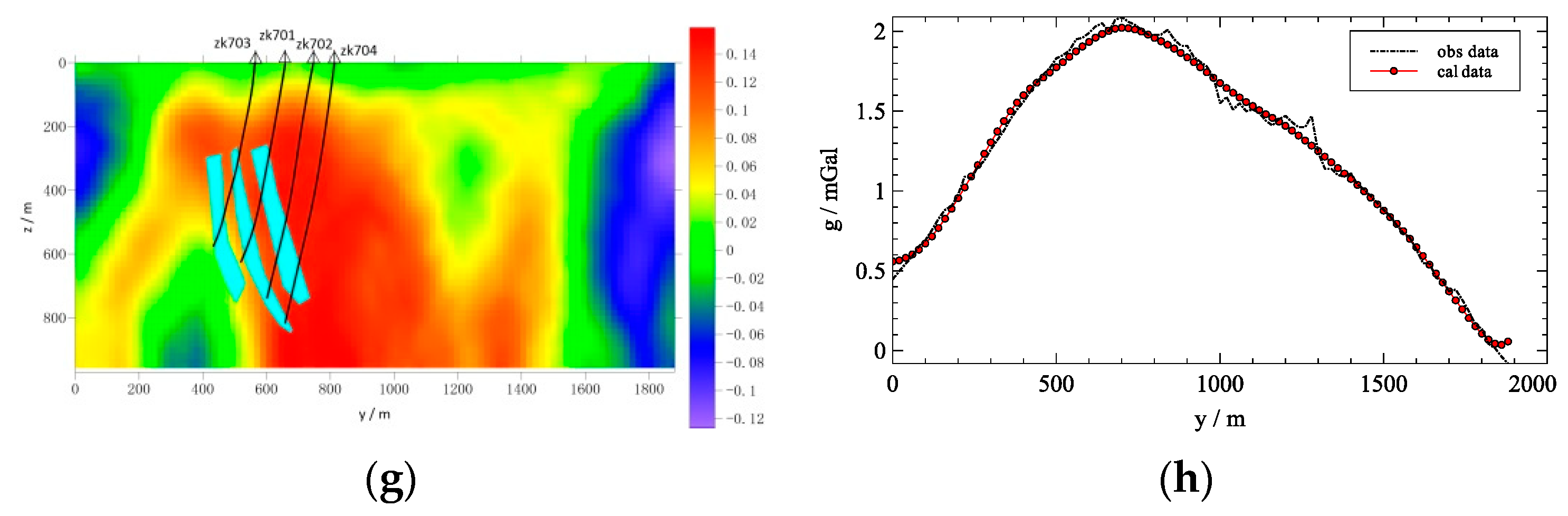
5. Field Example
6. Conclusions
Author Contributions
Funding
Institutional Review Board Statement
Informed Consent Statement
Data Availability Statement
Conflicts of Interest
References
- Paterson, N.R.; Reeves, C.V. Applications of gravity and magnetic surveys: The state-of-the-art in 1985. Geophysics 1985, 50, 2558–2594. [Google Scholar] [CrossRef]
- Li, Y.; Oldenburg, D.W. 3-D inversion of gravity data. Geophysics 1998, 63, 109–119. [Google Scholar] [CrossRef]
- Fullagar, P.K.; Pears, G.; Hutton, D.; Thompson, A. 3D gravity and aeromagnetic inversion for MVT lead-zinc exploration at Pillara, Western Australia. Explor. Geophys. 2004, 35, 142–146. [Google Scholar] [CrossRef]
- Hinze, W.J.; Von Frese, R.R.; Saad, A.H. Gravity and Magnetic Exploration: Principles, Practices, and Applications; Cambridge University Press: Cambridge, UK, 2013. [Google Scholar]
- Afshar, A.; Norouzi, G.-H.; Moradzadeh, A.; Riahi, M.-A. Application of magnetic and gravity methods to the exploration of sodium sulfate deposits, case study: Garmab mine, Semnan, Iran. J. Appl. Geophys. 2018, 159, 586–596. [Google Scholar] [CrossRef]
- Montesinos, F.G.; Arnoso, J.; Vieira, R. Using a genetic algorithm for 3-D inversion of gravity data in Fuerteventura (Canary Islands). Int. J. Earth Sci. 2005, 94, 301–316. [Google Scholar] [CrossRef]
- Pallero, J.L.G.; Fernández-Martínez, J.L.; Fernández-Muñiz, Z.; Bonvalot, S.; Gabalda, G.; Nalpas, T. GravPSO2D: A Matlab package for 2D gravity inversion in sedimentary basins using the Particle Swarm Optimization algorithm. Comput. Geosci. 2021, 146, 104653. [Google Scholar] [CrossRef]
- Zhou, X. Gravity inversion of 2D bedrock topography for heterogeneous sedimentary basins based on line integral and maximum difference reduction methods. Geophys. Prospect. 2013, 61, 220–234. [Google Scholar] [CrossRef]
- Feng, J.; Meng, X.; Chen, Z.; Zhang, S. Three-dimensional density interface inversion of gravity anomalies in the spectral domain. J. Geophys. Eng. 2014, 11, 035001. [Google Scholar] [CrossRef]
- Feng, J.; Zhang, S.; Meng, X. Constraint 3D density interface inversion from gravity anomalies. Arab. J. Geosci. 2015, 9, 56. [Google Scholar] [CrossRef]
- Last, B.; Kubik, K.J.G. Compact gravity inversion. Geophysics 1983, 48, 713–721. [Google Scholar] [CrossRef]
- Shamsipour, P.; Marcotte, D.; Chouteau, M. 3D stochastic joint inversion of gravity and magnetic data. J. Appl. Geophys. 2012, 79, 27–37. [Google Scholar] [CrossRef]
- Meng, Z.-H.; Xu, X.-C.; Huang, D.-N. Three-dimensional gravity inversion based on sparse recovery iteration using approximate zero norm. Appl. Geophys. 2018, 15, 524–535. [Google Scholar] [CrossRef]
- Silva, J.B.C.; Teixeira, W.A.; Barbosa, V.C.F. Gravity data as a tool for landfill study. Environ. Geol. 2008, 57, 749. [Google Scholar] [CrossRef]
- Tarantola, A. Inverse Problem Theory: Methods for Data Fitting and Model Parameter Estimation; Elsevier: New York, NY, USA, 1987. [Google Scholar]
- Yu, P.; Wang, J.L.; Wu, J.S. An Inversion of Gravity Anomalies by Using a 2.5 Dimensional Rectangle Gridded Model and the Simulated Annealing Algorithm. Chin. J. Geophys. 2007, 50, 756–764. [Google Scholar] [CrossRef]
- Ekinci, Y.L.; Balkaya, Ç.; Göktürkler, G.; Turan, S. Model parameter estimations from residual gravity anomalies due to simple-shaped sources using Differential Evolution Algorithm. J. Appl. Geophys. 2016, 129, 133–147. [Google Scholar] [CrossRef]
- Yao, C.; Hao, T.; Guan, Z.; Zhang, Y. High-Speed Computation and Efficient Storage in 3-D Gravity and Magnetic Inversion. Chin. J. Geophys. 2003, 46, 351–361. [Google Scholar] [CrossRef]
- Storn, R.; Price, K. Differential Evolution–A Simple and Efficient Heuristic for global Optimization over Continuous Spaces. J. Glob. Optim. 1997, 11, 341–359. [Google Scholar] [CrossRef]
- Voratas, K. Comparison of Three Evolutionary Algorithms: GA, PSO, and DE. Ind. Eng. Manag. Syst. 2012, 11, 215–223. [Google Scholar]
- Kurban, T.; Civicioglu, P.; Kurban, R.; Besdok, E. Comparison of evolutionary and swarm based computational techniques for multilevel color image thresholding. Appl. Soft Comput. 2014, 23, 128–143. [Google Scholar] [CrossRef]
- Mohamed, A.W.; Hadi, A.A.; Mohamed, A.K. Gaining-sharing knowledge based algorithm for solving optimization problems: A novel nature-inspired algorithm. Int. J. Mach. Learn. Cybern. 2020, 11, 1501–1529. [Google Scholar] [CrossRef]
- Ilonen, J.; Kamarainen, J.-K.; Lampinen, J. Differential Evolution Training Algorithm for Feed-Forward Neural Networks. Neural Process. Lett. 2003, 17, 93–105. [Google Scholar] [CrossRef]
- Piotrowski, A.P. Differential Evolution algorithms applied to Neural Network training suffer from stagnation. Appl. Soft Comput. 2014, 21, 382–406. [Google Scholar] [CrossRef]
- Tang, Y.; Ji, J.; Zhu, Y.; Gao, S.; Tang, Z.; Todo, Y. A Differential Evolution-Oriented Pruning Neural Network Model for Bankruptcy Prediction. Complexity 2019, 2019, 8682124. [Google Scholar] [CrossRef] [Green Version]
- Yılmaz, O.; Bas, E.; Egrioglu, E. The Training of Pi-Sigma Artificial Neural Networks with Differential Evolution Algorithm for Forecasting. Comput. Econ. 2021. [Google Scholar] [CrossRef]
- Sheng, W.; Wang, X.; Wang, Z.; Li, Q.; Zheng, Y.; Chen, S. A Differential Evolution Algorithm with Adaptive Niching and K-Means Operation for Data Clustering. IEEE Trans. Cybern. 2020, 12, 1–15. [Google Scholar] [CrossRef] [PubMed]
- He, X.; Zhang, Q.; Sun, N.; Dong, Y. Feature Selection with Discrete Binary Differential Evolution. In Proceedings of the 2009 International Conference on Artificial Intelligence and Computational Intelligence, Shanghai, China, 7–8 November 2009; pp. 327–330. [Google Scholar]
- Zhenkui, P.; Yanli, Z.; Zhen, L. Image segmentation based on Differential Evolution algorithm. In Proceedings of the 2009 International Conference on Image Analysis and Signal Processing, Linhai, China, 11–12 April 2009; pp. 48–51. [Google Scholar]
- Ali, M.; Ahn, C.W.; Siarry, P. Differential evolution algorithm for the selection of optimal scaling factors in image watermarking. Eng. Appl. Artif. Intell. 2014, 31, 15–26. [Google Scholar] [CrossRef]
- Cuevas, E.; Zaldívar, D.; Perez-Cisneros, M. Image Segmentation Based on Differential Evolution Optimization. In Applications of Evolutionary Computation in Image Processing and Pattern Recognition; Cuevas, E., Zaldívar, D., Perez-Cisneros, M., Eds.; Springer International Publishing: Berlin/Heidelberg, Germany, 2016; pp. 9–22. [Google Scholar] [CrossRef]
- Bhandari, A.K.; Kumar, A.; Chaudhary, S.; Singh, G.K. A new beta differential evolution algorithm for edge preserved colored satellite image enhancement. Multidimens. Syst. Signal. Process. 2017, 28, 495–527. [Google Scholar] [CrossRef]
- Balkaya, Ç. An implementation of differential evolution algorithm for inversion of geoelectrical data. J. Appl. Geophys. 2013, 98, 160–175. [Google Scholar] [CrossRef]
- Li, H.; Wang, H.; Wang, L.; Zhou, X. A modified Boltzmann Annealing Differential Evolution algorithm for inversion of directional resistivity logging-while-drilling measurements. J. Pet. Sci. Eng. 2020, 188, 106916. [Google Scholar] [CrossRef]
- Ekinci, Y.L.; Özyalın, Ş.; Sındırgı, P.; Balkaya, Ç.; Göktürkler, G. Amplitude inversion of the 2D analytic signal of magnetic anomalies through the differential evolution algorithm. J. Geophys. Eng. 2017, 14, 1492–1508. [Google Scholar] [CrossRef]
- Balkaya, Ç.; Ekinci, Y.L.; Göktürkler, G.; Turan, S. 3D non-linear inversion of magnetic anomalies caused by prismatic bodies using differential evolution algorithm. J. Appl. Geophys. 2017, 136, 372–386. [Google Scholar] [CrossRef]
- Du, W.; Cheng, L.; Li, Y. lp Norm Smooth Inversion of Magnetic Anomaly Based on Improved Adaptive Differential Evolution. Appl. Sci. 2021, 11, 1072. [Google Scholar] [CrossRef]
- Wu, G.; Mallipeddi, R.; Suganthan, P.N.; Wang, R.; Chen, H. Differential evolution with multi-population based ensemble of mutation strategies. Inf. Sci. 2016, 329, 329–345. [Google Scholar] [CrossRef]
- Das, S.; Mullick, S.S.; Suganthan, P.N. Recent advances in differential evolution—An updated survey. Swarm Evol. Comput. 2016, 27, 1–30. [Google Scholar] [CrossRef]
- Zhang, J.; Sanderson, A.C. JADE: Adaptive Differential Evolution with Optional External Archive. IEEE Trans. Evol. Comput. 2009, 13, 945–958. [Google Scholar] [CrossRef]
- Tanabe, R.; Fukunaga, A. Success-history based parameter adaptation for Differential Evolution. In Proceedings of the 2013 IEEE Congress on Evolutionary Computation, Cancun, Mexico, 20–23 June 2013; pp. 71–78. [Google Scholar]
- Mazumder, S. Numerical Methods for Partial Differential Equations; Academic Press: New York, NY, USA, 2016. [Google Scholar]
- Rao, K.; Jain, S.; Biswas, A. Global Optimization for Delineation of Self-potential Anomaly of a 2D Inclined Plate. Nat. Resour. Res. 2021, 30, 175–189. [Google Scholar] [CrossRef]
- Sharma, S.P.; Biswas, A. Interpretation of self-potential anomaly over a 2D inclined structure using very fast simulated-annealing global optimization—An insight about ambiguity. Geophysics 2013, 78, WB3–WB15. [Google Scholar] [CrossRef]
- Chen, X.B.; Zhao, G.-Z.; Tang, J.; Zhan, Y.; Wang, J.J. The Adaptive Regularized Inversion Algorithm (ARIA) for Magnetotelluric Data. Chin. J. Geophys. 2005, 48, 1005–1016. [Google Scholar] [CrossRef]
- Zhdanov, M.S. Chapter 5-Nonlinear Inversion Technique. In Inverse Theory and Applications in Geophysics, 2nd ed.; Zhdanov, M.S., Ed.; Elsevier: Oxford, UK, 2015; pp. 129–177. [Google Scholar] [CrossRef]
- Wu, Y.; Lu, J.; Sun, Y. Genetic Programming Based on an Adaptive Regularization Method. In Proceedings of the 2006 International Conference on Computational Intelligence and Security, Guangzhou, China, 3–6 November 2006; pp. 324–327. [Google Scholar]
- Zhou, Y.; Yi, W.; Gao, L.; Li, X. Adaptive Differential Evolution with Sorting Crossover Rate for Continuous Optimization Problems. IEEE Trans. Cybern. 2017, 47, 2742–2753. [Google Scholar] [CrossRef]


| Mineral | Number of Specimens | Arithmetic Mean (g/cm3) |
|---|---|---|
| PlagioclAse amphibolite | 41 | 2.78 |
| Garnet Magnetite Quartzite | 30 | 3.16 |
| Biotite Granulite | 27 | 2.88 |
| Amphibole Plagioclase | 7 | 2.65 |
| Layer | Number of specimens | Arithmetic mean (g/cm3) |
| Quaternary system | 6 | 1.53 |
| Jingangku formation | 106 | 2.78 |
Publisher’s Note: MDPI stays neutral with regard to jurisdictional claims in published maps and institutional affiliations. |
© 2021 by the authors. Licensee MDPI, Basel, Switzerland. This article is an open access article distributed under the terms and conditions of the Creative Commons Attribution (CC BY) license (https://creativecommons.org/licenses/by/4.0/).
Share and Cite
Song, T.; Hu, X.; Du, W.; Cheng, L.; Xiao, T.; Li, Q. Lp-Norm Inversion of Gravity Data Using Adaptive Differential Evolution. Appl. Sci. 2021, 11, 6485. https://doi.org/10.3390/app11146485
Song T, Hu X, Du W, Cheng L, Xiao T, Li Q. Lp-Norm Inversion of Gravity Data Using Adaptive Differential Evolution. Applied Sciences. 2021; 11(14):6485. https://doi.org/10.3390/app11146485
Chicago/Turabian StyleSong, Tao, Xing Hu, Wei Du, Lianzheng Cheng, Tiaojie Xiao, and Qian Li. 2021. "Lp-Norm Inversion of Gravity Data Using Adaptive Differential Evolution" Applied Sciences 11, no. 14: 6485. https://doi.org/10.3390/app11146485
APA StyleSong, T., Hu, X., Du, W., Cheng, L., Xiao, T., & Li, Q. (2021). Lp-Norm Inversion of Gravity Data Using Adaptive Differential Evolution. Applied Sciences, 11(14), 6485. https://doi.org/10.3390/app11146485