
New Vector-Space Embeddings for Recommender Systems


Abstract
:1. Introduction
- Collaborative Filtering: These are referred to as “people-to-people correlation”. These systems recommend items for users based on other users with similar taste. Two types of collaborative filtering exist [4]:
- –
- User–user (user-based): items are recommended based on the ratings that users with similar tastes have given to these items.
- –
- Item–item (item-based): items are recommended based on the similarity between them. The similarity computation between items depends on users who have rated/purchased both of these items.
- Content-Based: Recommendations are suggested based on the user’s history of preferences and profile where the features of the items are taken into consideration. For example a user who liked or purchased a particular item with certain features/specifications and a certain price range is more likely to show interest in another item possessing similar features.
- Demographic: These systems categorize users and provide recommendations based on the demographic profile of the user, such as age, gender, country, occupation, and so forth. Users in the same demographic group tend to have similarities in their interests, as opposed to users in different demographic groups.
- Knowledge-Based: These systems use knowledge to construct relations between items and users’ needs and preferences. The recommendations are suggested based on how the item is beneficial to a certain user.
- Community-Based: These systems make use of the information available in social networks. Recommendations can also be considered as “people-to-people correlation”, but this time relying on the user’s network of friends.
- Hybrid: These systems combine different approaches from those mentioned above.
- For our “prediction” problem we have a novel modeling framework. We train an embedding whereby each user maps to a vector and each item maps to a vector in the same space. The users’ and items’ vectors train side by side, and user–item, user–user and item–item similarities can be taken into account;
- The proposed method possesses an explicit capability to model sentiment, such as likes/dislikes. This is because the vectors are placed in a spherical space. This allows it to directly tackle the polarity issue, that is, “like” (vectors will be near each other) and “dislike” (vectors are on opposite poles of the sphere). Sentiment feedback in the form of like/dislike is particularly prevalent in video channels and music subscription services;
- The algorithm has an incremental nature. This makes adding a user or an item require only a small computational load;
- Conventional methods, such as matrix factorization using SVD or otherwise, are computationally very expensive, especially since the number of users and the number of items can be several tens of thousands. Even though using gradient methods for cases of matrix sparsity can reduce the computational cost, this is still a challenge. At the very least, the storage of such a huge matrix is a problem;
- Rather than dealing with huge user vectors, such as in the neighborhood-based techniques, our proposed embedding method considers (user or item) vectors of dimensions 10, 20 or 50. All information is therefore efficiently compressed;
- The developed embedding model produces a performance competitive with the state-of-the-art conventional recommender systems.
2. Related Work
2.1. Matrix Factorization
2.2. Neighborhood-Based Collaborative Filtering
2.3. Word Embedding
3. Proposed Approach
3.1. General Approach
- Demographic similarities: For example users who have similar demographic features, such as age, gender, country, profession, and so forth, will have assigned target similarities some number close to 1, while users with only a fraction of the demographic features will have a low target similarity;
- Community-based: Users who are in similar social networks, such as being friends, will have a high target similarity, otherwise it is low;
- Purchase pattern similarities: The target similarity can be proportional to the amount of items in common in both users’ purchasing patterns.
- Rating similarities: For example, the user u gives a rating for an item i and this rating would be set as the target similarity . (A high rating will produce a large similarity and vice versa.) This way, we can predict how any user would rate an item, by simply computing the similarity as the dot product after training is complete. This is what we call “Prediction”;
- Purchase pattern based: The target similarity can be proportional to the amount of times the user u purchased this item i in previous purchases.
- Content-based: For example, items i and that are similar or related product-types and have similar features and/or have a similar price range would have a high target similarity ;
- Purchase pattern based: The target similarity is proportional to the number of times the items i and are purchased together by some user. This is what we call “Recommendation”.
- 1.
- Generate the initial vectors randomly, normalizing them as unit length.
- 2.
- For to N perform the following:
- 3.
- Fix all except and update as follows:where
- A is a matrix defined as:
- b is a vector defined as:
- is the scalar Lagrange multiplier, evaluated using a simple one-dimensional bisection search so that: .
- 4.
- Repeat Steps 2–3 until the vectors converge.
3.2. Prediction
- is the user’s vector.
- is the item’s vector.
- is the rating user u assigned to item i, fed to the system as the rating scaled value where the maximum value is 1.
- is a weighing coefficient that constraints the system, which is designed to put different emphases on different ratings terms. In most practical cases we take as constant or one, unless certain ratings are deemed more influential.
- U is the number of users.
- N is the number of items.
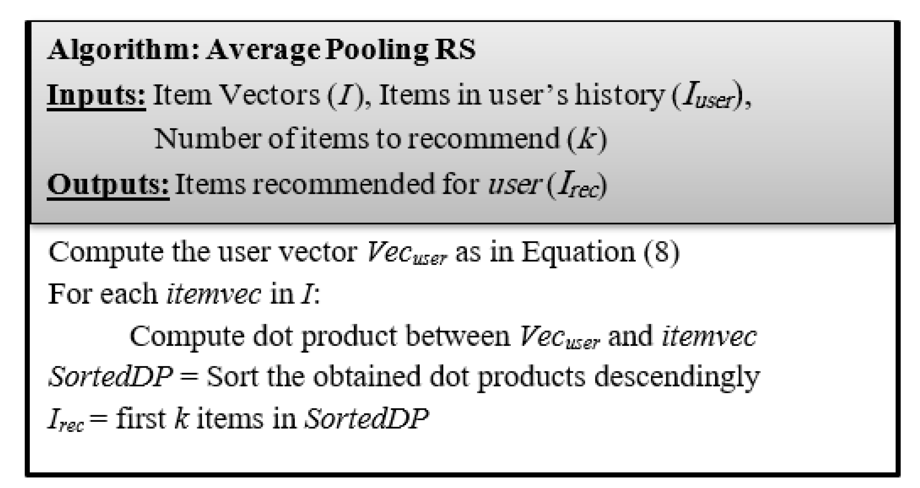
3.3. Recommendation
- x is the item’s vector.
- is a number proportional to the number of transactions where the items i and occur together, fed to the system as a scaled value where the maximum value is 1.
- is a weighing coefficient whose purpose is to put different emphases on different terms. Typically we take them to equal one.
- N is the number of items.
- is the vector of the item.
- T is the number of items in the user’s history.
4. Evaluation and Results
4.1. Prediction
- Applied 5-fold cross-validation.
- Five experiments were performed such that four folds were used as the training set and the remaining fifth fold was used as the test set, where in each experiment the folds were rotated as in the standard K-fold validation procedure.
- The training set consisted of the transactions fed to the vectors’ learning algorithm where users’ and items’ vectors of dimension 50 were learned for all the used datasets except the “Amazon MS” dataset where the vector’s dimension is only 10. The ratings in the given transactions were first normalized by dividing by five before being fed to the algorithm (so the maximum rating value became 1 and the minimum rating value became 0.2).
- The test set was the set used for performance evaluation by predicting the rating value for each transaction in the set. The prediction was performed by calculating the dot product between the user’s vector and the item’s vector involved in the transaction. Then, the obtained predicted rating was restored to the original ratings’ scale (for example by multiplying by 5).
- For each test set, two evaluation metrics were computed: Root Mean Square Error (RMSE) and Mean Absolute Error (MAE) [45]., where Q is the test set, is user u’s true rating given to item i and is the predicted rating of the Recommender System.
- The mean value for each metric RMSE and MAE was computed for all the five folds. This is the value recorded in the results.
- Singular Value Decomposition (SVD) [48]:SVD is the matrix factorization technique where the ratings matrix R (that includes users’ ratings for the items) is factored into three matrices as follows:, where U and V are orthogonal matrices of sizes and respectively.r is the rank of the rating matrix R.S is an diagonal matrix that includes all singular values of matrix R stored in descending order.The SVD approach is a kind of dimensionality reduction method and it provides the best lower rank approximations for the original matrix R. The matrix S can be reduced to by including only the largest k diagonal values. Consequently, U and V are reduced, obtaining . For user u and item i, the rating prediction is computed as the dot product between the u-th row of and i-th column of followed by adding the user average back.
- SVD++ [49]:This is an extension of the SVD approach, where implicit feedback is incorporated. An implicit feedback refers to the fact that a user u rated an item i without regard to the value of the given rating.
- Non-negative Matrix Factorization (NMF) [50]:This approach is similar to SVD; however, stochastic gradient descent (SGD) is used for the optimization procedure. SGD is carried out with a specific choice of step size ensuring the non-negativity of factors given that the factors’ initial values are positive.
- Slope One [51]:The technique relies on the SlopeOne algorithm, where predictors are used to compute the average difference between the ratings of one item and another for users who rated both. The rating prediction is defined as:, where is the average of ratings given by user u.is the set of relevant items: the set of items j rated by user u that also have at least one common user with i.is the number of elements in a set.is the average deviation of ratings of items i with respect to items j, given by:
- K-Nearest Neighbors (k-NN) [24]:The predictions of ratings are performed based on the ratings given by the user’s nearest-neighbors. In such models, known as memory-based models, the stored ratings are directly used in the prediction process.
- Centered k-NN [24]:This is a k-NN technique that takes into account the average ratings of each user to provide a corrective action to the prediction.
- k-NN Baseline [52]:This is a k-NN technique that incorporates baseline estimates. These estimates account for data tendencies such as the likelihood that some users give higher ratings than other users or that some items receive higher ratings than other items.
- Co-Clustering [53]:Clusters are built simultaneously for users and items. The predictions are based on the average ratings of the co-clusters (user–item neighborhoods). Formally, rating prediction is given as:, where is the average rating of co-cluster for user u and item i.is the average rating of user u’s cluster.is the average rating of item i’s cluster.
- Baseline [52]:In this technique, a simple baseline estimate is computed for the rating predictions, taking into account the aforementioned data tendencies. Formally, rating prediction is defined as:, where is the overall average rating.Parameters and are determined by solving a least squares problem.
4.2. Recommendation
- InvoiceNo: invoice number, which is a unique number identifying each transaction.
- StockCode: item/product code, which is a unique number identifying each product/item.
- Description: item/product descriptive name.
- Quantity: quantity of item/product per transaction.
- InvoiceDate: day and time of transaction.
- UnitPrice: price of item/product.
- CustomerID: customer number, which is a unique number identifying each customer.
- Country: country where customer resides.
- equals 1 if there is a hit for customer c and 0 otherwise. A hit is determined when at least one item in the set of recommended items matches one of the items in the true most recent transaction(s) of customer c.
- C is the total number of customers in the test set.
- As k increases, the “HitRate” increases, because there would be more chance that the user’s purchase is included in the recommended basket of items.
- Our approach outperforms word2vec for all k values.
5. Conclusions
Author Contributions
Funding
Conflicts of Interest
Appendix A. Complexity Analysis
- (a)
- Computing the matrix A according to Equation (4): The complexity is . Note that the summation is over existing ratings for user i, rather than over all items, so it is not a large summation.
- (b)
- Computation of b according to Equation (5) is .
- (c)
- Computation of Equation (3) is .
- (d)
- Computation of through the bisection search is , where B is the number of bisection search steps. Typically B is around 20.
- (e)
- Each of these computations is repeated N times (the total number of vectors or users and items).
- (f)
- Typically N is very large (several thousands), while M, the dimension of each vector is usually small (we take it as 10, 20 or 50). Using this fact and retaining only the largest terms, we get the amount of computation per cycle as approximately equal to .
- (g)
- The term (number of users times number of ratings per user plus number of items times number of ratings per item) is essentially twice the total number of ratings (twice because we count that from the users’ side and also from the items’ side).
- (h)
- So the total complexity per cycle is where K is the total number of ratings.
- (i)
- We have also implemented an accelerated version of the part that searches and computes using eigenvalue decomposition. This relieves us from solving the linear equations B times. The complexity of the search using bisection becomes instead of per cycle, i.e., better than the previous basic algorithm. So the total complexity per cycle becomes . The details are not given here to avoid distraction to algorithmic issues.
- (j)
- For the off-line algorithm, i.e., applying the algorithm from scratch to train all vectors the complexity equals the preceding times the number of cycles C, i.e., . Typically C is around 10 to 20. For the update phase, i.e receiving an extra rating or user and hence implementing only one cycle, the complexity becomes (for the eigenvalue search method).
- (k)
- The terms C, M, and B in the complexity formula are usually small, e.g., 10 to 50. The only impactful terms are K (the total number of ratings) and N (the total number of users plus items). These can for example be 100,000 or a million. What is important in the complexity analysis is that these terms (i.e., the K and the N) turned out to appear as linear terms, not more.
References
- Ortega, F.; González-Prieto, Á. Recommender Systems and Collaborative Filtering. Appl. Sci. 2020, 10, 7050. [Google Scholar] [CrossRef]
- Fayyaz, Z.; Ebrahimian, M.; Nawara, D.; Ibrahim, A.; Kashef, R. Recommendation Systems: Algorithms, Challenges, Metrics, and Business Opportunities. Appl. Sci. 2020, 10, 7748. [Google Scholar] [CrossRef]
- Ricci, F.; Rokach, L.; Shapira, B. Recommender systems: Introduction and challenges. In Recommender Systems Handbook; Springer: Boston, MA, USA, 2015; pp. 1–34. [Google Scholar]
- Sarwar, B.; Karypis, G.; Konstan, J.; Riedl, J. Item-based collaborative filtering recommendation algorithms. In Proceedings of the 10th International Conference on World Wide Web, Hong Kong, China, 1–5 May 2001; pp. 285–295. [Google Scholar]
- Sohail, S.S.; Siddiqui, J.; Ali, R. Classifications of Recommender Systems: A review. J. Eng. Sci. Technol. Rev. 2017, 10, 132–153. [Google Scholar] [CrossRef]
- Isinkaye, F.O.; Folajimi, Y.; Ojokoh, B.A. Recommendation systems: Principles, methods and evaluation. Egypt. Inform. J. 2015, 16, 261–273. [Google Scholar] [CrossRef] [Green Version]
- Gómez-Pulido, J.A.; Durán-Domínguez, A.; Pajuelo-Holguera, F. Optimizing Latent Factors and Collaborative Filtering for Students’ Performance Prediction. Appl. Sci. 2020, 10, 5601. [Google Scholar] [CrossRef]
- Yang, Z.; Wu, B.; Zheng, K.; Wang, X.; Lei, L. A survey of collaborative filtering-based recommender systems for mobile internet applications. IEEE Access 2016, 4, 3273–3287. [Google Scholar] [CrossRef]
- Zhang, S.; Yao, L.; Sun, A.; Tay, Y. Deep learning based recommender system: A survey and new perspectives. ACM Comput. Surv. 2019, 52, 1–38. [Google Scholar] [CrossRef] [Green Version]
- Bobadilla, J.; Alonso, S.; Hernando, A. Deep Learning Architecture for Collaborative Filtering Recommender Systems. Appl. Sci. 2020, 10, 2441. [Google Scholar] [CrossRef] [Green Version]
- Shafqat, W.; Byun, Y.C.; Park, N. Effectiveness of Machine Learning Approaches Towards Credibility Assessment of Crowdfunding Projects for Reliable Recommendations. Appl. Sci. 2020, 10, 9062. [Google Scholar] [CrossRef]
- Shafqat, W.; Byun, Y.C. Incorporating Similarity Measures to Optimize Graph Convolutional Neural Networks for Product Recommendation. Appl. Sci. 2021, 11, 1366. [Google Scholar] [CrossRef]
- Sulikowski, P.; Zdziebko, T. Horizontal vs. Vertical Recommendation Zones Evaluation Using Behavior Tracking. Appl. Sci. 2021, 11, 56. [Google Scholar] [CrossRef]
- Sulikowski, P.; Zdziebko, T.; Coussement, K.; Dyczkowski, K.; Kluza, K.; Sachpazidu-Wójcicka, K. Gaze and Event Tracking for Evaluation of Recommendation-Driven Purchase. Sensors 2021, 21, 1381. [Google Scholar] [CrossRef]
- Mikolov, T.; Chen, K.; Corrado, G.; Dean, J. Efficient estimation of word representations in vector space. arXiv 2013, arXiv:1301.3781. [Google Scholar]
- Mikolov, T.; Sutskever, I.; Chen, K.; Corrado, G.S.; Dean, J. Distributed representations of words and phrases and their compositionality. In Proceedings of the 26th International Conference on Neural Information Processing Systems—Volume 2 (NIPS’13), Lake Tahoe, NV, USA, 5–8 December 2013; Curran Associates Inc.: Red Hook, NY, USA, 2013; pp. 3111–3119. [Google Scholar]
- Koren, Y.; Bell, R.; Volinsky, C. Matrix factorization techniques for recommender systems. Computer 2009, 42, 30–37. [Google Scholar] [CrossRef]
- Yang, X.; Guo, Y.; Liu, Y.; Steck, H. A survey of collaborative filtering based social recommender systems. Comput. Commun. 2014, 41, 1–10. [Google Scholar] [CrossRef]
- Girase, S.; Mukhopadhyay, D. Role of matrix factorization model in collaborative filtering algorithm: A survey. arXiv 2015, arXiv:1503.07475. [Google Scholar]
- Ma, H.; Zhou, D.; Liu, C.; Lyu, M.R.; King, I. Recommender systems with social regularization. In Proceedings of the Fourth ACM International Conference on Web Search and Data Mining, Hong Kong, China, 9–12 February 2011; pp. 287–296. [Google Scholar]
- Guan, X.; Li, C.T.; Guan, Y. Matrix factorization with rating completion: An enhanced SVD model for collaborative filtering recommender systems. IEEE Access 2017, 5, 27668–27678. [Google Scholar] [CrossRef]
- Mitroi, B.; Frasincar, F. An elastic net regularized matrix factorization technique for recommender systems. In Proceedings of the 35th Annual ACM Symposium on Applied Computing, Brno, Czech Republic, 30 May–3 April 2020; pp. 2184–2192. [Google Scholar]
- Melville, P.; Sindhwani, V. Recommender systems. Encycl. Mach. Learn. 2010, 1, 829–838. [Google Scholar]
- Desrosiers, C.; Karypis, G. A comprehensive survey of neighborhood-based recommendation methods. In Recommender Systems Handbook; Springer: Boston, MA, USA, 2011; pp. 107–144. [Google Scholar]
- Bobadilla, J.; Ortega, F.; Hernando, A.; Gutiérrez, A. Recommender systems survey. Knowl.-Based Syst. 2013, 46, 109–132. [Google Scholar] [CrossRef]
- Martín-Vicente, M.I.; Gil-Solla, A.; Ramos-Cabrer, M.; Pazos-Arias, J.J.; Blanco-Fernández, Y.; López-Nores, M. A semantic approach to improve neighborhood formation in collaborative recommender systems. Expert Syst. Appl. 2014, 41, 7776–7788. [Google Scholar] [CrossRef]
- Subramaniyaswamy, V.; Logesh, R. Adaptive KNN based recommender system through mining of user preferences. Wirel. Pers. Commun. 2017, 97, 2229–2247. [Google Scholar] [CrossRef]
- Ayyaz, S.; Qamar, U. Improving collaborative filtering by selecting an effective user neighborhood for recommender systems. In Proceedings of the 2017 IEEE International Conference on Industrial Technology (ICIT), Toronto, ON, Canada, 22–25 March 2017; pp. 1244–1249. [Google Scholar]
- Akama, S.; Kudo, Y.; Murai, T. Neighbor Selection for User-Based Collaborative Filtering Using Covering-Based Rough Sets. In Topics in Rough Set Theory. Intelligent Systems Reference Library; Springer: Cham, Switzerland, 2020; Volume 168, pp. 141–159. [Google Scholar]
- Gutiérrez, L.; Keith, B. A systematic literature review on word embeddings. In International Conference on Software Process Improvement; Springer: Cham, Switzerland, 2018; pp. 132–141. [Google Scholar]
- Grbovic, M.; Radosavljevic, V.; Djuric, N.; Bhamidipati, N.; Savla, J.; Bhagwan, V.; Sharp, D. E-commerce in your inbox: Product recommendations at scale. In Proceedings of the 21th ACM SIGKDD International Conference on Knowledge Discovery and Data Mining, Sydney, NSW, Australia, 10–13 August 2015; pp. 1809–1818. [Google Scholar]
- Vasile, F.; Smirnova, E.; Conneau, A. Meta-prod2vec: Product embeddings using side-information for recommendation. In Proceedings of the 10th ACM Conference on Recommender Systems, Boston, MA, USA, 15–19 September 2016; pp. 225–232. [Google Scholar]
- Liang, D.; Altosaar, J.; Charlin, L.; Blei, D.M. Factorization meets the item embedding: Regularizing matrix factorization with item co-occurrence. In Proceedings of the 10th ACM Conference on Recommender Systems, Boston, MA, USA, 15–19 September 2016; pp. 59–66. [Google Scholar]
- Ozsoy, M.G. From word embeddings to item recommendation. arXiv 2016, arXiv:1601.01356. [Google Scholar]
- Krishnamurthy, B.; Puri, N.; Goel, R. Learning vector-space representations of items for recommendations using word embedding models. Procedia Comput. Sci. 2016, 80, 2205–2210. [Google Scholar] [CrossRef] [Green Version]
- Pennington, J.; Socher, R.; Manning, C. Glove: Global vectors for word representation. In Proceedings of the 2014 Conference on Empirical Methods in Natural Language Processing (EMNLP), Doha, Qatar, 25–29 October 2014; pp. 1532–1543. [Google Scholar]
- Barkan, O.; Koenigstein, N. Item2vec: Neural item embedding for collaborative filtering. In Proceedings of the 2016 IEEE 26th International Workshop on Machine Learning for Signal Processing (MLSP), Vietri sul Mare, Italy, 13–16 September 2016; pp. 1–6. [Google Scholar]
- Yang, Z.; He, J.; He, S. A collaborative filtering method based on forgetting theory and neural item embedding. In Proceedings of the 2019 IEEE 8th Joint International Information Technology and Artificial Intelligence Conference (ITAIC), Chongqing, China, 24–26 May 2019; pp. 1606–1610. [Google Scholar]
- Lu, N.; Ohsawa, Y.; Hayashi, T. Learning Sequential Behavior for Next-Item Prediction. In Proceedings of the Annual Conference of JSAI 33rd Annual Conference, Niigata, Japan, 4–7 June 2019; p. 3B4E203. [Google Scholar] [CrossRef]
- Barkan, O.; Caciularu, A.; Katz, O.; Koenigstein, N. Attentive Item2vec: Neural attentive user representations. In Proceedings of the ICASSP 2020—2020 IEEE International Conference on Acoustics, Speech and Signal Processing (ICASSP), Barcelona, Spain, 4–8 May 2020; pp. 3377–3381. [Google Scholar]
- Rizkallah, S.; Atiya, A.F.; Shaheen, S. A Polarity Capturing Sphere for Word to Vector Representation. Appl. Sci. 2020, 10, 4386. [Google Scholar] [CrossRef]
- Harper, F.M.; Konstan, J.A. The movielens datasets: History and context. Acm Trans. Interact. Intell. Syst. 2015, 5, 1–19. [Google Scholar] [CrossRef]
- Wan, M.; Ni, J.; Misra, R.; McAuley, J. Addressing marketing bias in product recommendations. In Proceedings of the 13th International Conference on Web Search and Data Mining, Houston, TX, USA, 3–7 February 2020; pp. 618–626. [Google Scholar]
- Ni, J.; Li, J.; McAuley, J. Justifying recommendations using distantly-labeled reviews and fine-grained aspects. In Proceedings of the 2019 Conference on Empirical Methods in Natural Language Processing and the 9th International Joint Conference on Natural Language Processing (EMNLP-IJCNLP), Hong Kong, China, 3–7 November 2019; pp. 188–197. [Google Scholar]
- Chen, M.; Liu, P. Performance Evaluation of Recommender Systems. Int. J. Perform. Eng. 2017, 13. [Google Scholar] [CrossRef]
- Hug, N. Surprise: A python library for recommender systems. J. Open Source Softw. 2020, 5, 2174. [Google Scholar] [CrossRef]
- Surprise. Available online: https://github.com/NicolasHug/Surprise (accessed on 29 January 2021).
- Sarwar, B.; Karypis, G.; Konstan, J.; Riedl, J. Application of Dimensionality Reduction in Recommender System A Case study; Technical Report; Minnesota Univ Minneapolis Dept of Computer Science: Minneapolis, MN, USA, 2000. [Google Scholar]
- Kumar, R.; Verma, B.; Rastogi, S.S. Social popularity based SVD++ recommender system. Int. J. Comput. Appl. 2014, 87, 33–37. [Google Scholar] [CrossRef]
- Luo, X.; Zhou, M.; Xia, Y.; Zhu, Q. An efficient non-negative matrix-factorization-based approach to collaborative filtering for recommender systems. IEEE Trans. Ind. Inform. 2014, 10, 1273–1284. [Google Scholar]
- Lemire, D.; Maclachlan, A. Slope one predictors for online rating-based collaborative filtering. In Proceedings of the 2005 SIAM International Conference on Data Mining, Newport Beach, CA, USA, 21–23 April 2005; pp. 471–475. [Google Scholar]
- Koren, Y. Factor in the neighbors: Scalable and accurate collaborative filtering. ACM Trans. Knowl. Discov. Data 2010, 4, 1–24. [Google Scholar] [CrossRef]
- George, T.; Merugu, S. A scalable collaborative filtering framework based on co-clustering. In Proceedings of the Fifth IEEE International Conference on Data Mining (ICDM’05), Washington, DC, USA, 27–30 November 2005; p. 4. [Google Scholar]
- Chen, D.D. Online Retail Dataset. 2015. Available online: https://archive.ics.uci.edu/ml/datasets/online+retail (accessed on 27 August 2020).


| Dataset | ||||
|---|---|---|---|---|
| Aspect | MovieLens 100 K | MovieLens 1 M | ModCloth | Amazon MS |
| Total number of ratings | 100,000 | 1,000,209 | 99,893 | 2375 |
| Number of users | 943 | 6040 | 44,784 | 348 |
| Number of items | 1682 | 3706 | 1020 | 157 |
| Maximum number of ratings by one user | 737 | 2314 | 250 | 30 |
| Minimum number of ratings by one user | 20 | 20 | 1 | 3 |
| Mean number of ratings by one user | 106 | 165.6 | 2.2 | 6.8 |
| Median number of ratings by one user | 65 | 96 | 1 | 6 |
| MovieLens 100 K | MovieLens 1 M | ModCloth | Amazon MS | |||||
|---|---|---|---|---|---|---|---|---|
| Approach | RMSE | MAE | RMSE | MAE | RMSE | MAE | RMSE | MAE |
| Sphere (our proposed method) | 0.923 | 0.738 | 0.857 | 0.684 | 1.165 | 0.783 | 1.03 | 0.605 |
| SVD | 0.934 | 0.737 | 0.873 | 0.686 | 1.056 | 0.828 | 0.971 | 0.724 |
| SVD++ | 0.92 | 0.722 | 0.862 | 0.673 | 1.06 | 0.829 | 0.941 | 0.689 |
| NMF | 0.963 | 0.758 | 0.916 | 0.724 | 1.2 | 0.948 | 1.035 | 0.759 |
| Slope One | 0.946 | 0.743 | 0.907 | 0.715 | 1.150 | 0.87 | 0.996 | 0.637 |
| k-NN | 0.98 | 0.774 | 0.923 | 0.727 | - | - | 1.156 | 0.771 |
| Centered k-NN | 0.951 | 0.749 | 0.929 | 0.738 | - | - | 0.958 | 0.611 |
| k-NN Baseline | 0.931 | 0.733 | 0.895 | 0.706 | - | - | 1.038 | 0.699 |
| Co-Clustering | 0.963 | 0.753 | 0.915 | 0.717 | 1.137 | 0.856 | 0.986 | 0.619 |
| Baseline | 0.944 | 0.748 | 0.909 | 0.719 | 1.041 | 0.82 | 1.002 | 0.766 |
| Random | 1.514 | 1.215 | 1.504 | 1.206 | 1.398 | 1.06 | 1.437 | 1.059 |
| k = 1 | k = 5 | k = 10 | k = 15 | k = 20 | |
|---|---|---|---|---|---|
| Sphere (our approach) | |||||
| Future Transactions = 1 | 0.186 | 0.435 | 0.524 | 0.602 | 0.665 |
| Future Transactions = 2 | 0.268 | 0.544 | 0.639 | 0.704 | 0.756 |
| word2vec | |||||
| Future Transactions = 1 | 0.098 | 0.306 | 0.447 | 0.516 | 0.573 |
| Future Transactions = 2 | 0.14 | 0.404 | 0.549 | 0.626 | 0.685 |
Publisher’s Note: MDPI stays neutral with regard to jurisdictional claims in published maps and institutional affiliations. |
© 2021 by the authors. Licensee MDPI, Basel, Switzerland. This article is an open access article distributed under the terms and conditions of the Creative Commons Attribution (CC BY) license (https://creativecommons.org/licenses/by/4.0/).
Share and Cite
Rizkallah, S.; Atiya, A.F.; Shaheen, S. New Vector-Space Embeddings for Recommender Systems. Appl. Sci. 2021, 11, 6477. https://doi.org/10.3390/app11146477
Rizkallah S, Atiya AF, Shaheen S. New Vector-Space Embeddings for Recommender Systems. Applied Sciences. 2021; 11(14):6477. https://doi.org/10.3390/app11146477
Chicago/Turabian StyleRizkallah, Sandra, Amir F. Atiya, and Samir Shaheen. 2021. "New Vector-Space Embeddings for Recommender Systems" Applied Sciences 11, no. 14: 6477. https://doi.org/10.3390/app11146477
APA StyleRizkallah, S., Atiya, A. F., & Shaheen, S. (2021). New Vector-Space Embeddings for Recommender Systems. Applied Sciences, 11(14), 6477. https://doi.org/10.3390/app11146477