Reactive Obstacle–Avoidance Systems for Wheeled Mobile Robots Based on Artificial Intelligence

Abstract

Obstacle–Avoidance robots have become an essential field of study in recent years. This paper analyzes two cases that extend reactive systems focused on obstacle detection and its avoidance. The scenarios explored get data from their environments through sensors and generate information for the models based on artificial intelligence to obtain a reactive decision. The main contribution is focused on the discussion of aspects that allow for comparing both approaches, such as the heuristic approach implemented, requirements, restrictions, response time, and performance. The first case presents a mobile robot that applies a fuzzy inference system (FIS) to achieve soft turning basing its decision on depth image information. The second case introduces a mobile robot based on a multilayer perceptron (MLP) architecture, which is a class of feedforward artificial neural network (ANN), and ultrasonic sensors to decide how to move in an uncontrolled environment. The analysis of both options offers perspectives to choose between reactive Obstacle–Avoidance systems based on ultrasonic or Kinect sensors, models that infer optimal decisions applying fuzzy logic or artificial neural networks, with key elements and methods to design mobile robots with wheels. Therefore, we show how AI or Fuzzy Logic techniques allow us to design mobile robots that learn from their “experience” by making them safe and adjustable for new tasks, unlike traditional robots that use large programs to perform a specific task.

1. Introduction

The great boom of technological advances in robotic and artificial intelligence has permitted the development of new systems combining different characteristics and allowing applications for a future world. Different types of robots can be found and classified according to environments such as mobile ground systems, mobile aerial systems, and water and underwater mobile systems. Wheeled mobile robots consist of robots with motion capacity through wheels into the environment.

Previous robots required research on navigation or obstacle avoidance, which are significant issues and challenging tasks for mobile robots; they must be able to navigate safely [1] in different circumstances, mainly to avoid a collision. Mobile robots are composed of mechanical and electronic parts: actuators, sensors, computers, power units, electronics, and so on. Depending on the environment in which the mobile robot will be implemented, two approaches can be identified [2]; the first one uses the global knowledge of the environment, this means that, at all times, the robot has information about its location, movements, obstacles, and the goal. The second approach uses local information retrieved by range sensors such as sonar, laser, infrared, ultrasonic sensors, video cameras, or Kinect.

For example, ultrasonic proximity sensors use a transducer to send and receive high-frequency sound signals. If a target enters the beam, then the sound is sent back to the sensor, causing the output circuit to turn on or off. One advantage [3] of these sensors is that they perform better at detecting objects that are more than one meter away. Light does not affect their operation as it does with other proximity devices. They have high precision detecting objects inside 5 mm. In addition, they can measure the distance through liquids and transparent objects. The pulse duration is proportional to the transducer distance and the object that reflects the closest sound [4]. Applications have been proposed with ultrasonic sensors; for example, the authors in [5] developed an array of ultrasonic sensors with sixteen pieces mounted on a mobile robot to perform real-time 2D and 3D mapping.

Another sensor widely used in obstacle avoidance applications is the Microsoft Kinect sensor, which has become one of the most popular depth sensors for research purposes [6], created to recognize the human gesture in a game console and released in November 2010. The Kinect sensors use two devices to generate depth images: (1) An RGB Camera and (2) a 3D depth Sensor. The first one is the USB video camera ($640\times 480$) that performs facial recognition, object detection, and tracking; the second one is a 3D Depth Sensor formed by two devices: (a) an infrared laser projector and (b) a monochrome CMOS camera pair. The infrared laser projector (transmitter) incorporates an illumination light unit that projects a structured pattern light onto the objective scene and infers depth from that pattern’s deformation. A monochrome CMOS camera (receiver) takes this image from a different point and triangulates to obtain depth information, calculated at each RGB camera pixel.

Developing motion models is necessary, along with sensors and navigation. Models are developed based on robot kinematics and locomotion, which means moving an autonomous robot between two places. The kinematic model describes the relationship among inputs, parameters, and system behavior, describing the velocities through second-order differential equations. Different works proposing models for wheeled mobile robots appear in [7,8]. Authors in [9] presented a kinematic modeling scheme to analyze the skid-steered mobile robot. Their results show that the kinematic modeling proposed is useful in a skid-steered robot and tracked vehicles. In [10], a dynamic model for omnidirectional wheeled mobile robots is presented. According to the results, this model considers slip between wheels and motion surface. The friction model response is improved by considering the rigid material’s discontinuities among the omnidirectional wheel rollers. On the other hand, mobile robot models are based on different characteristics, such as structure and design. One characteristic consists of the kinematics of wheeled mobile robots. There are different types of kinematics: internal, external, direct, and inverse. The kinematic describes the relationship between mobile and the robot internal and external variables as a function of inputs and the environment.

During the last few years, several types of research are applying artificial intelligence to solve problems in different fields, such as engineering, finance, marketing, health, gaming, telecommunications, transportation, and many others. Obstacle avoidance for mobile robots has not been an exception. Authors in [11] developed a hybrid AI algorithm combining Q-learning and Autowisard that will permit an autonomous mobile robot to self-learn. Using five layers Neuro-fuzzy architecture to learn the environment and the navigation map of a place, the mobile robot was routed based wholly on the sensor input (3D vision) by [12].

In this paper, we extend and analyze two systems designed for Obstacle–Avoidance implemented to perform in real-world scenarios [13,14]. The first system [13] presents the case of a mobile robot that applies fuzzy logic to realize soft turns basing its decision on depth image information obtained by a Microsoft Kinect device; the second system [14] introduces the case of a mobile robot based on a multi-layer perceptron, navigating in an uncontrolled environment with the help of ultrasonic sensors to decide how to move. The main contribution of this work lies in the discussion of aspects learned through the experience of designing and implementing these mobile robots in real-world conditions, which allow comparing both approaches in terms of different considerations, such as the heuristic approach implemented, requirements, restrictions, response time, and performance. Although several works have approached this kind of comparison, such as the ones presented in [15,16], there is valuable information that a detailed discussion on environmental inputs and general operational conditions, along with the analysis of both options, can offer to help in the decision of selecting one approach or the other. Hence, this kind of analysis and discussion offers perspectives to choose: (i) between reactive Obstacle–Avoidance systems based on ultrasonic or Kinect sensors, and (ii) between models that infer optimal decisions applying fuzzy logic or artificial neural networks; with elements and methods that are key when designing wheeled mobile robots.

In the next sections, we present a brief explanation of two widely used AI techniques applied to mobile robots and some critical considerations and methods for obstacle avoidance and navigation applications.

2. Artificial Intelligence, Obstacle Avoidance, and Navigation

Heuristic approaches, such as Fuzzy Systems and Artificial Neural Networks (ANN), have been widely used in mobile robot navigation. The use of fuzzy logic is primarily seen to deal with uncertainty in sensory data [17].

Fuzzy Logic enables expert systems based on rules, which work closer to the “common sense” that humans apply to make decisions; these systems use fuzzy rules and fuzzy inference instead of exact rules. These rules intend to be subjective, ambiguous, vague, or contradictory, like the human common sense knowledge, acquired over the long-term and many people’s experiences, over many years [18].

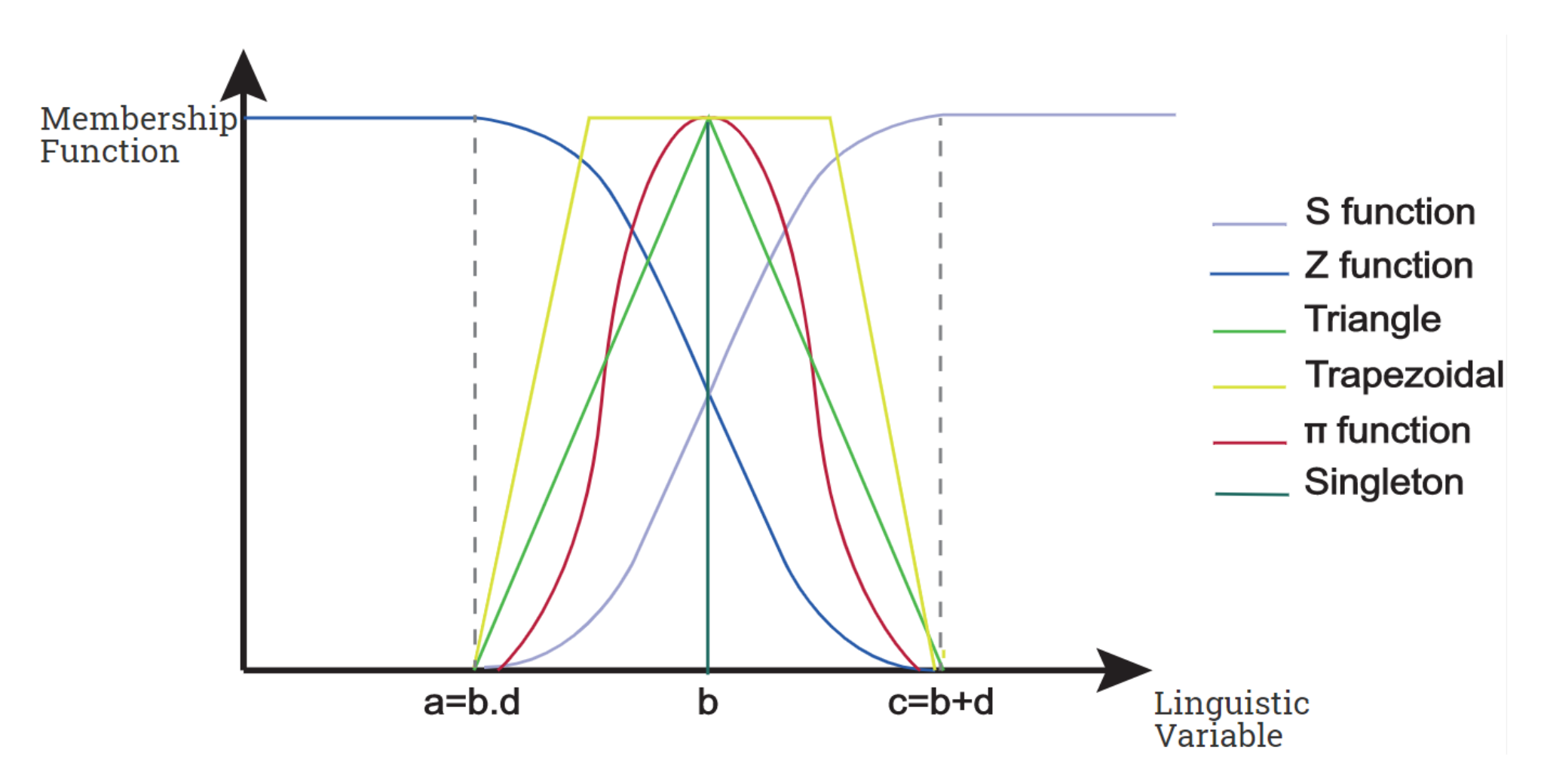
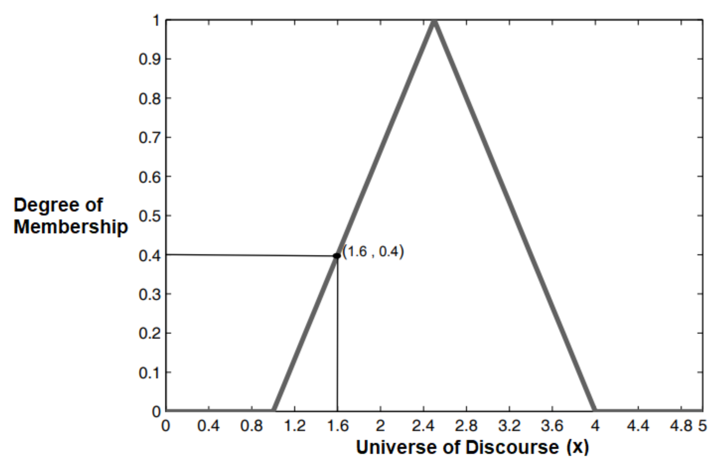
Fuzzy rules deal with fuzzy values, for example, “high”, “cold”, “very good”, etc. These concepts are usually represented by their membership functions, which show the extent to which a value from a domain is included in a fuzzy concept (see Figure 1). The knowledge of a specialist is necessary to define these rules and the regions of the membership functions. Fuzzy inference takes inputs, applies the rules, and produces outputs. Inputs to a fuzzy system can be either exact, crisp values, or fuzzy values (“very cold”); output values can be fuzzy, for example, a whole membership function for the inferred fuzzy value, or exact, for example, crisp values. The process of transforming an output membership function into a single value is called defuzzification.

Usually, a fuzzy system consists of the following steps [1]: (i) Fuzzification: where inputs are fuzzified to be associated with linguistic variables using membership functions. (ii) Inference: this refers to the fuzzy rule base containing fuzzy IF-THEN rules to derive the linguistic values for the intermediate and output linguistic variables. (iii) Defuzzification: once the output linguistic values are obtained, the defuzzification produces the final crisp values from the output linguistic values.

Several fuzzy logic applications exist in the market now, like control of automatic washing machines, camera focusing, control of transmission in cars, and many automation tasks such as landing systems and control of subways.

Many reactive navigation systems based on fuzzy control and ANN have been proposed over the last years, applying different input data types. For example, the authors in [19] use an IR transmitter and receiver to find the obstacle in the path of the vehicle, where they implement a multilayer feed-forward neural network with backpropagation training algorithms running inside a microcontroller. A neural network approach equipped with statistical dimension reduction techniques was created by [20] to increase the speed and precision of the network learning; authors used a feed-forward ANN based on function approximation with backpropagation training. Two different datasets, obtained from a laser range sensor, were used for training the networks. Development using Q-learning and a neural network planner was applied to solve path planning problems, which has proven to be effective in navigation scenarios where global information is available [2]. Even hybrid systems using Fuzzy Logic and ANNs have been proposed, like [1], where Fuzzy Logic treats the data of infrared sensors, which become the input of the ANN that decides which movement the robot must perform.

Artificial Neural Networks are an attempt to emulate the human brain neuron performance. Its structure can be defined by three layers: input layer, hidden layer, and output layer. ANNs can be classified by their topology (single layer or multi-layer) and its learning types (supervised, unsupervised, reinforcement, etc.) [17,21,22].

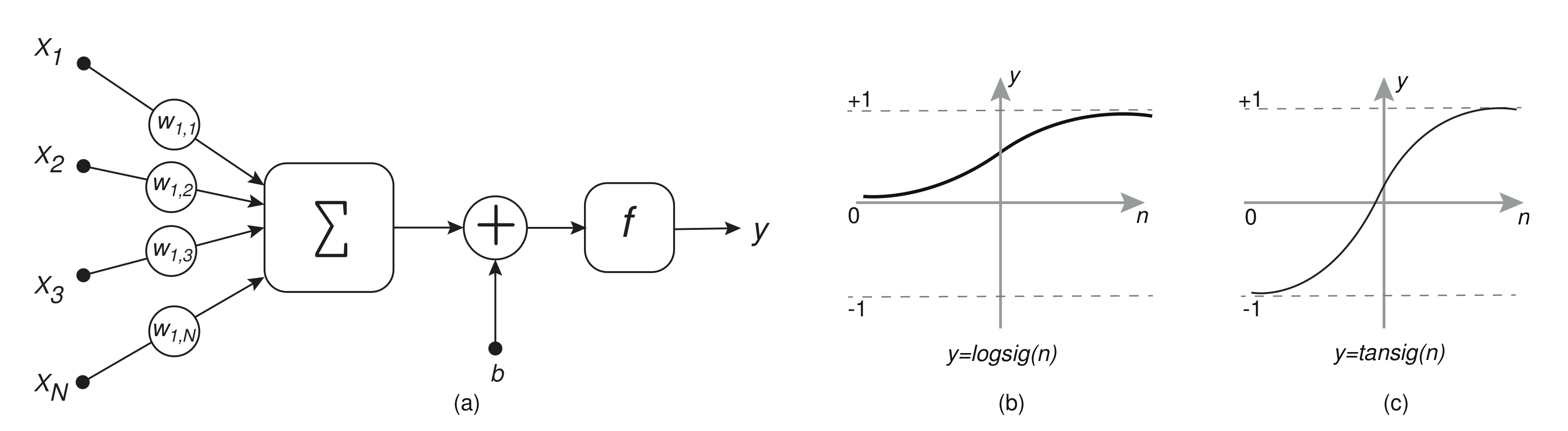
A single-layer network can have one or more inputs and outputs. As an example, Figure 2a shows a single-layer architecture with four inputs and one output. The individual inputs $x_1,x_2,x_3,\dots ,x_N$ are each weighted by its corresponding elements $w_{1,1},w_{1,2},w_{1,3},\dots ,w_{1,N}$ of the weight matrix $\mathbf{W}$. The bias neuron is added with the weighted inputs to create the net input (see Equation (1)):

$$n=w_{1,1}{x}_1+w_{1,2}{x}_2+w_{1,3}{x}_3+\dots +w_{1,N}{x}_N+b$$

(1)

In matrix form, Equation (1) will become as described in Equation (2), where matrix $\mathbf{X}$ stands for the input matrix:

$$n=\mathbf{W}\ast \mathbf{X}+\mathbf{b}$$

(2)

Finally, the neuron output can be written as in Equation (3):

$$y=f\left(\mathbf{W}\ast \mathbf{X}+\mathbf{b}\right)$$

(3)

where b represents the bias, and f is a transfer function (see Figure 2b,c) that is chosen depending on the application; this function will adjust the parameters w and b, depending on the learning rules, all this to achieve a specific input/output relationship.

An important characteristic that must be chosen when an ANN is designed is its transfer function (f). The selection is made from two possibilities: (a) linear will not limit the output of the functions between any range, or (b) nonlinear makes it easier for the model to adapt to data diversity, and it can differentiate among the outputs. The objective of the transfer function (also known as transformation, activation, or threshold function) is to avoid outputs from reaching very large values that can stop ANN and inhibit training [23]. A variety of transfer functions exist, such as hard limit transfer, symmetrical hard limit, log-sigmoid, and hyperbolic tangent sigmoid.

In this case, log-sigmoid transfer function $f=\frac{1}{1+e^{-n}}$ is one of the most used on ANN applications, which takes the input $(\pm 1)$ and adjusts the output into the range 0 to 1 (see Figure 2b), because it is a differentiable function and is commonly applied in multilayer networks trained with backpropagation [24]. Additionally, hyperbolic tangent sigmoid transfer function $f=\frac{e^n-e^{-n}}{e^n+e^{-n}}$ is related to a bipolar sigmoid that has an output in the range of (±) (see Figure 2c). This function is a good trade-off, where speed is more important than the transfer function’s exact shape.

Two principal architectures can be distinguished for ANNs:

• Feed forward network: Information travels in one direction between layers (input, hidden, and output) without affecting the past, present, or future layer. In other words, feedback between layers does not exist.
• Recurrent network: This network at least has one loop or feedback, allowing for storing information about its past calculations. Their capability to model temporal sequences of input–output pairs has given them success in natural language processing (NLP) applications: machine translation, speech recognition, and language modeling.

The ANNs can also be classified based on their learning/training types [18]:

• Supervised learning: On this training, each input is associated with an output, which will be the desired output (target). The training process is performed until the network “learns” to associate each input to its corresponding and desired output.
• Unsupervised learning: In this case, only the input is supplied to the network; the network learns by itself, adapting some internal features of the input presented a priori.
• Reinforcement learning: Here, a set of inputs is presented to the network; if the output provided by the network is “ok”, then the connection weights are increased (reward); otherwise, the weights decrease (penalty). This learning type is also known as “reward–penalty learning”.

One of the most used ANN architectures is the Multi-Layer Perceptron (MLP), a feed-forward ANN; it can have any number of inputs and one or more hidden layers. It generally applies linear combination functions on its input layers and has some number of outputs with any activation function.

Nowadays, ANNs are widely used in machine learning applications, such as autonomous navigations, where different types of inputs are provided, as images and distance measures.

Obstacle avoidance and navigation. It is one of the main tasks performed by mobile robots; it consists of avoiding a set of obstacles through the path to reach the goal in the environment. There are two techniques for obstacle avoidance on path planning: global and local. A global type requires full knowledge of the static environment to search the target from an initial place. The local strategy consists of detecting the robot’s position and obstacles close to it. In addition, for obstacle avoidance, two aspects need to be considered; the first one consists of detecting different obstacles through sensors. Second, the mobile robot will choose a proper path to reach the target without a crash.

The knowledge of the environment is an essential aspect to avoid obstacles. There are dynamic and static types of obstacles, which are obstacles moving and without changes, respectively. A set of parameters determines the robot’s position in space. Considering the parameters, a configuration is needed; this means that a system state at the environment space covered in n dimensions. Therefore, a vector space can be expressed by ${[q_1,\dots ,q_n]}^T$, where q is a point in the dimensional space Q [25].

In addition, robot navigation means finding its location and building a path to reach a goal, avoiding different environmental situations such as obstacles, radiation, weather, among others. Several approaches have been proposed to solve the autonomous navigation problem, such as methods based on fuzzy logic, neural networks, genetic algorithms, fuzzy-PSO, FLC-Expert systems, among others. For example, in [26], the authors proposed a method based on a combination of different algorithms, including fuzzy-PSO and genetic algorithms, to identify the optimal navigation in complex environments. According to their results, the proposal is suitable for navigation with and without obstacle avoidance in different environments.

Different techniques can represent the environment, such as graph representation, cell decomposition, and road-map, among others. For example, the environment representation can usually be translated into a graph containing all mobile robot stages and the area covered by obstacles. This graph is called a state transition graph when all intermediate configurations and transitions are considered.

Reactive methods need an accuracy system based on sensors that can avoid obstacles in the environment. One manner of performing is path planning, which is about tracking a path to guide the robot from an initial location to an objective. Usually, when path planning is performed, a map is used, and memory contains the data employed to build it. The main steps performed during path planning are: self location, path planning, map building, and map interpretation [27]. A useful path consists of a set of actions that guides the robot through two points. According to the problem’s target, an optimal path needs to satisfy different conditions such as smooth motion, constraints related to the problem, time used to reach the goal, and obstacle avoidance. In addition, motion planning is the process of selecting inputs and motions satisfying all constraints such as risk and obstacle avoidance. This task is performed through different models and environments [27].

3. System Analysis

In this section, two cases of obstacle avoidance with mobile robots are extended and analyzed. The two cases [13,14] apply different approaches from artificial intelligence: fuzzy logic and artificial neural networks, and their input signals are different as well.

3.1. Case I: Mobile Robot and Fuzzy Logic

The first case is a self-navigating robot, which uses depth data obtained from the Kinect sensor, and provides knowledge from its working space. This information enables us to adjust soft turning angles by applying fuzzy rules. The robotic system considers uncertain information aiming to provide services to disabled people to improve their quality of life.

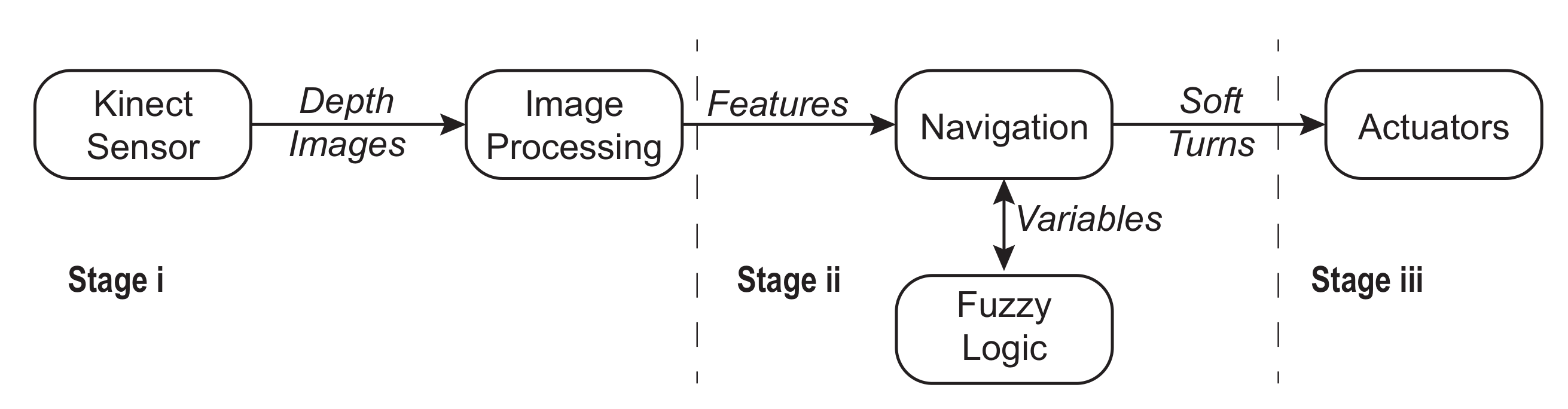
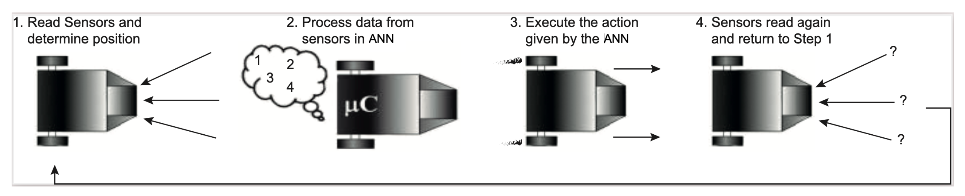
The architecture is reactive for soft turning and consists of three main stages: (i) data acquisition and processing, (ii) decision on navigation using fuzzy logic, and (iii) reactive behavior and actuators (see Figure 3). The first stage includes sensors (provide data) and data processing (generates features, metrics, and characteristics). The second stage takes processed data from the previous stage, which are inputs for the navigation module, based on fuzzy logic that generates certain decisions for the next stage. Finally, the third stage makes decisions and produces control signals for the mobile robot actuators, avoiding obstacles. These three stages provide the architecture with flexibility, adaptability, and fast-response capacity in front of unexpected situations. The main characteristics of the system are a depth image and fuzzy logic. The first one offers data and objects in a depth context, whereas the second one implements a fuzzy reactive inference control without the system model’s preconditions. In this way, the planning strategy is reactive and adjusts the wheels’ turning angle by sensing its environment in real time.

The mobile robot is designed and programmed to operate in a dynamic environment, which implies no environmental constraints. The architecture does not require a priori knowledge about the obstacles or their motion. The environment is dynamic, an important issue that many works do not consider because it implies that the environment changes and objects move. These objects must be recognized, and the robot must react in a short time to avoid them.

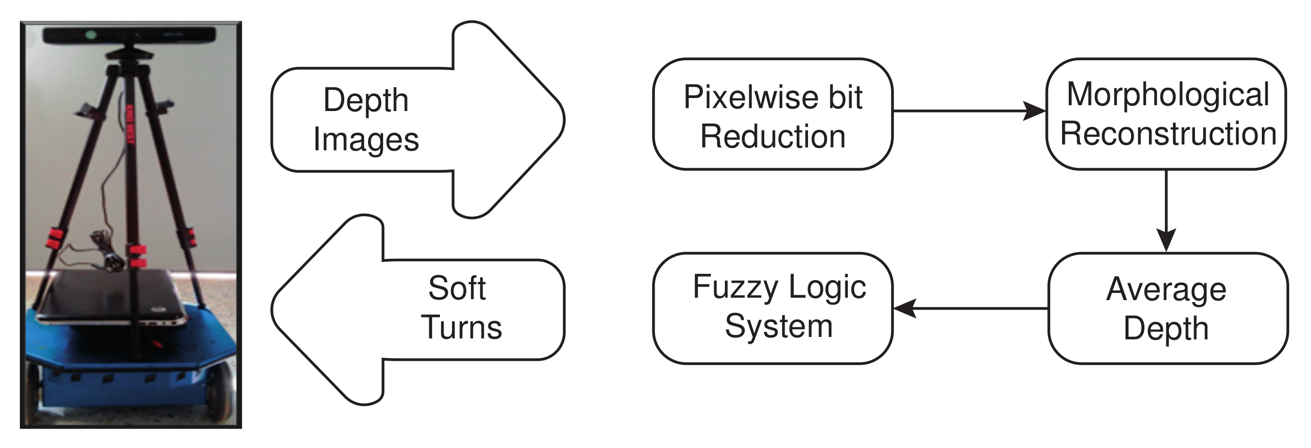
The Kinect sensor provides depth data, which is processed in a computer in four stages to generate the soft turning angle, avoiding future and unexpected collisions. The system was implemented and tested on the differential-type wheeled robot Era-Mobi equipped with an on-board computer and Wi-Fi antenna. The turning angle is sent to the robot via sockets using the Player/Stage server, a popular open-source generic server employed in robotics to control sensors and actuators. The Era-Mobi robot is compatible with a broad range of sensors, including infrared, sonar, laser telemeter, and stereoscopic vision. The analyzed system is integrated by four modules that transform depth data from the Kinect sensor into a soft turning angle (see Figure 4) described in the next sections.

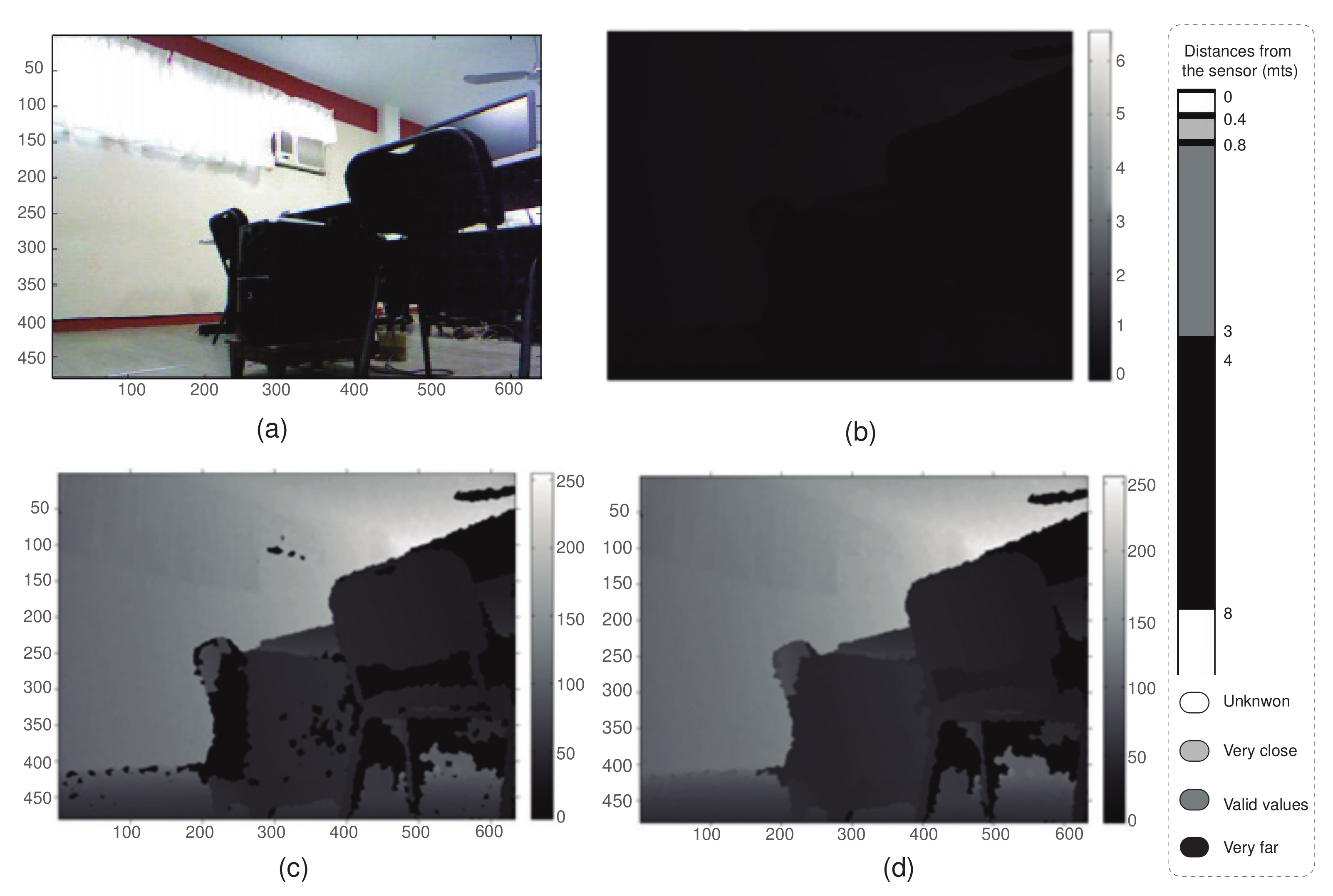
Module 1: Pixel-wise bit reduction. This module is based on depth images acquired using the Kinect sensor, which has a size of 640 × 480 pixels. On the one hand, Figure 5a presents an RGB image, which is shown for visual reference and is not used for processing or analyzing. On the other hand, depth images are processed, where each pixel represents a depth value in a range between 0 millimeters (black color) and 65,535 millimeters (white color), as can be seen in Figure 5b. In this image, most pixels fall into the darker specter, since they are in an extreme vision range of the Kinect sensor (about 10,000 millimeters). The pixel-wise reduction process transforms the 16-bit image (format from the Kinect sensor) into an 8-bit image (see Figure 5c), where 0-value represents a distance very close, very far or unidentified objects. Thus, the navigation system must maintain a path towards places where there is enough space, avoiding going towards regions where 0-values are predominant and, consequently, avoiding potential future collisions. Otherwise, the system stops the actuators.

Module 2: Morphological reconstruction. To simplify data in images, morphology can offer this process, keeping essential features and suppressing those aspects that are irrelevant. The system searches depth features and, at the same time, removes small unknown regions surrounded by known regions, providing a higher definition from the objects and their depth into the environment. Specifically, this module uses the geodesic erosion algorithm, highlighting those pixels with the lowest sharpness whenever their neighboring pixels are sharper, providing depth images with a lower amount of dark particles. Figure 5d shows a depth image, which has been processed by the morphological reconstruction.

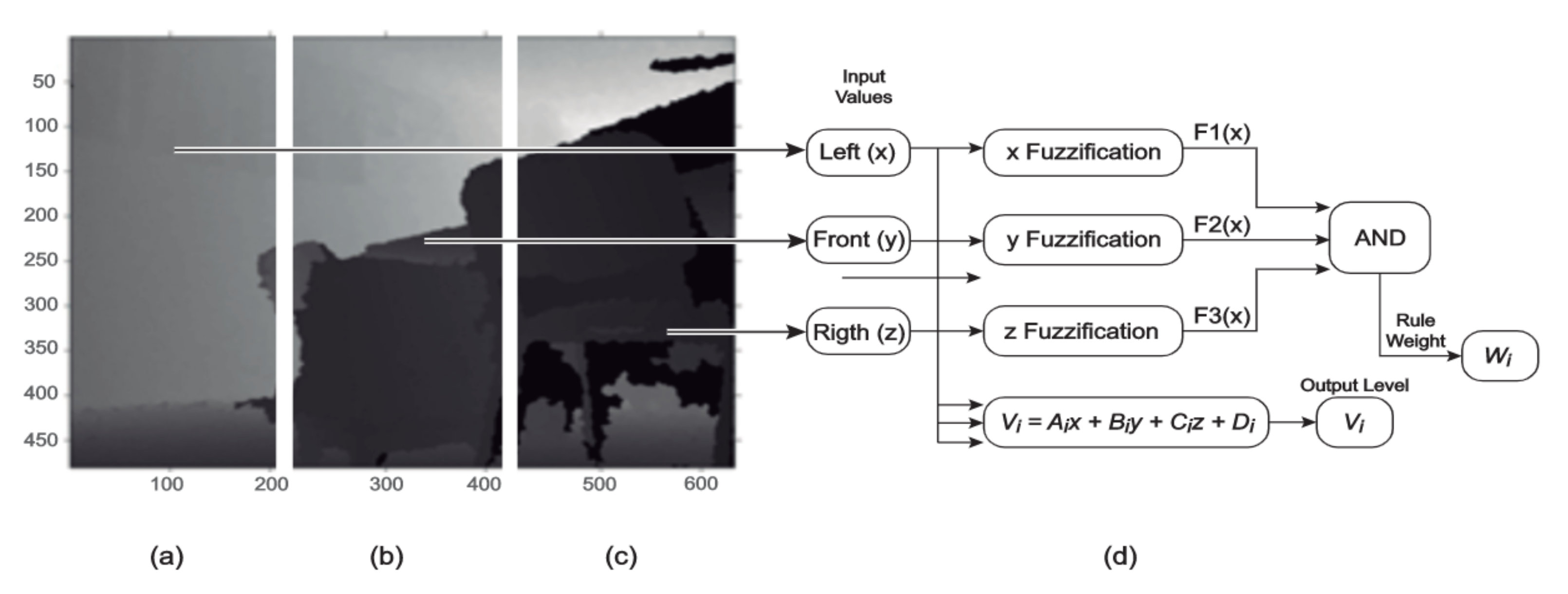
Module 3: Average depth. In this context, the robot can go to different places, and the system takes into account the work volume of the robot. Thus, the depth image processed by the previous module is divided into Left Subimage, Center Subimage, and Right Subimage (see Figure 6a–c) [28]. Each sub-image has a size of 211 × 400 pixels, representing the possible reference paths where the mobile platform can go: turn right, forward, and turn left. This division is computed by two factors: (1) the dimensions of the mobile robot (length = 400 millimeters, width = 410 millimeters, and height = 150 + 630 millimeters, where 150 millimeters are due to the physical robot and 630 millimeters are due to the Kinect sensor and its support) and (2) the sensed effective distance by the Kinect sensor (about 3000 millimeters).

The module implements the method proposed by [29], computing the threshold value and differentiating high and low depths. For each sub-image, if the amount of unknown data (0-values) is more considerable than a given percentage (67% in this case), the sub-image data suggest nearby obstacles, and the average depth is computed by using the mean of the low-valued depths. Otherwise, the average depth is computed by using the mean of the high-valued depths. If there are no low-valued depths, then the high-valued depths are used. In a few words, the average depth in each sub-image provides the region with a lower probability of collision, and if this region is not determined, then the robot is stopped. From this information, the reactive navigation system must compute the turning path, taking into account the imprecise data and avoiding sudden movements. This scenario enables the implementation of fuzzy control.

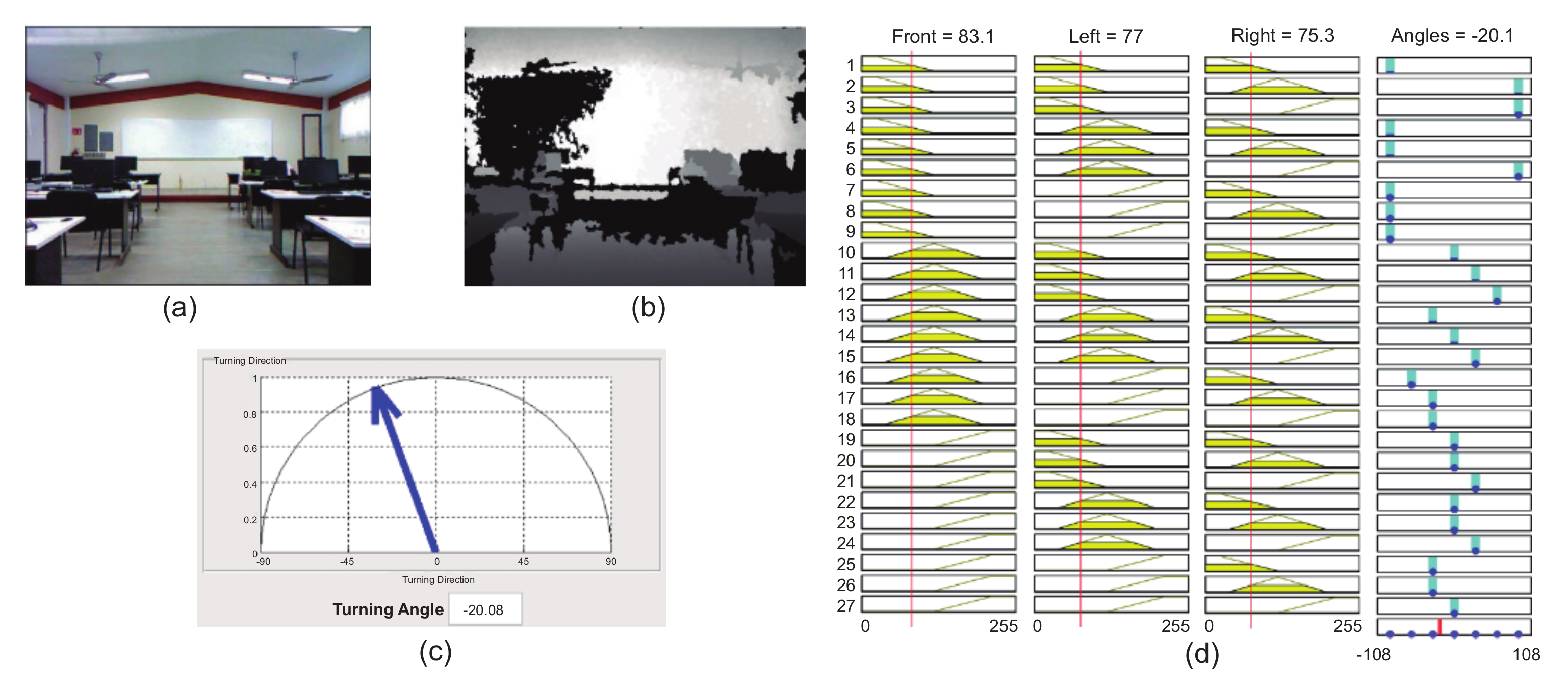
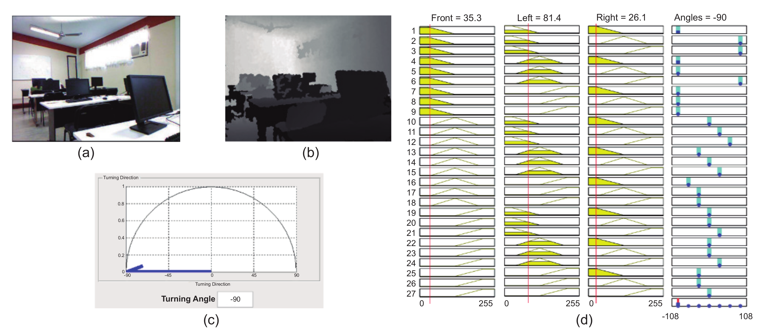
Module 4: Fuzzy logic system. This module implements a fuzzy control for the reactive navigation of the mobile platform (see Figure 6d). The used tool for this development was Matlab’s Fuzzy Logic Toolbox. The fuzzy inference system receives the average depth values obtained from each sub-image as inputs. It provides an output variable in sexagesimal degrees between −90° and 90°, representing the turning angle. A Sugeno inference system is used because it is computationally effective by generating numeric outputs and not requiring a defuzzification process. Sugeno systems work with adaptive and optimization techniques, and these implemented in navigation guarantee continuity in the output surface [30].

The depth variables obtained by each sub-image (Left, Center, and Right) are inputs. Each has three linguistic values: Near, representing the depth of the close objects, Medium, considering the depth of those objects located neither so far nor so near, and Far, to indicate distant objects (see Figure 6). Trapezoidal membership functions are used for the linguistic values Near and Far, and a Triangular one is used for Medium. These kinds of membership functions do not represent complex operations, as in the case of the Gaussian or the generalized bell-shaped functions [31].

The output variable Angle is divided into seven linguistic values to represent how pronounced the navigation turn will be. The function for the linguistic output variable is defined by Equation (4), where $V_i$ is the output variable for each linguistic value i; $A_i,B_i,C_i$, and $D_i$ are constant values for each linguistic value i; $x,y$, and z are the input variables:

$$V_i=A_{i}x+B_{i}y+C_{i}z+D_i$$

(4)

A zero-order Sugeno system was used [31] to prevent a complex behavior. Thus, the function for each linguistic variable is defined just in terms of a constant $D_i$. As described in [28], for each linguistic value, different functions were defined as follows:

• $D1=90$ for Very Positive,
• $D2=60$ for Positive,
• $D3=30$ for Little Positive,
• $D4=0$ for Zero,
• $D5=-30$ for Little Negative,
• $D6=-60$ for Negative, and
• $D7=-90$ for Very Negative.

The number of permutations in the linguistic values (Near, Medium, and Far) and the respective input variables (Left, Front, and Right) produce the set of fuzzy rules, which is defined and developed to obtain the output value corresponding to the turn in the mobile platform. The fuzzy control uses 27 rules, divided into four groups, depending on a common goal: rules for performing pronounced turns, rules for predicting collisions, rules for straight-line movements, and rules for basic turns. The set of rules is described as: If x is A, then y is B.

These rules try to emulate the human reaction during navigation since they generate gradual reactions going from performing almost no turn to abrupt moves, either to avoid unexpected collisions or on the move. The set of rules has the primary goal of executing soft turns that guarantee the mobile platform’s integrity, which is a fundamental condition in wheelchair navigation, to protect the person using it.

3.2. Case II: Mobile Robot and Neural Networks

The second case is a self-navigating robot, which uses data obtained from ultrasonic sensors and artificial neural networks to decide where to move in an uncontrolled environment: to the right, left, forward, backward, and, under critical conditions, stop. This information allows for smooth turns applying multilayer neural network architecture with supervised learning algorithms. The mobile robot decides to avoid fixed and mobile obstacles, providing security and movement in uncontrolled environments.

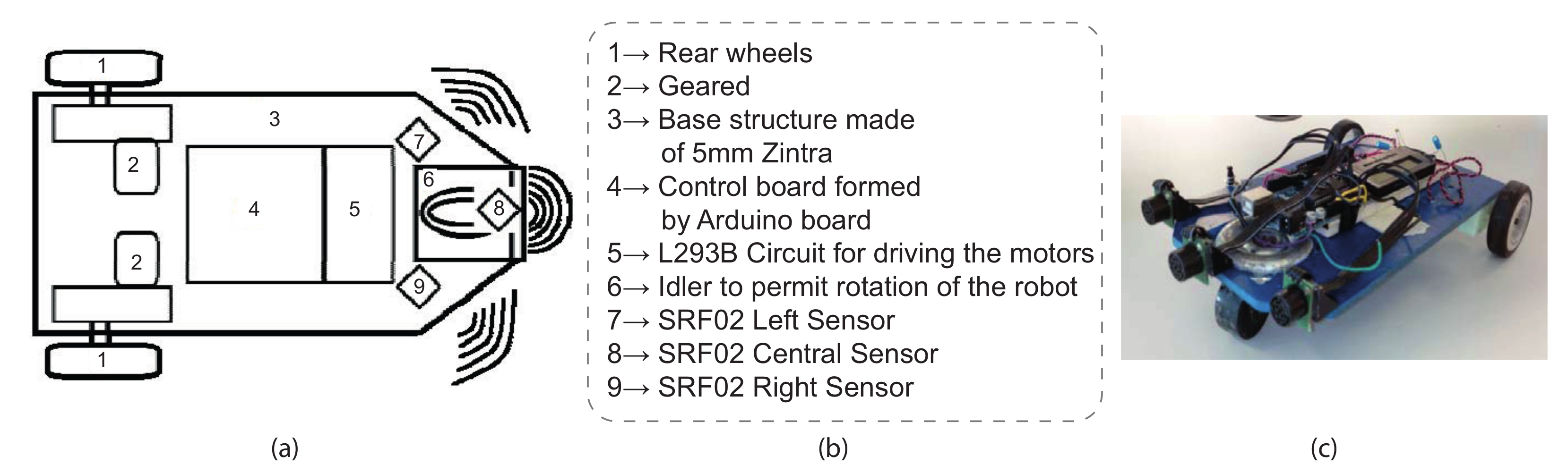
Mobile robot construction. In this case, the mobile robot algorithm applies a multilayer neural network (MLP) utilizing backpropagation. The mobile robot structure was designed to be easily modified and adaptable. Its physical appearance was evaluated to be simple with reduced size, considering previous mechanical structures of robots. Figure 7a presents the top view of the mechanical structure of the mobile robot. The localization of each device applied for its movement is also shown there. A list of each device is shown in Figure 7b, and the prototype picture is presented in Figure 7c.

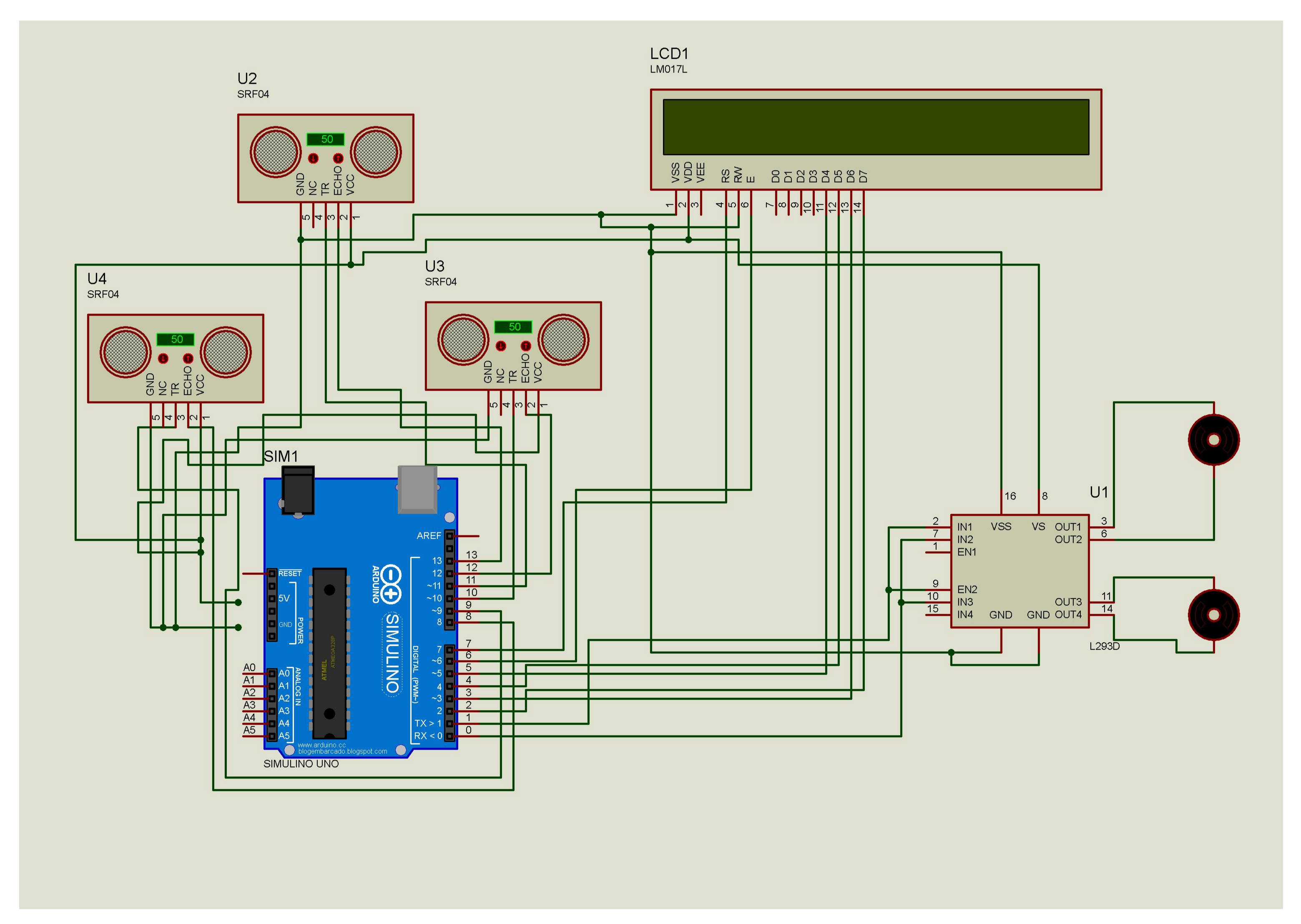
The design of the electronic connection diagram implemented in the mobile robot is shown in Figure 8, where the microcontroller, SRF02 ultrasonic sensor, $B{02}_1$-180 geared motors, and an LCD screen that displays the motors and sensor status are presented.

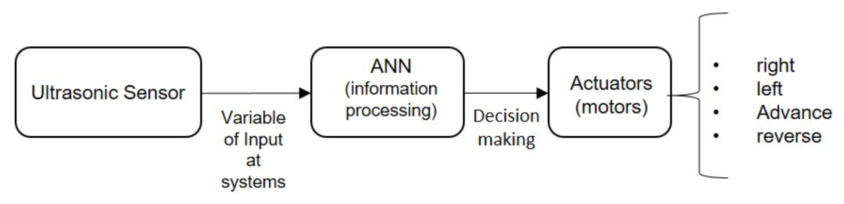
In Figure 9, the block diagram of the system operation is shown, where the system makes a decision after processing the signal from the ultrasonic sensors.

The sensors described in the first block of Figure 9 are read by means of the following code:   

Code 1: Ultrasonic sensor reading stage.

1 // Function analog sensor reading
2void read_analog ()
3 {
4     mq7_i=analogRead(A0);
5     mq4_i=analogRead(A1);
6     mq7_d=analogRead(A2);
7     mq4_d=analogRead(A3);
8     mq4_i=(mq4_i*9.481)+300;
9     mq7_i=(mq7_i*1.935)+20;
10    mq4_d=(mq4_d*9.481)+300;
11    mq7_d=(mq7_d*1.935)+20;
12 }

ANN Design to make decisions. Several applications to avoid collision of mobile robots while controlling their movements and generating a path have been developed, showing a pattern classification problem. Networks such as single perceptron, multilayer perceptron, radial basis networks, and probabilistic neural networks (PNNs), among others, have been popularly used. In this case, a multilayer perceptron (MLP) is chosen because of its general characteristics. In addition, it is an architecture that is relatively simple to implement in a robot. 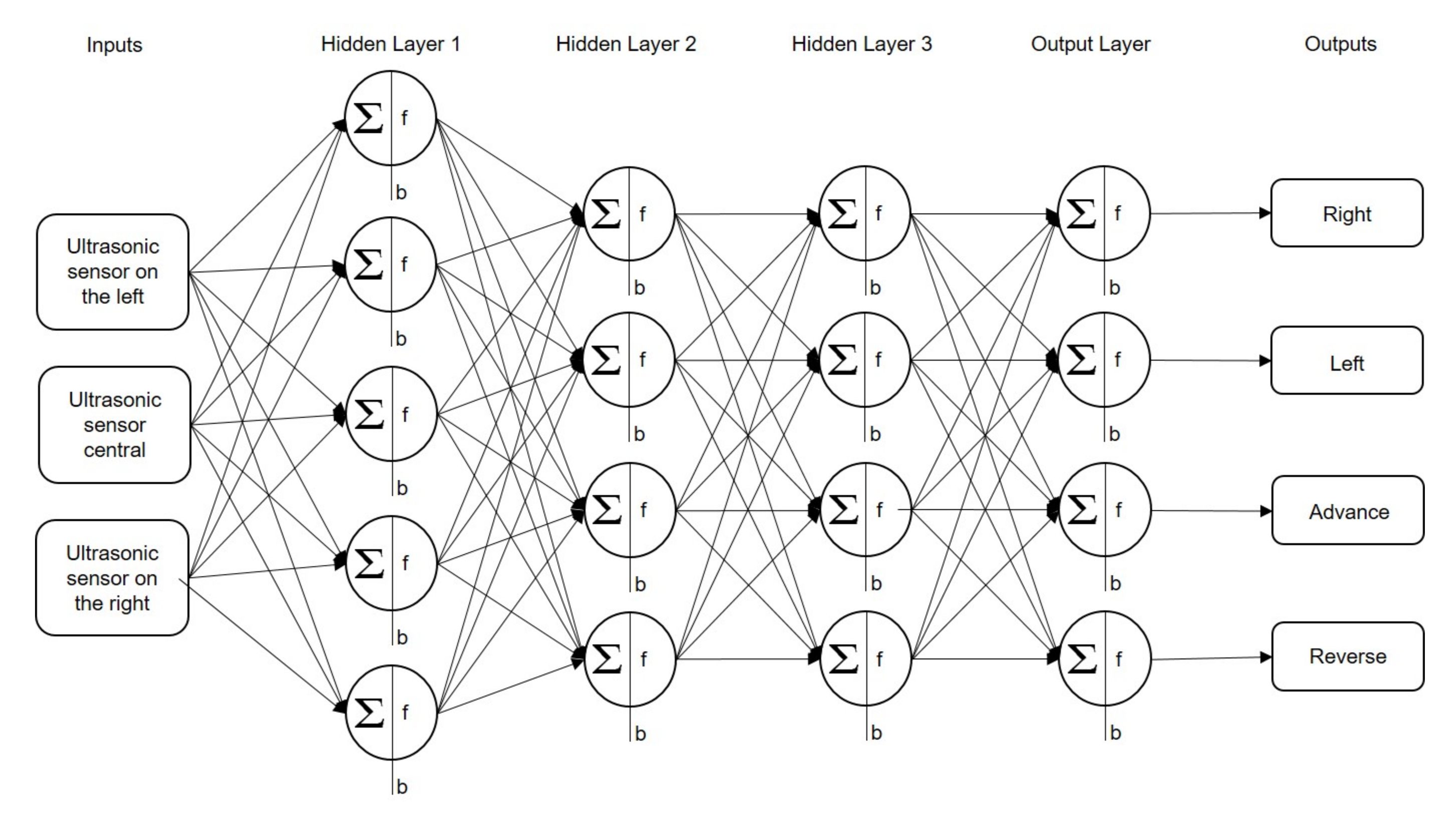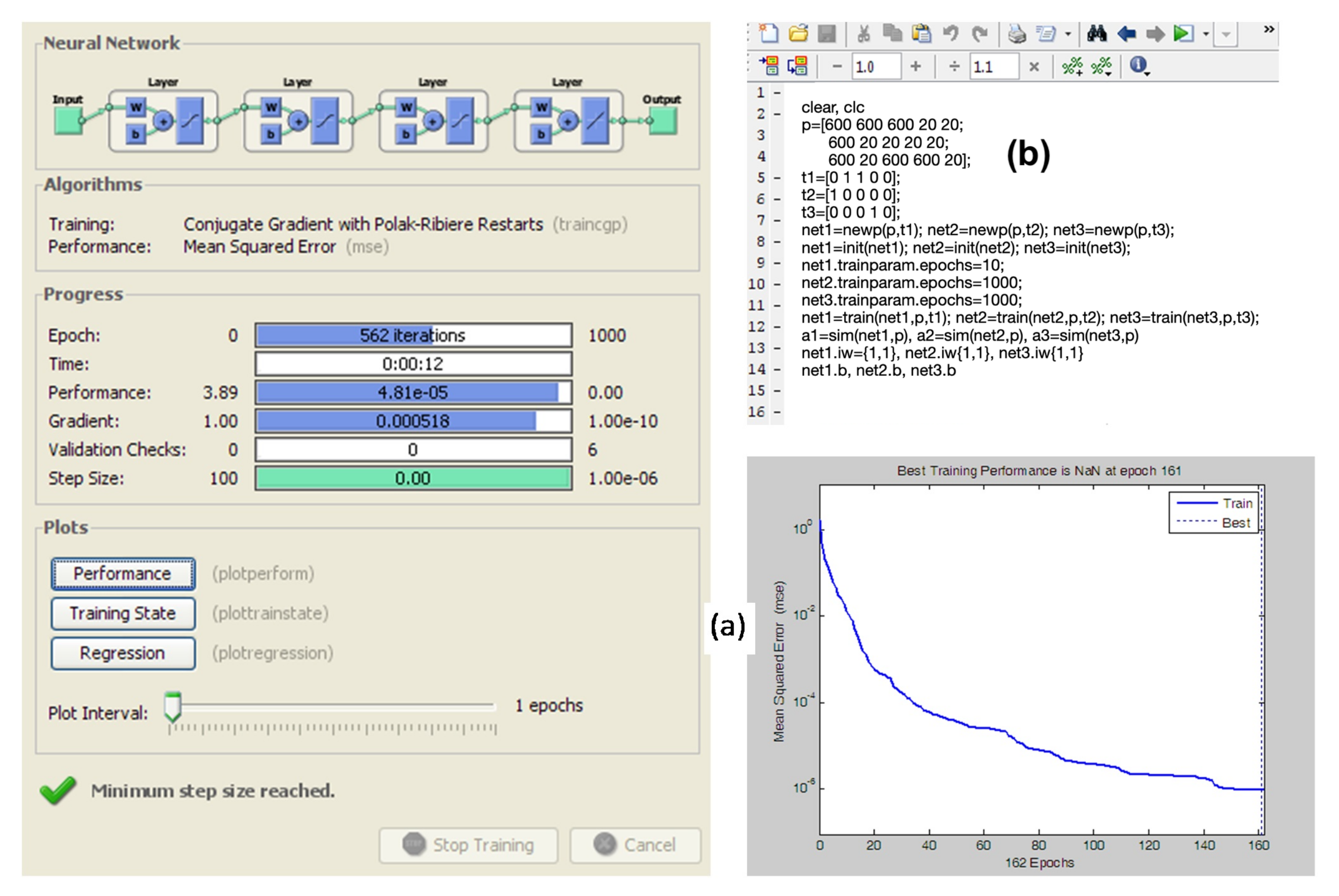Figure 10 presents the neural network structure. It consists of three input vectors and an output vector with four elements each; then, a 4-layer configuration was made [5, 4, 4, 4], in the first hidden layer using the “tansig” activation function, and a “logsig” function in the second and third hidden layer was used. The activation function applied in the output layer was the “logsig”.

Inside the robot, on the left, center, and right, ultrasonic sensors were placed, operating as the network’s inputs. These sensors are activated depending on the proximity of the obstacle in the path. The network’s output depends on these sensors that allow the proper position and hence obstacle avoidance. Decimal numbers will be the output network in the range [0 1]. After that, a comparison function in Arduino will be executed to establish the value of the output greater than 1 and the other two in 0.

Equation (5) represents the mathematical behavior of the neural network developed and implemented in the embedded system for decision-making of the mobile robot:

$$\begin{array}{c}\hfill Advance=(-0.2038\ast s40)+(-0.7043\ast s41)+\\ \hfill (0.5507\ast s42)+(0.9462\ast s43)+\\ \hfill (0.5487\ast s44)+(-0.8956\ast s45)+\\ \hfill (0.0640\ast s46)+(-0.1733\ast s47)+\\ \hfill (0.1475\ast s48)+\left(0.5903\right)\\ \hfill Reverse=(-0.2303\ast s40)+(-0.9128\ast s41)+\\ \hfill (-0.5520\ast s42)+(-0.9457\ast s43)+\\ \hfill (0.5468\ast s44)+(0.8954\ast s45)+\\ \hfill (-0.2537\ast s46)+(0.8212\ast s47+\\ \hfill (-0.3697\ast s48)+\left(0.7083\right)\\ \hfill Right=(0.2687\ast s40)+(-0.5057\ast s41)+\\ \hfill (-0.0005\ast s42)+(-0.0016\ast s43)+\\ \hfill (0.5008\ast s44)+(0.0002\ast s45)+\\ \hfill (-0.2192\ast s46)+(-0.1973\ast s47)+\\ \hfill (-0.5429\ast s48)+\left(0.2895\right)\\ \hfill Left=(0.8263\ast s40)+(-1.1277\ast s41)+\\ \hfill (0.0032\ast s42)+(0.0022\ast s43)+\\ \hfill (-0.5025\ast s44)+(-0.0013\ast s45)+\\ \hfill (-0.9629\ast s46)+(-0.9097\ast s47)+\\ \hfill (-0.7474\ast s48)+(-0.6503)\end{array}$$

(5)

4. Results and Comparisons

In the following, the results and comparisons of the two cases presented before are shown and explained. Moreover, how mobile robots reacted to obstacle presence is described.

4.1. Case I: Mobile Robot and Fuzzy Logic

The tests of the reactive fuzzy navigation system were carried out in a computing laboratory. The Kinect sensor’s height is 0.78 m with a vertical tilt of 0 degrees, and it is located on the mobile platform Era-Mobi. The fuzzy control system works on the depth images, using the RGB images as a human visual reference. One thousand experiments were run to compute execution times for the analyzed system, where the image capture time, the running time for each of the four stages, and the total time are measured.

The computing of the turning angle by using fuzzy control requires a higher consumption of computational resources. The morphological reconstruction process expends the least time with 4.8 ms, where the fuzzy reactive navigation system performs its operations in a range between 38.9 ms and 43.5 ms. The Kinect sensor at 30 Hz requires an approximate time of 33.33 ms. A client system was programmed. In addition, a client/server player application is implemented on the robot’s onboard computer to communicate and execute the mobile robot’s turning angle. In the performed tests, the system made accurate decision choices regarding the turning to avoid obstacles in 85.7% of the attempts.

Figure 11 and Figure 12 show the system performance in the test environment with no object movement and moderate lighting. Parts (a) and (b) show the RGB image and its corresponding depth image, respectively. Part (c) shows the output of the fuzzy system, which processes and identifies depth in each division of the image, gives linguistic values, and produces the turning angle in degrees (see part (d)), respectively. It is shown that the system tries to follow the path with the lowest probability of collision, reporting stability while going through spaces with known information. Depending on the amount of known data, the system infers if it must either ignore them or consider them for computing the average depth for each sub-image. On the one hand, Figure 12 presents a situation where there are many objects that are obstacles, and the fuzzy control indicates to turn left, which has a value of −90.00°. On the other hand, for Figure 11, the system determines a soft turn of −20.08°. It is possible to examine the behavior for the output variable (turning angle) using the combination of the inputs that vary as a product of possible changes in the environment (obstacles or noise) and a constant input.

Part (d) is the inputs of the turnAngle function, which produces an angle for avoiding obstacles. Algorithm 1 presents a pseudo code, where $V_i$ are computed from $D_i$, and the rule set is described in

Table 1. Fuzzy Inference Matrix.

Ruleset	No.	If			Then
Sharp Turns	1	Near	Near	Near	Very Negative
	2	Near	Near	Medium	Very Positive
	3	Near	Near	Far	Very Positive
	4	Medium	Near	Near	Very Negative
	5	Medium	Near	Medium	Very Negative
	6	Medium	Near	Far	Very Positive
	7	Far	Near	Near	Very Negative
	8	Far	Near	Medium	Very Negative
	9	Far	Near	Far	VeryNegative
Predictive Rules	10	Near	Medium	Medium	Little Positive
	11	Medium	Medium	Near	Little Negative
	12	Medium	Medium	Far	Little Positive
	13	Far	Medium	Medium	Little Negative
	14	Far	Medium	Far	Little Negative
	15	Near	Far	Far	Little Positive
	16	Medium	Far	Far	Little Positive
	17	Far	Far	Near	Little Negative
	18	Far	Far	Medium	LittleNegative
Straight Line	19	Near	Medium	Near	Zero
	20	Medium	Medium	Medium	Zero
	21	Near	Far	Near	Zero
	22	Near	Far	Medium	Zero
	23	Medium	Far	Near	Zero
	24	Medium	Far	Medium	Zero
	25	Far	Far	Far	Zero
Smooth Turns	26	Near	Medium	Far	Positive
	27	Far	Medium	Near	Negative

.

Algorithm 1: Main fuzzy control function.

Function $turnAngle$ Angle in sexagesimal degrees

Input:$Left\left(x\right)$, $Front\left(y\right)$ and $Right\left(z\right)$

Output:$turnAngle(x,y,z),$

$fuzzification1\left(x\right),$$fuzzification2\left(y\right)$ and

$fuzzification3\left(z\right)$

for each member i of the $Ruleset$ do

$W_i=fuzzyOperation1\mathrm{AND}fuzzyOperation2$

$V_i=D_i$

end for

$turnAngle=\frac{{\sum }_{i=1}^N{W}_i\ast V_i}{{\sum }_{i=1}^N{W}_i}$

The Sugeno fuzzy inference system is chosen instead of the Mamdani system, since it is not necessary to generate information for the human being, but for motor control. Additionally, this allows a lower computational load because the Sugeno approach does not require any fuzzification module.

The three aspects of analysis considered were: (1) image format, (2) number of bits for representing depth, and (3) membership function. The first aspect is related to image formats that Kinect can process: point cloud and depth images. We generate the same image using point cloud images and depth images, and we observe that point clouds need significantly more disk storage space than depth images (on average, about 1 MB per capture). The processing time between both formats may differ depending on the hardware and software available. However, the point clouds suggest an average 30-s processing time per capture, based on experimental data shown in [13,14], ranging from 13.6 s to 41.1 s. We compare resource consumption regarding space among the algorithms mostly used by point clouds, when they are coupled to a reactive architecture. The comparison shows that the response time does not present any improvement related to depth images. The second aspect, the 8-bit versus 16-bit values, was analyzed, and, due to the definition of three linguistic variables, the division of the different ranges does not cause any loss in the evaluations. Consequently, there is a better computational time, which is generated by using smaller data bit size. The third aspect considers the definition of the ranges for the type of membership function, where the extremes of the value close to 0 and 255 are defined in such a way that the function does not allow the membership value to decrease, resulting in soft turns or straight-line navigation (in case the objects in the three directions are too far away). For external values, the trapezoidal membership function is used. For intermediate values, the triangular function is implemented since the turns should not be so pronounced, and the system must have a midpoint where it allows a constant output. The trapezoidal and triangular functions do not require complex operations, as compared to the Gaussian function, which is expressed using exponentiation and potentiation operations. The proposed architecture focuses on the least amount of calculations and preserves enough information for decision-making. Membership degree for each value x is defined by evaluating it on its corresponding membership function (fuzzification). Figure 13 shows an example of fuzzification where x = 1.6 with triangular function, obtaining a membership degree of $\mu$ = 0.4.

4.2. Case II: Mobile Robot and Neural Networks

The output vector comprises three elements that correspond to each of the basic activities that control the mobile robot. Their element values are coded so that the respective movement to run is 1, and the other three are equal to 0. Thus, the neural network will produce the output vector (1,0,0,0) if the control of the action is to turn right, a vector (0,1,0,0) if it is turn left, a (0,0,1, 0) vector if the action is to advance, and, finally, a (0,0,0,1) vector if it is back. The designed decision-making algorithm is shown in Figure 14.

The neural algorithm was developed and implemented in the mobile robot as an integrated system; the coding was carried out in Matlab. The architecture of the neural network and the learning algorithms’ design are monitored and disconnected in the Matlab software, where the values of synaptic weights and bias extract the link, respectively.

Figure 15a shows the training characteristics concerning the behavior of the mid-squared error of the neural network in the backpropagation training. Matlab shows satisfactory results observed in training, where Figure 15b shows the script for system simulation and implementation.

The programming of the neural network designed for the mobile robot as an integrated system was based on (1) synaptic weights of the hidden layers, (2) synaptic weights of the output layer, (3) bias or weights of each layer, and (4) knowledge of the activation functions that are used in each of the layers. In the first hidden layer, tansig is used and, in the remaining layers, logsig is used.

The synaptic weight matrices of the architecture of Figure 10, where W1, with five rows and three columns, stores the weights that connect the input layer with the hidden layer. The input variables are obtained from vector X. In addition, the weights connecting the hidden layer with the next layer are stored in matrix W2, which is composed of four rows and five columns. In the case of the weights that connect layers, they are stored in matrix W3, which consists of four rows and four columns. Finally, as with the last hidden layer and the layer’s output, the data are stored in matrix W4, which has four rows and four columns. It is important to note that the bias corresponding to each layer is stored in a vector, to have four vectors, which are b. After processing the information, the output obtained from this network decides the action to be taken. Therefore, this information is used so that the robot can avoid obstacles found in the environment.

Physical implementation and analysis. The dimensions of the robot in Figure 7c are 26-cm length, 12-cm high, 24-cm separation between wheels, and an average speed of 10 cm/s traveling in a straight line. The wheels were covered with non-slip material to improve the performance on smooth surfaces. The sensors work correctly because the sensors for this type of object must be made of relatively dense materials. The aim is that the reflected ultrasonic signal is properly generated and then detected by the transducer.

The algorithm used for robot learning and navigation was implemented in Matlab language and can easily be extended to include new restrictions and actions in the environment. The robot’s adaptability was verified by the interaction of the robot with a group of people in an open exhibition space. People played the role of dynamic obstacles, i.e., they used their feet to block the mobile robot’s movement, even if they had another mobile robot.

Table 2. Simulation of neural architectures for mobile robots.

Training Type	Neural Architecture	Epochs	Training Time	Performance	Training: R	Total Response Time (s)
Trainbr	3-5-4	301	83.734	0.534	0.25	83.804
Trainbfg	3-5-4	100	26.273	8.01 × 10${}^{-06}$	0.99999	26.343
Trainscg	3-5-4	225	49.822	9.98 × 10${}^{-06}$	0.99999	49.892
Traincgb	3-5-4	100	23.761	8.87 × 10${}^{-06}$	0.99999	23.832
Traincgf	3-5-4	144	36.303	E1.00 × 10${}^{-05}$	0.99999	36.373
Traincgp	3-5-4	80	18.6305	9.97 × 10${}^{-06}$	0.99999	18.7005
Trainbr	3-5-4	365	10.5156	5.33 × 10${}^{-06}$	0.25	10.5856
Traincgb	1-4-5-4	125	1.6563	9.89 × 10${}^{-06}$	0.99999	1.7263
Trainscg	7-3-4	100	2.5469	9.37 × 10${}^{-06}$	0.99999	2.6169
Trainbfg	3-5-6-4	83	38.7656	9.76 × 10${}^{-06}$	0.99999	38.8356
Trainbr	2-5-6-8-9-4	15	11.8906	5.37 × 10${}^{-06}$	0.24992	11.9606
Traincgp	2-5-6-8-9-4	284	128.9219	2.88 × 10${}^{-05}$	0.99997	128.9919
Traincgp	5-4-4-4	116	7.30	9.40 × 10${}^{-06}$	0.99999	7.37

shows results obtained by different neural architectures and backpropagation learning algorithms, implemented for decision-making in the mobile robot in the presence of obstacles in front of the used ultrasonic sensors (the sensors’ average response time was 65 ms). If we analyze the architectures presented in Table 2, we can observe short and long architectures with fast response times and different processing accuracies. The first case is the 3-5-4 architecture, which has a response time of 10.5856 s with a 25% accuracy; a second case is the 1-4-5-4 architecture, with a response time of 1.7263 s and 99.99% accuracy. The implementation of the architecture in the embedded system for field tests will depend directly on this analysis for decision-making in the mobile robot.

Table 3. Average execution times (ms).

Equipment	Capture	Decision-Making	Fuzzy Logic	ANN	Total Response Time
Laptop Windows 7, Core i7, 2.3 GHz, 8 GB RAM	10.4	15.6	X		38.9
PC Windows XP, Core Duo, 3.16 GHz, 3 GB RAM	6.4	18.9	X		43.5
PC Windows 10, Intel(R) Core(TM), 2.70 GHz, 16 GB RAM	65 ms	10.5156		X	10.5856
Embedded System (Arduino R3), ARM Microprocessor, 33 MHz	65 ms	10.5156		X	17.2536

shows the response times of the fuzzy and neural systems for information processing and decision-making. We observe that implementing neural networks would be appropriate for their fast response time. Still, we would be probably sacrificing accuracy in the robot movements, as opposed to what would happen with the improved accuracy of fuzzy logic. Hence, the decision on which one to choose will ultimately depend on the end-user application.

5. Discussion

We identified strengths and challenges of reactive Obstacle–Avoidance systems based on approaches of an ANN-BP architecture and FIS rules. We show the comparisons in

Table 4. Environmental input data.

Navigation Technique	Input Signals	Field of View (Measurement Angle)	Measuring Distance	Response Time (ms)	Sensor
ANN-BP architecture	Analog data	Horizontal field of view: 15 degrees	From 0.10 m to 3 m	10.6	Ultrasonic
FIS with Kinect	Digital image	Horizontal field of view: 57 degrees; vertical 43.5 degrees	From 0.8 m to 4 m	38.9	Kinect: only RGB-D

,

Table 5. Environmental operating conditions.

Navigation Technique	Performance Measure	Ambient	Static Obstacle	Dynamic Obstacles	Real-Time Results
ANN-BP architecture	Accuracy	Real-world dynamic in 2D	Yes	Yes	Yes
FIS with Kinect	Turn smoothness accuracy	Real-world dynamic in 3D	Yes	Yes	Yes

and

Table 6. Comparison of reactive Obstacle–Avoidance systems.

Navigation Technique	Detected Objects	Surface Type	Affected by	Strengths	Challenges
ANN-BP architecture	Transparent, liquids, and irregular shaped objects	Rough, smooth, and bright	Temperature, environments with pressure present, and they do not detect foam objects	(i) Supervised learning, (ii) Scalable neural architecture, (iii) Neural architecture with implementation in embedded systems for real-time experiments	(i) Convergence of the ANN depends on the number of neurons in the architecture, (ii) Using the BP training algorithm provides very good results, (iii) The number of interconnections in the neural architecture increases proportionally with the number of neurons used in the architecture, (iv) Difficult to acquire its required large data-set of the environment during training to achieve best results.
FIS with Kinect	Triangular, rectangular, square, circular objects, which differ by depth	Rough and smooth	Objects and surfaces made of transparent, reflective, and absorptive materials	(i) Smooth movements, (ii) Multiple objects detection, (iii) Robust to rotation and translation, (iv) Partially robust to scaling and occlusion, (v) Robust to environmental noises, (vi) Object recognition with digital signatures	(i) Calibration of rules, (ii) Environment calibration, (iii) Increase databases for object detection, (iv) Sensor data fusion (RGB and depth sensors) to increase distance detection

. We highlight in these tables differences regarding the environmental input data collected by the robots in the real world, the environmental operating conditions, and a comparison of the conditions considered for obstacle avoidance. Therefore, in the analysis, we consider aspects such as: sensor response, field of vision, distance measurement, type of objects identified, type of surface, real experimental environment, effects or noise over the sensors, dynamics of the real environments, limitations of the mobile robots that affect the reliability, and efficiency of approaches to work well in real-world deployments. In addition, we present a summary of the strengths and challenges of the approaches considered. The strengths define the main contributions of each approach to avoid obstacles. The challenges describe the problems that must be solved to measure how successful or efficient these approaches would be when implemented in the real world where real conditions exist. An important remark is that we were able to identify that, to the best of our knowledge, most of the approaches published elsewhere were implemented only in a simulated environment, such as [15,16].

6. Conclusions

Wheeled mobile robots have allowed human beings to perform activities in challenging-access environments, such as radioactive zones, space, explosives, etc. In turn, designing, modeling, and testing mobile robots require techniques to enable prototypes to achieve a proposed objective in the environment. Whether the models have different characteristics must be considered, such as the robot’s physical structure, movement restrictions, components, etc.

In this paper, two different cases of mobile robots using artificial intelligence were presented to avoid obstacles. The first applied fuzzy logic rules with depth images as an input pattern, obtaining a turning angle as output. The second case involved a multilayer perceptron network that uses ultrasonic sensor signals as input vectors to generate four possible outputs. As shown in the results of both cases, the performance achieved by mobile robots is optimal, completing their main objective of avoiding a collision.

What can be learned from the analysis of these two very different implementations of intelligent reactive Obstacle–Avoidance systems for mobile robots is that the use of artificial intelligence is of benefit to facilitate the interaction of a robot either in a static or a dynamic environment. Although a robot designed based on a predefined navigation map is expected to behave adequately using this map, it is frequently not the case that its behavior is good in the presence of dynamic environments. This subtle difference, mostly due to the use of artificial intelligence, which allows the robot to have a reactive behavior, must be emphasized since this makes a difference between designing a mobile robot that is only prepared for laboratory-conditions and designing it for working in real-world environments, where the interaction with humans and other mobile robots is definitely not part of a static environment.

As a remark, even with different artificial intelligence techniques, fuzzy logic, and artificial neural networks, we can appreciate that both are good options for mobile robot applications. Furthermore, as mentioned previously, many hybrid systems have been proposed in the literature, which provides several alternatives for implementing reactive mobile robots using artificial intelligence.

Another thing we can learn is that it is certainly important that the choice of a particular technique will mostly depend on the kind of application since the number of computational resources, such as available memory, computing power, sensors, etc., will determine the kind of technology that is more suitable for the particular implementation. Given these limitations, it is not always feasible to implement these systems using a certain technique. Another aspect, just as important and quite related to the available hardware resources, is how fast the response needs to be since, for example, a mobile robot in an industrial environment has quite different requirements in terms of response time compared to those of an autonomous vehicle. By analyzing these requirements and restrictions, the most suitable technique for the implementation of such a mobile robot is more likely to be properly determined.

As we have explained, although the two analyzed cases are based on heuristic approaches, both differ in certain aspects. While, in the former case, the use of fuzzy logic provides a more reliable behavior while processing uncertain data, the need for an expert in the field, capable of properly defining the rules the system will use to make a decision, might represent a clear disadvantage in terms of ease of implementation. However, once the rules are defined, this knowledge helps the system make fast and accurate decisions; in addition, the fact that these systems need no training for working represents an advantage in certain contexts. On the other hand, in the analyzed case using artificial neural networks, the need for training might be seen as a disadvantage since this training might take a long time and several resources, limiting the kind of devices where this kind of solution can be satisfactorily implemented; nonetheless, the training of the system, in certain problems, can be made offline, which serves to avoid the problem of limited resources; in addition, once trained, a system based on artificial neural networks is capable of making fast and reliable decisions as well.

The response time of systems is affected by how fast they generate the inference. In addition, the type of information processed influences their precision. In addition, the processing time is highly coupled to how sensors react throughout the inferences system’s signals. For instance, the mobile robots applying MLP presented in this paper, both physically implemented, can present zigzag movements according to the neural architecture. Nevertheless, the fuzzy control carries out a slow response but smooth movements. In the case of the application of neural networks, the physically employed system’s response time is 17 s between one decision-making and another (data obtained in a field test). In contrast, the fuzzy control decision time is 38.9 s.

One aspect that cannot be ignored is the possibility of using fusion techniques for integrating several different sensors for composing a more sophisticated solution. This represents the inclusion of more than one type of input vector for mixing these sensors’ information. In addition, the possibility of hybridizing techniques like these is attractive for future implementations; for example, by learning the fuzzy rules using an artificial neural network, instead of depending on expert knowledge, such as in the case of the adaptive neuro-fuzzy inference system (ANFIS) [32].

Many works can still be developed in the area of mobile robots. The used approaches will depend on robots’ application, environment, and their main purpose or function. Currently, for example, mobile applications for hospitals are being used to guide and/or support the transport of hospital equipment for better delivery and reception times in necessary areas.