Featured Application
The results of the research as well as the technical aspects of the proposed method could be used for support managers’ decisions in retail stores related to allocation products on shelves.
Abstract
This paper discusses the problem of retailers’ profit maximization regarding displaying products on the planogram shelves, which may have different dimensions in each store but allocate the same product sets. We develop a mathematical model and a genetic algorithm for solving the shelf space allocation problem with the criteria of retailers’ profit maximization. The implemented program executes in a reasonable time. The quality of the genetic algorithm has been evaluated using the CPLEX solver. We determine four groups of constraints for the products that should be allocated on a shelf: shelf constraints, shelf type constraints, product constraints, and virtual segment constraints. The validity of the developed genetic algorithm has been checked on 25 retailing test cases. Computational results prove that the proposed approach allows for obtaining efficient results in short running time, and the developed complex shelf space allocation model, which considers multiple attributes of a shelf, segment, and product, as well as product capping and nesting allocation rule, is of high practical relevance. The proposed approach allows retailers to receive higher store profits with regard to the actual merchandising rules.
1. Introduction
Retailing is a very competitive industry highly dependent on profit [1]. Efficient shelf space allocation is critical in gaining a competitive advantage [2]. The shelf on which products are being displayed is one of the most critical resources in the retail environment as retailers can increase their profit and simultaneously decrease cost by proper management of shelf space and product display [3]. Customers are also influenced by floor and space planning or assortment planning [4]. Retailers work with the goal of profit and sales maximization, allocating a limited amount of shelf space in a practicable way [5].
Retailers use a planogram to plan product allocation on shelves, which is a diagram or model that indicates the placement of offered products on shelves [6,7,8,9]. Of course, maximization of sales is dependent not only on efficient category planning but also on marketing and merchandising of products. Parameters such as unusual product shapes, colors, promotional additions, etc., may disturb the perception of shelves and product allocation. Still, the retailer’s regular work lies in consecutive decisions regarding the following problems: to determine the assortment size, allocate the assortment product items to the shelves, specify prices and discounts, and manage in-store shelf replenishment. Retail shelf management involves quickly and cost-effectively matching retail operations with customer demand [10].
Shelf space seems to be a scarce and expensive resource in the retail industry as a large number of products compete for limited display space. Therefore, shelf-space allocation is frequently implemented in shops to increase product sales and profits [11]. The problem of optimally allocating products presentation spaces to maximize revenues is of great importance to retailers [12].
Shelf space planning designates the position of products on a shelf and the number of facings of each selected product under limited shelf size constraints. Actual product sales may depend on the product’s quantity and location on the shelf [13].
The shelf space allocation problem (SSAP) is a decision problem where the goal is to achieve the best possible result under various operational constraints in a retail store. It is regarded as an extension of the knapsack problem [14]. The SSAP aims to determine the optimal mix of product displays to maximize profitability. Decisions on the right product at the right location with the proper space allocation are necessary when shelf space is limited [15].
The main SSAP literature research gaps are:
- considering only length limit as shelf capacity parameter;
- considering only basic constraints;
- omitting capping and nesting allocation parameters in all models;
- not investigating the shelf segments of flexible size.
Most of the SSAP models in literature treat available shelf space one-dimensionally, estimating it in shelf length or in volume [2,4,5,16,17,18,19,20,21,22]. Shelf capacity is usually defined as a single, real value. Another key point is that the SSAP literature omits the possibility of product capping (placing the product on the top of the product with rotation of the upper product to push in more products on the shelf space even if the product on its main orientation does not fit) and nesting (placing the product into the product as a bucket). There is no model that considers such decisions.
Motivated by those findings, we focused on the SSAP to deal with how to efficiently allocate shelf space to each product to maximize the total profit volume. The aim of this paper is to develop a mathematical model and a genetic algorithm for improving the shelf space allocation with the criteria of retailers’ profit maximization.
The main contribution is related to the following issues. The majority of SSAP models use a basic set of constraints such as capacity, face size, lower and upper bound, allocation, and profit. However, in retail real-life, there are significantly more constraints. Our research focuses on cappings and nestings and enhances the main model with these parameters. In this research, in addition to the basic set of constraints, we investigated shelf constraints (shelf weight, height, length limits), shelf type (whether a shelf is suitable for such type of a product and whether a product is allowed to be placed on the specific shelf), product constraints (as well as facings, capping and nesting are taken into account, and product size and weight parameters), and special segments constraints (on which part of the shelf the product must be allocated). These were grouped into four main categories.
We present the SSAP model, which takes into account the above constraints. Next, we solve it using a genetic algorithm and repeat computational experiments on relevant practical problem sizes to compare our designed solution with the CPLEX one. Our approach’s kernel may be used to automate the retailers’ complex decisions to deliver higher profits.
This paper is organized as follows. The theoretical background is given in Section 2. In the following Section 3 and Section 4, the SSAP definition and its mathematical model are presented. The genetic algorithm is given in Section 5. Further, in Section 6, the results of computational experiments are demonstrated. Section 7 highlights the discussion of findings. The article is concluded in Section 8.
2. Theoretical Background
Many types of research have focused on SSAP in the context of retailers’ profit maximization as efficient shelf-space management influence on product sales [18,23,24]. According to Baron et al. [25] and Tsao et al. [26], attention has been given to shelf space allocation models [27].
Hübner and Schaal [28,29] provided a model which combines assortment and shelf space planning decisions and considered stochastic and space-elastic demand as well as out-of-assortment and out-of-stock substitution effects.
Practical guidelines of the impact of cross-space elasticities and product substitutions on shelf space decisions are given to retailers by Schaal and Hübner [30]. Urban [16] models the demand function, including the inventory level dependent decisions, and divided the backroom and the showroom inventory. Hübner and Schaal [28] incorporated the optimization model with in-store replenishment processes. The demand increased if there was more shelf space designated for a product because of the higher visibility while replenishment was decreasing and inventory costs were also increasing.
Generating planograms is a complicated and time-consuming task due to the vast number of retail and marketing constraints, the majority of which are non-standard. The problem is already reduced to a multi-knapsack, one of which is NP-hard [4]. Commercial software uses heuristics rules to solve the SSAP to help retailers [10,13,14,16,28,29,31].
Researchers apply specialized heuristic and metaheuristic search algorithms to the SSAP to reduce the time to solve the problem [21]. Unfortunately, such algorithms do not guarantee an optimal solution globally. Heuristic solutions are also used for planogram evaluation, which involves comparing the product positioning on the planogram and the template planogram. Frontoni et al. [9] proposed a heuristic approach that finds and counts multiple instances of the same product in planogram maintenance. Borin et al. [32] introduced a model that combines shelf space allocation, assortment, and inventory processes using a heuristic solution approach based on simulated annealing. Ghazavi and Lofti [33] introduced a simulation-optimization approach for replenishment planning and shelf space allocation, taking into account customers’ shopping paths with the demand for various products. They developed a genetic algorithm and hybrid genetic algorithm with an imperialist competitive algorithm. Urban [16] generalized inventory management and SSAPs in retail management and proposed a greedy heuristic and genetic algorithm for the consolidated problem. Drèze et al. [5] developed a model to evaluate the effects of reallocating the product on the shelf and its influence on sales of individual brands within the product category.
Yang [18] used a knapsack formulation problem model and demonstrated a heuristic approach for solving some examples of the SSAP. Bai and Kendall [4] investigated automatic planogram generation using a simulated annealing-based hyper-heuristic framework and a set of low-level heuristics. They formulated a model as an extension of the multi-knapsack problem. Yang and Chen [17] proposed a non-linear integer programming model for shelf space allocation that could be used in retail. They categorized shelf space management strategies (dominance, adaptation, passiveness) based on the questionnaire approach. Reyes and Frazier [34] formulated a non-linear integer SSAP problem taking into account the dependency between profitability and customer service factors. Gajjar and Adil [22] provided retail SSAP with a linear profit function and developed heuristics to solve the model. Lim, Rodrigues, and Zhang [2] extended the basic, linear shelf space allocation model with product grouping and non-linear profit functions, developed a network-flow model and used local search with a metaheuristic to find near-optimal solutions. Hansen, Raut, and Swami [21] investigated the vertical and horizontal location effects and compared heuristics for decision models with facing-dependent demand.
A piecewise linearization method, which is used to approximate a complex, non-linear retail shelf space allocation model, has been investigated by Gajjar and Adil [20] and Irion et al. [31]. Quantitative models and software applications analysis in assortment and shelf space management planning has been shown in the research of Hübner and Kuhn [14]. Jajja [35] performed analyses using the dynamic system approach to find the optimal shelf space allocation and to evaluate different space allocation scenarios in stores. Fadılolu, Karaşan, and Pınar [36] proposed an optimization model, which produces an optimal product stock keeping unit list on the shelves, based on profitability. Lim et al. [19] provided a network flow model for SSAP and demonstrated that network-flow algorithms could find excellent results.
Elbers’ study [37] on the impact of store layout and shelf design on consumer behaviour showed that eye-level is the most profitable shelf location, lower shelves are reserved for the cheap products, higher shelves are for the expensive products, and central shelf space is intended for products perceived to be popular. The principle of interlacing the shelf space allocation with the store layout determines which product categories should be placed next to one another. A store layout must fulfil the customers’ needs by intuitive product differentiation and placing while also meeting the retailer’s goal of displaying to the customer as many products as possible and increasing sales. This is achieved by encouraging visitors to buy complementary products that are linked to the main ones.
An essential factor in shelf space allocation is the impact of spatial relationships between items on demand. When two items are placed together in a retail store, there is a cross-impact on their sales [27]. Desrochers and Nelson [38] suggested the improvement of item placement decisions through the use of consumer behavior.
3. Problem Definition
The problem concerns constructing a planogram, i.e., allocating products on shelves, where shelves are divided into virtual segments, to maximize the predicted profit from selling these products. In this research, we define the term virtual segment, which means visual shelf dividing into the parts for correct products allocation based on their types. There are no physical borders between the segments on the shelf, and the division is only virtual and used only by space planners. Clients see visual groups of product allocation, e.g., by category. Such allocation of products on the shelves helps the clients examine and compare the products along the shelves.
Each shelf is described by the shelf length , the shelf height , and the product’s weight limit . Moreover, depending on the vertical shelf position, the types of shelf can be specified and described by the binary parameters:
- the shelf is a pallet (which is located on the floor and used for big heavy products), ;
- the shelf is at eye level (used for expensive products or VIP products), ;
- the shelf is at a lower level (used, for example, to display children’s products), .
A shelf is divided into virtual segments for correct product allocation based on their position constraints. It is supposed that all virtual segments have equal width on the shelf. The width of the virtual segment is , i.e., it is possible to divide the shelf length into the number of virtual segments on this shelf without a remainder.
Depending on the horizontal position of the shelves and the customers’ traffic direction, there are several types of a virtual segment ():
- the virtual segment is used for local products, ;
- the virtual segment is used for convenience products, ;
- the virtual segment is situated in the central part of the shelf;
- the virtual segment is situated near the first aisle;
- the virtual segment is situated near the last aisle.
The shelf index describes virtual segments , and the index of the virtual segment on this shelf is ), consequently, i.e., local and virtual convenience segments are defined by the index of row and index of the column on a planogram.
Each product is characterized by its width , height , and weight . The supply limit of the product restricts the maximum availability of the product, which can be allocated. The quality of allocation is evaluated based on the unit profit of the product , i.e., .
Figure 1 and Figure 2 present the general idea behind cappings and nestings allocation methods. Products can be capped (i.e., placed one on the top of the other in another rotated orientation, Figure 1) or nested (i.e., placed one inside the other, Figure 2) or neither. Thus, denotes the nesting coefficient for the product, which indicates additional height for one nested item (e.g., the extra bucket height if buckets are placed inside each other). For products that cannot be nested .
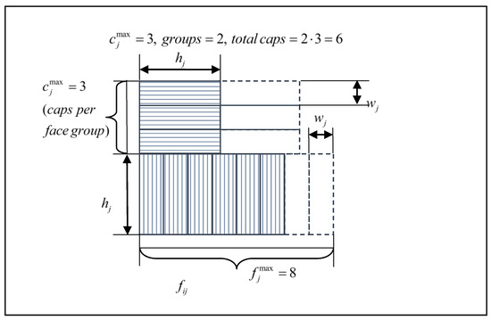
Figure 1.
Cappings allocation example for two groups and three cappings per group.
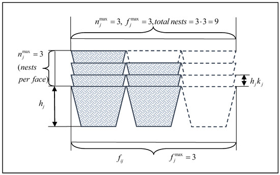
Figure 2.
Nestings allocation for 3 facings and 3 nestings per facing.
The retailer gives the minimum and maximum quantities of facings of the products that should be allocated on the shelves. They provide the best product visibility on the shelf. Moreover, the minimum and maximum side cappings per position may be restricted for each product. is the maximum number of cappings that can be physically placed above the facings row without destroying them due to capping gravity. The required number of facings to support the cappings above is , i.e., the necessary number of facings in one capped group. The minimum and maximum side nestings per position may be also restricted for each product. is the maximum number of nestings that can be physically placed above one facing without destroying it. In order to limit the number of shelves where the product can be placed, the minimum and maximum number of such shelves on which it can be allocated are defined. The total number of facings of the product is equal to the sum of facings , cappings and nestings numbers of a product.
There are some binary parameters that reflect additional properties of the product:
- denotes if the product must be put on a pallet (the products in big packs are placed on the lowest shelf because of their weight),
- shows if the product must be put at eye level (which will increase its selling),
- indicates if the product must be put at a lower level (the cheapest products with high rotation),
- and show if the product must be placed near the first or last aisle (first-aid products),
- means that the product must be allocated in the rest part of the shelf (but not near the aisle), i.e., in the centre of the shelf (expensive, new, brand products),
- means that the product must be put in the virtual segment for convenience products,
- indicates whether the product must be placed in the virtual segment dedicated to local products.
In this research, we use SVS to refer to the Special Virtual Segment of any local, convenience, centre, or aisle virtual segments. The product is unique if it is marked at least by one of the product properties: , , , , . To solve task of the correct product placement into the SVS, we define the type () for every kind of virtual segment constraint according to the horizontal position on the shelf. There are five possible product types on the shelves: local product (), convenience product (), shelf centre product (), first aisle product (), and last aisle product (). On each type , we divide the number of products into three subsets on each shelf: subset A is before the SVS, subset C is inside the SVS, subset B is after the SVS. For example, is a subset for the products allocated in the first or last aisle SVS and marked as special products. Other products (not special ones) may be allocated to the subsets with no restrictions. Thus, binary decision variable indicates if the product belongs to the appropriate type () of the subset () on the shelf .
Figure 3 shows the general allocation of the virtual segments on a planogram.
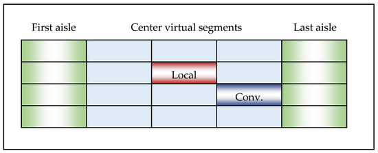
Figure 3.
Virtual segments on a planogram.
Based on the given SVS numbers, we calculate (), which defines the left () and right () horizontal coordinates of the virtual segment. The size of the special virtual segments is flexible. This means that the virtual segment may be reduced, extended or moved left or right, but the centre of each special product must be placed inside the original left and right borders of the SVS. Figure 4 demonstrates the possible sizes of the virtual segments on a planogram. On the first (lowest) shelf, the first aisle virtual segment is extended, and the space for the centre virtual segment is reduced. On the second shelf, the last aisle virtual segment is reduced, and the space for the centre virtual segments is extended. On this shelf, the convenience virtual segment is also extended. On the third shelf, the local virtual segment is reduced, the centre virtual segments are extended. On the fourth (highest) shelf, there are no changes in segments sizes.
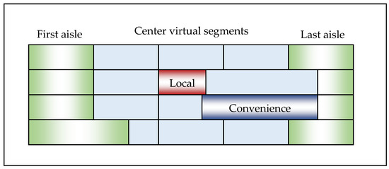
Figure 4.
Extended and reduced virtual segments on a planogram (1).
The left and right coordinates of the SVS are calculated as follows:
—for local virtual segment;
—for convenience virtual segment;
—for shelf center;
—for first aisle;
—for last aisle.
Figure 5 presents the possibilities for the extension and reduction of the SVS. If the product must be placed in any SVS, this means that the centre coordinate of a product is inside the particular virtual segment on the shelf, characterized by coordinates . The shelf is divided into virtual segments, the width of each one equals . The number of products are divided into three subsets.
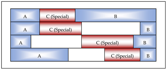
Figure 5.
Extended and reduced virtual segments on a planogram (2).
Figure 6 presents the possibilities for extending and reducing the first and the last aisle virtual segments. If the product must be placed in the first aisle, the centre coordinate of a product is inside the first virtual segment on the shelf, characterized by coordinates . Otherwise, if the product must be placed in the last aisle, the centre coordinate of the product is inside the last virtual segment on the shelf, characterized by coordinates . Figure 6 also demonstrates a shelf without special products assigned to the last aisle SVS. A similar situation may exist with other SVS types (local, convenience, shelf centre, first aisle) if there are not enough special products or are assigned to other shelves.
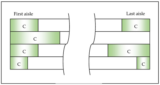
Figure 6.
Extended and reduced aisle virtual segments on a planogram.
In this research, the facings in vertical dimensions on the shelf are not taken into account. It is assumed that shelf height limit and product supply limit concern only one top row of facings with capping or nesting on it, i.e., only one row of facings is considered. The depth of the products and the shelf depth are omitted.
To solve the allocation problem, one has to determine the number of facings , a number of cappings , and a number of nestings of a product allocated to the shelf concerning a large number of constraints, which can be grouped into four categories: shelf constraints, shelf type constraints, product constraints, and virtual segments constraints. Moreover each product must be assigned to the appropriate type of the subset (i.e., subsets before (A), after (B) or inside (C) the SVS) on the shelf , . The goal is to determine the number of product allocated on the shelf to maximize profit.
4. Problem Formulation
The problem can be formulated in a condensed form as the following integer linear programming model:
, , .
—the number of facings of the product () on the shelf ().
—the number of cappings of the product () on the shelf ().
—the number of nestings of the product () on the shelf ().
,
, , , .
—the subset A, subset before the SVS on the shelf ().
—the subset C, subset inside the SVS on the shelf ().
—the subset B, subset after the SVS on the shelf ().
—the local product;
—the convenience product;
—the shelf centre product;
—the first aisle product;
—the last aisle product.
4.1. Shelf Constraints
Constraint (2) provides that the height of each product on a shelf satisfies the shelf height limit.
It is assumed that the capped products are oriented so that their width will represent the additional height to the facings of the product. The total height equals the sum of the product height, cappings height (Figure 1) and nestings height (Figure 2). Construction like omits the division by 0 situations if the product is not placed on the shelf.
Constraint (3) restricts the shelf weight limit. Constraint (4) assures the shelf length limit. Obviously, the minimum facings’ width and weight are less than the corresponding shelf length and weight limit.
4.2. Shelf Type Constraints
The following shelf type constrains have been assumed:
Constraints (5) and (6) indicate whether the product is to be placed on a pallet. If the product must not be placed on a pallet () or shelf type is not a pallet (), then . The product may be placed on a pallet if it is assigned to the pallet () and the shelf type is a pallet ().
Constraint (7) demonstrates whether the product must be placed at eye level. If the product must be placed at eye level () and the shelf is not at eye level (), then the product cannot be placed there. Other products can be placed at eye level too, so there are no restrictions for the products that are not assigned to the eye level ().
Constraint (8) shows whether the product must be placed at a lower level. If the product must be placed at a lower level () and the shelf is not at a lower level (), then the product cannot be placed there. Other products can be placed at a lower level too, so there are no restrictions for the products that are not assigned to the lower level ().
Constraint (9) signifies if the product must be placed on the shelf where the virtual segment for convenience products exists. If the product must be placed in the virtual segment for convenience products () and the shelf does not contain convenience virtual segments (), then the product cannot be placed on this shelf. If there is enough space on the shelf, regular products may also be placed here, so there are no restrictions for the products that are not assigned to the convenience zone ().
Constraint (10) indicates whether the product must be placed on the shelf where the virtual segment for local products exists. If the product must be placed in the virtual segment for local products () and the shelf does not contain a local virtual segment (), then the product cannot be placed on this shelf. If there is enough space on the shelf, regular products may also be placed in this zone, so there are no restrictions for the products that are not assigned to the local zone ().
4.3. Product Constraints
The following product constrains have been assumed:
Constraints (11) and (12) restrict the lower and upper bounds of the number of shelves on which the product should be placed. Constraint (13) ensures that the supply limit of a product is not exceeded. Constraints (14) and (15) guarantee the lower and upper bounds of product facings while (16) and (17) provide the bounds of side cappings per position. Constraint (17) ensures that the number of facings of the product is enough for the capping, i.e., the product may be capped. Constraints (18) and (19) limit the lower and upper bounds of nestings per facing position. Definition parameter (20) shows that only cappings or nestings for a product may present, but not both of them.
4.4. Virtual Segment Constraints
The following virtual segment constrains have been assumed:
Constraint (21) ensures that a non-special product belongs to the subset A or B if it is placed on the shelf. Constraint (22) ensures that a special product belongs to the subset C if it is placed on the shelf. Constraint (23) ensures that a non-special product on a local shelf belongs to the subset A or B if it is placed on the shelf. Constraint (24) ensures that a special local product on a local shelf belongs to the subset C if it is placed on the shelf. Constraint (25) ensures that a non-special product on a convenience shelf belongs to the subset A or B if it is placed on the shelf. Constraint (26) makes sure that a special convenience product on a convenience shelf belongs to the subset C if it is placed on the shelf.
Constraint (27) provides the size of the virtual segments of the shelf centre position.
The first part of the constraint (27) shows what is checked if there is too much free space on the shelf, the second part indicates regular allocation conditions when the shelf is almost full. If there is too much free space on the shelf and the number of products assigned to it is too small, there is unused space between the subsets and . Products from the subset may be allocated inside the SVS so that the centre coordinate of each product will be in the SVS. This means that the products from the subset may exceed the SVS no more than . Therefore, the maximal width of the SVS will be bounded by coordinates . The rest part of the shelf may be assigned to the subsets and . Thus, we conclude explanation of part.
If the shelf is full or almost full of products, products allocated inside the SVS can exceed its width, and there is no free space on the shelf. In other words, only the centre of the special product must be inside the SVS, not the whole product. The notation below represents the total linear size of the products that are assigned to the subsets . Here, we enumerate all possible cases:
- —the right end of the subset must be after the left coordinate of the SVS.
- —the right end of the subset must be before the right coordinate of the SVS.
- —the remainder subset must be placed in the remaining part of the shelf, not occupied by the subset , or to the right from . Parameter ensures that in case of free space between , the centre coordinate of the special product will remain inside the coordinates of the SVS.
Hence, we conclude the explanation of part.
Constraint (28) provides the size of the first aisle virtual segments. The maximum enlargement of the first aisle SVS is possible if the centre of the product is located in . Because the product may exceed the first aisle SVS by no more than half of its width, the maximum first aisle products width is . The total width of the three subsets must not exceed the shelf length, so .
Constraint (29) provides the size of the last aisle virtual segments. The maximum enlargement of the last aisle SVS is possible if the centre of the product is located in . Because the product may exceed the last aisle SVS no more than a half of its width, the maximum last aisle products width is . The total width of the three subsets must not exceed the shelf length, so .
4.5. Relationships Constraints
The following relationship constrains have been assumed:
Constraints (30) and (31) indicate facings relationships, (32) demonstrates capping relationships, (33) guarantees nesting relationships, and (34) ensures assigning products to the appropriate subsets and SVS relationships.
4.6. Decision Variables
The following decision variables have been assumed:
The binary decision variable (35) indicates if the product is placed on the shelf . Decision variables (36)–(38) result in a number of facings, cappings, and nestings of the product on the shelf are integers bounded by the given maximal values. The binary decision variable (39) indicates if the product is assigned to the subset of type on the shelf .
5. Genetic Algorithm
This research uses a classical framework of the genetic algorithm (GA) [39]. In this study, the fitness function is represented by the total planogram profit, which is equal to the sum of the unit profits of all facings, cappings, and nestings of products that are placed on all shelves on a planogram. If the solution (obtained as a result of mutation, crossover, or improvement operations) does not satisfy the constraints for any one of the totals of product length, weight, or height, or another product, shelf type or allocation constraint, then a repair mechanism that deletes product units is executed. The GA is repeated until the termination criteria are met.
5.1. Solution Representation
The solution to assigning products to shelves is represented by a chromosome, in which each gene denotes whether a product is placed on a shelf and the number of units to be placed there. The total number of genes equals the number of products multiplied by the number of shelves. This means that there is a place reserved for each product on each shelf, but if constraints are not met, the corresponding gene remains empty and the product is placed on another shelf. The population is designed as an array of individuals. Each individual is an object representing possible product allocations on virtual segments.
Figure 7 shows the chromosome representation of the current solution. Each gene consists of three parts: (1) whether the product is allocated to the shelf (true/false parameter), (2) number of facings of the product on the shelf, (3) number of cappings or nestings of the product on the shelf. It is assumed that products may be neither capped nor nested, or capped only, or nested only, but not both capped and nested. There is no situation where capping or nesting of a product exists, when the number of facings is 0. The algorithm assigns products to shelves but does not calculate how products are physically coordinated. It can assign products to subsets before (A), after (B) or inside (C) the SVS on the shelf and calculate the total space for these subsets, but it cannot calculate the linear coordinate or sequence of each product in them. Therefore, free shelf space in the figure representation does not mean physical free space in the real world. In real-life conditions, the shelf will be filled with products, and free shelf space will be minimal, or the free space (which may be less than the width of the facing) will be evenly distributed between the products allocated on the shelf so that they look better visually.
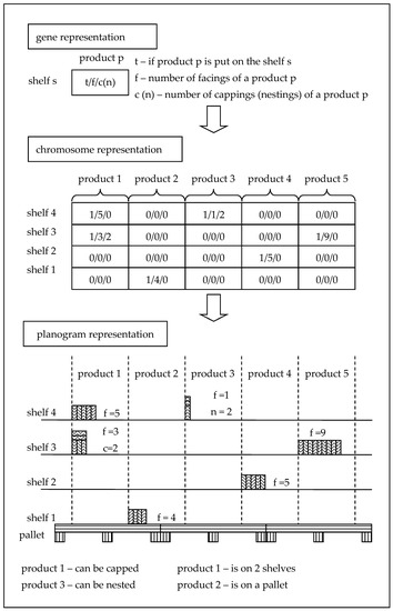
Figure 7.
Chromosome representation.
5.2. Population
At the starting point, GA creates an initial population, which contains a set of initial solutions. There are 13 types of individuals originating from 13 list algorithms. In the algorithms explained below, the first letters mean the selection priority, and the letters after the dash mean the selection method. In the possible selection methods, the abbreviations mean:
F—select the product in the defined order, then add facings, cappings, or nestings while meeting the set of constraints for the selected product.
SF—select the product in the defined order, then add facings, cappings, or nestings, and move the product to the locked sequence, so that in the next iteration, any new facing, capping or nesting will be added to another unlocked product, with regard to its place in the ordered sequence. Unlock all products and repeat the iterations while the set of constraints are met, starting with the first product in the ordered sequence. SF differs from F because it adds one facing, capping, or nesting, step by step, to each product in the list, whereas F adds one facing, capping or nesting several times to the selected product, then goes to the next product.
FF—select the product in the defined order, considering the current situation on the shelf, i.e., how many facings, cappings, or nestings are already placed on the shelf (e.g., for F or for FF), add facings, cappings, or nestings to the product, while the set of constraints are maintained. FF differs from F because F only considers the properties of one item, regardless of the number of items on the shelf.
FSF—a combination of FF and SF—select the product in the defined order, considering the current situation on the shelf, i.e., how many facings, cappings, or nestings are already placed on the shelf, then add facings, cappings, or nestings, and move this product to the locked sequence so that, in the next iteration, any new facing, capping or nesting will be added to another, unlocked, the product concerning its place in the ordered sequence. Unlock all products and repeat the iterations while the set of constraints are met, starting with the first product in the ordered sequence.
These rules are implemented in the algorithms below:
- Highest unit profit first (HUP-F)—select the product in order of non-increasing unit profit, add facings, cappings, or nestings while the set of constraints are met, and save the result value for this product in a chromosome object.
- Lowest width first (LWD-F)—select the product in order of non-decreasing width, add facings, cappings, or nestings while the set of constraints are met, and save the result value for this product in a chromosome object.
- Highest unit profit considering facings, cappings, or nestings on the shelf first (HUP-FF)—select the product in order of non-increasing on this shelf, add facings, cappings, or nestings while the set of constraints are met, and save the result value for this product in a chromosome object.
- Lowest width considering facings, cappings, or nestings on the shelf first (LWD-FF)—select the product in order of non-decreasing on this shelf, add facings, cappings, or nestings while the set of constraints are met, and save the result value for this product in a chromosome object.
- Highest unit profit to width ratio first (HUPWDR-F)—select the product in order of non-increasing unit profit to width ratio , add facings, cappings, or nestings while the set of constraints are met, and save the result value for this product in a chromosome object.
- Highest unit profit to width ratio considering facings, cappings, or nestings on the shelf first (HUPWDCNR-F)—select the product in order of non-increasing unit profit to width ratio considering facings, cappings, or nestings on the shelf , add facings, cappings, or nestings while the set of constraints are met, and save the result value for this product in a chromosome object.
- Highest unit profit considering locked sequence first (HUP-SF)—select the product in order of non-increasing unit profit, add facings, cappings, or nestings, and move this product to the locked sequence so that in the next iteration, a new facing, capping, or nesting will be added to another, unlocked, the product concerning its place in the ordered sequence. Repeat until the set of constraints are met. Unlock all products if all products are locked, and start from the first one in the ordered sequence. Save the result value for this product in a chromosome object.
- Lowest width considering locked sequence first (LWD-SF)—select the product in order of non-decreasing width, add facings, cappings, or nestings, and move this product to the locked sequence so that in the next iteration, any new facing, capping, or nesting will be added to another, unlocked, product concerning its place in the ordered sequence. Repeat until the set of constraints are met. Unlock all products, if all products are locked, and start from the first one in the ordered sequence. Save the result value for this product in a chromosome object.
- Highest unit profit considering facings, cappings, or nestings on the shelf and locked sequence first (HUP-FSF)—select the product in order of non-increasing , add facings, cappings or nestings, and move this product to the locked sequence so that in the next iteration, any new facing, capping, or nesting will be added to another, unlocked, a product with regard to its place in the ordered sequence. Repeat until the set of constraints are met. Unlock all products, if all products are locked, and start from the first one in the ordered sequence. Save the result value for this product in a chromosome object.
- Lowest width considering facings, cappings, or nestings on the shelf and locked sequence first (LWD-FSF)—select the product in order of non-decreasing , add facings, cappings or nestings, and move this product to the locked sequence so that in the next iteration, any new facing, capping, or nesting will be added to another, unlocked, product about its place in the ordered sequence. Repeat until the set of constraints are met. Unlock all products, if all products are locked, and start from the first one in the ordered sequence. Save the result value for this product in a chromosome object.
- Highest unit profit to width ratio considering locked sequence first (HUPWDR-SF)—select the product in order of non-increasing , add facings, cappings, or nestings, and move this product to the locked sequence so that in the next iteration, any new facing, capping or nesting will be added to another, unlocked, a product with regard to its place in the ordered sequence. Repeat until the set of constraints are met. Unlock all products, if all products are locked, and start from the first one in the ordered sequence. Save the result value for this product in a chromosome object.
- Highest unit profit to width ratio considering facings, cappings, or nestings on the shelf and locked sequence first (HUPWDCNR-SF)—select the product in order of non-increasing , add facings, cappings, or nestings, and move this product to the locked sequence so that in the next iteration, any new facing, capping, or nesting will be added to another, unlocked, a product with regard to its place in the ordered sequence. Repeat until the set of constraints are met. Unlock all products, if all products are locked, and start from the first one in the ordered sequence. Save the result value for this product in a chromosome object.
- Random—selects the product randomly, adds facings, cappings, or nestings while the set of constraints are met and saves the result value for this product in a chromosome object.
The whole algorithm’s name consists of the name above and a number that stands for the position of the product in the ordered sequence. For example, HUP-F1 means to select the product in order of non-increasing unit profit and use the first one (i.e., the best one); while HUP-F2 means to select the product in order of non-increasing unit profit and use the second one (i.e., the second-best one). For Random, there is no position number.
In the designed SSAP algorithm, a set of possible solutions is constructed. The number of solutions equals the population size, which is set in the GA parameters.
These are the steps in the construction of the solution:
- Set minimal possible values according to the lower bound constraints (this only concerns the initial solution step, not other steps).
- Extract facings, cappings, and nestings from the solution while the upper bound and other constraints are not met (correcting the solution after the crossover, improvement or mutation steps).
- Set minimal possible values for the products that have been completely excluded from all shelves (on previous steps), find appropriate shelves for them (correcting the solution after the crossover, improvement, or mutation steps).
- If needed, extract redundant facings, cappings, and nestings (correcting the solution after the crossover, improvement, or mutation steps).
- Add facings, cappings, and nestings to the solution according to the initial list algorithm while all constraints are met (all steps).
- Calculate fitness function (all steps).
- Assign products to the appropriate subsets A, B, C on the shelves (all steps).
5.3. Pallet Solution Recursion
The products that must be placed on a pallet shelf cannot be allocated to the other shelves, so there is only one shelf available for the pallet products. Allocating products to this pallet shelf corresponds to selecting items in a knapsack problem. In knapsack problems, a subset of items is chosen, each of which is characterized by a specific weight and value so that the resultant total value is maximized without exceeding the capacity of the knapsack. In other words, the total weight of selected items must not exceed the predefined capacity of the knapsack. Even the simplest discrete model is binary NP-hard. Most of the Knapsack problems considered are key pseudo-polynomially solvable [40].
In our case, each product has its facing width (weight) and the unit profit (value) achieved after selling this product. The shelf length represents the related weight limit of the knapsack. Because of this, we implemented a knapsack-like algorithm for the pallet. Dynamic programming is one of the exact methods for solving the knapsack problem.
We implemented a recursive algorithm that solved the classical knapsack problem with the shelf length constraint and then stored the values in an auxiliary table. The auxiliary table has a number of rows equal to the number of products and a number of columns equal to shelf length (i.e., different size values from 0 to maximum shelf length with step 1). The table models the situation when the knapsack is empty, with 0 size and the bottom-right cell models the situation when the knapsack size is the maximum possible, and it is full of items so that there is no free space on the shelf.
In the next step, we added the constraints of a limited number of facings (14) and (15). Next, we added grouping possibilities, i.e., if products are only represented by facings, or facings and cappings, or facings and nestings, and added the constraints (16)–(19). Adding a group of facings with cappings, and facings with nestings, models the situation when there is a “bonus” if we select more of the same products, i.e., when we add capping or nesting, the knapsack capacity is not reduced, but the profit is increased. Evidently, constraints (11) and (12) are satisfied because we have only one shelf for pallet type products. Constraint (13), which restricts the supply limit of the products, can also be recalculated into the notion of facings, facings and cappings, and facings and nestings. There are no virtual segments on a pallet, so it is not necessary to add virtual segment constraints here. This finishes our dynamic programming algorithm section.
In this study, the pallet has more constraints than the general knapsack. We added the shelf weight limit constraint to the recursive algorithm proportionally to each value of the shelf length. After including the shelf height constraint (2), the subset of items represented by facings, facings and cappings, and facings and nestings was recalculated. Obviously, the constraint (2) can be implemented more easily. All pallet products must be placed on a pallet. The facings number never equals 0, so there is no need to write the omitting division by 0 constructions. To save time, we subtract from the item set all lower bound values for placing them on a shelf, we reduce the shelf size (length and weight), and process only the remaining size of the shelf as the knapsack capacity. So, at this point, the auxiliary table does not represent all length and weight parameters, groups of facings, cappings or nestings. This algorithm solves the pallet part of the main problem very fast, but the solution may be not optimal. For this reason, the list algorithms are implemented on a pallet, generating a set of different solutions (they are fast enough), and a pallet also takes part in the crossover procedure. There are separate crossover methods for pallet solutions and for regular shelves.
5.4. Recombination
In this research, the mating population is created by three recombination procedures. These are: Two Rankings, Roulette Wheel, Tournament. The Two Rankings selection method [41] ranks according to decreasing total planogram profit and decreasing total free space on shelves. The total planogram profit is the sum of profits of products allocated on all shelves. The total free space on shelves is the sum of free space on all shelves remaining after product allocation. One parent individual is taken from the profit ranking and the second one from the free space ranking based on the crossover rate. The Roulette Wheel selection [41] method is based on parent individuals randomly chosen with a probability corresponding to its total profit. The common Tournament is feasible for an arbitrary group size which is called tournament size [42,43]. The Tournament method is represented as a binary tournament between two individuals based on the crossover rate.
5.5. Crossover Significant Details
In this study, both two-point and single-point crossover methods are implemented. The crossover method is selected randomly with probability 1:3 for two-point crossover and 2:3 for single-point crossover.
The point for crossover is possible if the parts of a chromosome differ at least one gene before or after it, so after the crossover, a new solution definitely appears. Otherwise, if the first or the last parts of the chromosome are the same, we will get the same solution as the initial one, so these discontinuity points are excluded from the possible crossover points. In this step, we select only appropriate discontinuity points to not waste time on. We select only appropriate discontinuity points to not waste time checking and correcting the solution after the crossover, as we definitely know in advance that an appropriate new solution will not appear.
Based on the problem’s specific character, some products can be placed only on a pallet (the lowest shelf) and other products only on regular shelves, so the crossover procedure is done separately for pallets and for regular shelves. The discontinuity point selection procedure searches separately for possible crossover points in the pallet parent variants and regular ones. Obviously, the number of pallet variants may be less than the number of the regular ones; therefore, the pallet parent variants are evenly cloned in order to get the missing number of parent individuals before the crossover.
After the crossover procedure, some equal offspring may appear because of the low diversity of genes in the selected parents. The cleaning procedure that selects only the distinct individuals is executed (not only after the crossover but also after improvement and mutation procedures) in order not to transfer redundant individuals to the next steps.
5.6. Improvement
5.6.1. General Steps
This part provides the practical guidelines for improving a developed solution. The improvement procedure for regular shelves executes on products that are not assigned to any local or convenience virtual segments or not at eye level. It moves the least profitable products to other shelves and takes more profitable products from other shelves (compared to the shelf that is under correction), and assigns an appropriate number of product items to this shelf so that the criteria value is increased.
In the product lists, the following abbreviations are used:
- GT—product is good for this shelf.
- BT—product is bad for this shelf.
- GO—product is good for other shelf.
- BO—product is bad for other shelf.
The improvement procedure executes as follows.
- Select the shelf which needs to be improved:
- If the previous step of GA is less than the result of the fitness function, select the shelf with the least criteria value.
- If there is no improvement of the GA fitness function on the last step, select any regular shelf except the shelf that was under improvement on the previous step.
- Generate a list of bad products on this shelf.
- Generate a list of good products on this shelf.
- Apply the appropriate product movement between shelves to increase the criteria value:
- Remove bad products from the shelf:
- ○
- Move bad products to another shelf if the criteria value on that shelf is better.
- ○
- Move good products to another shelf if the criteria value on that shelf is better.
- Add good products from another shelf to the selected shelf with the least criteria value (from step 1):
- ○
- Add GT from another shelf.
- ○
- Add GO from another shelf.
- Swap products on this shelf with the products on the other shelf (thisother).
- ○
- Swap BTGT.
- ○
- Swap BTGO.
- ○
- Swap GTGO.
- ○
- Swap GTGT.
- ○
- Swap BTBO.
- ○
- Swap BTBT.
- ○
- Swap GTBO.
- ○
- Swap GTBT.
- Change the number of facings on the shelf.
- ○
- Set LB values to bad products (reduce the number of facings of the bad products to LB), set UB values to good products (increase the number of facings of good products to UB) on the shelf selected in step 1.
- ○
- Subtract 1 facing from bad products (reduce the number of facings of bad products by 1), add 1 facing to good products (increase the number of facings of good products by 1) on the shelf selected in step 1.
- Remove duplicates from the set of generated solutions.
- Evaluate the set of solutions.
5.6.2. Shelf Profit Increasing
This part uses general steps in order to increase shelf profit. In this part of the paper, the following notation will be used:
- —the ratio of the shelf ().
- —the ratio of the product ().
In the increasing shelf profit step, the improvement procedure is modified as follows:
- Select the shelf with the lowest shelf ratio.
Shelf ratio equals:
Product ratio which is placed on this shelf equals:
If there is no improvement of the GA fitness function on the last step, select any regular shelf except the shelf which was under improvement on the previous step.
- 2.
- Bad products are .
- 3.
- Good products are .
- 4.
- Apply the appropriate product movement between shelves in order to increase the shelf ratio .
- 5.
- Remove duplicates from the set of generated solutions.
- 6.
- Evaluate the set of solutions.
5.6.3. Free Shelf Space Reduction
In the free shelf space reduction step, the improvement procedure is modified as follows:
- Select the shelf with the lowest total products width (maximum free space on the shelf).
If there is no improvement of the GA fitness function in the last step, select any regular shelf except the shelf which was under improvement in the previous step. Compare the product width with the average products width on the shelf.
- 2.
- Bad products are .
- 3.
- Good products are .
- 4.
- Apply the appropriate product movement between shelves in order to reduce free shelf space.
- 5.
- Remove duplicates from the set of generated solutions.
- 6.
- Evaluate the set of solutions.
5.7. Evaluation and Correction
Evaluation and correction is performed as follows. First, the algorithm deletes the redundant product item from the shelves where the constraints are not met. Next, it adds missing product items to the shelves where values are less than the lower bound. Later, it adds as many items as possible, where the criteria are met, based on the selected algorithm.
Suppose the GA fitness function is not improved compared to the previous step. In that case, a set of different individuals is generated by the pallet-like recursive algorithm, which is added to the solution set. For this reason, distinct product to shelf allocation variants is used. Next, a part of the obligatory set of product items is extracted, reducing the remaining space on the shelf. The remaining space on the shelf and the remaining part of the set of products are processed recursively like a pallet. Next, the solution is corrected. A set of solutions generated by all the list algorithms is also added to the individuals set. In ordinary cases, where GA fitness function is improved on each step, solutions are corrected only via HUPWDR-F1 algorithm. At each step, it is possible for excess solutions to be generated. Therefore, duplicates and the least profitable solutions are excluded from the set, in order not to waste time on correcting them, the necessary number of possible solutions are generated on the improvement step steering by the GA parameters.
Inside the improvement procedure, evaluation is based on the shelf ratio to the shelf length:
However, when the improved procedure has finished generating the solution set, the evaluation is based on the shelf ratio to the actually occupied space on the shelf.
After the solution correction, the evaluation is performed using the total profit on all shelves.
5.8. Mutation
The above recombination process generates new sets of chromosomes by taking the high-quality genes from the parent population. The mutation process creates a new gene in the existing chromosome. In the current GA, there are nine mutation techniques, all of which are applied to the individual selected according to the mutation rate.
In the explanation below, the terms “all shelves” and “all products” mean that all shelves and all products may be mutated, but the number of changes is limited by the mutation repetition number in the settings, i.e., not all shelves and all products will be mutated because this could destroy the solution. Therefore, before the mutation, the shelf list and product list are randomized so that they start at different places in the chromosome, thus only a few genes are mutated, not all of them. Changes in a product’s facings number trigger a recalculation of its cappings and nestings. After addition, the total number of facings cannot exceed , and the total number of facings after deletion cannot be less than . Products on which correct modifications cannot be executed so that , are omitted.
The nine mutation algorithms are:
- Mutation 1 swaps the minimum and maximum facings between products on all shelves. This action is repeated a predefined number of times (choosing maxmin, second-maxsecond-min, third-maxthird-min, and so on). Individuals are mutated in accordance with the mutation rate. Next, the minimum and maximum numbers of product facings on the shelf are chosen. The products with the least facings on this shelf increase their facings to the maximum value, and the products with the most facings reduce their facings to the number of the previously found minimum. Swapping facings also includes swapping that product’s cappings and nestings, i.e., cappings and nestings are recalculated according to the new facings number.
- Mutation 2 reverses the number of facings of all products (the predefined number of products) on all shelves around. The first product takes the number of facings, cappings and nestings of the last product, and the last product takes the number of facings, cappings and nestings of the first one.
- Mutation 3 left rotates the number of facings, cappings, and nestings of all products (the predefined number of products) on all shelves around the randomly selected product number.
- Mutation 4 swaps shelves for those products that can be placed on other shelves. This is repeated a predefined number of times, equal to the number of the swapped products.
- Mutation 5 deletes one facing without capping and adds one facing to the products where capping may be placed on all shelves for all products (the predefined number of products).
- Mutation 6 deletes one facing where the numbers of facings equal the upper bound and adds one facing where the numbers of facings equal the lower bound on all shelves for all products (the predefined number of products).
- Mutation 7 is a modification of Mutation 6 that selects not one but a randomly selected number of facings in the diapason for addition and for deletion.
- Mutation 8 selects the products with the maximum number of facings on the shelf, deletes one facing from all of them (obviously where ), selects the same number of products in their non-decreasing number of facings order on the same shelf, and adds one facing to them where .
- Mutation 9 is a reversed version of Mutation 8. It selects the products with the minimum number of facings on the shelf, adds one facing to all of them where selects the same number of products in their non-increasing number of facings order on the same shelf, and deletes one facing from all of them where .
5.9. Chromosome Correction
The solution attained after mutation and recombination is checked to see if it satisfies the defined constraints and corrected if necessary and when possible. If the current solution exceeds the predefined limits, the product cappings, nestings, and facings are extracted from the shelf until constraints are met, or it is impossible to delete product items anymore.
The individual object has a special field where the initial algorithm that generates the solution is stored. Mostly, the 13 algorithms introduced earlier are used as the initial ones. All iterations in subsequent steps are performed with the HUPWDR-F1 algorithm, which is the most profitable one. However, if the total GA iteration cannot improve the previous step’s solution, then algorithms on all individuals are reassigned, using 13 algorithms that are evenly distributed. After successful solution improvement, HUPWDR-F1 has applied again to all individuals.
The correcting procedure consists of two phases. First, minimum values are set into the solution obtained from the recombination, improvement and mutation procedures, where these values are less than the defined lower bounds. Second, redundant product items are extracting: this deletes product items if they exceed the upper bound constraints.
The following parameters are set to minimum values if they are below the lower bound values:
- Facings LB—if the product’s number of facings is less than the minimum feasible facings for the product, it is set to the lower bound.
- Cappings LB—if the product’s number of cappings is less than the minimum feasible cappings for the product, it is set to the lower bound.
- Nestings LB—if the product’s number of nestings is less than the minimum feasible nestings for the product, it is set to the lower bound.
- Shelves LB—if the shelf number where the product is placed is less than the minimum shelf number for the product, the product is placed on other shelves until the lower bound value is not met.
The extraction order is based on the algorithm currently assigned to the individual (HUPWDR-F1 or any of the 13 possible ones). If it is not possible to correct a solution or any constraint from the set does not fit, and the next product item extraction is impossible, this chromosome is deleted from the population.
The following constraints are checked:
- Shelf constraints:
- Shelf length—whether the total width of products on each shelf exceeds the shelf length limit;
- Shelf height—whether the max height of products on each shelf exceeds the shelf height limit;
- Shelf weight—whether the total weight of products on each shelf exceeds the shelf weight limit;
- Shelf type constraints:
- Pallet—whether the shelf is a pallet and products placed on it must be placed on a pallet;
- Eye level—whether the shelf is at eye level and products placed on it must be placed at eye level;
- Low level—whether the shelf is at a low level and products placed on it must be placed at low level;
- Product constraints:
- Facings UB—whether the product’s facings exceed the maximum facings for the product.
- Cappings UB—whether the product’s cappings exceed the maximum cappings for the product.
- Nestings UB—whether the product’s nestings exceed the maximum nestings for the product.
- Shelves UB—whether the shelf number where the product is placed exceeds the maximum shelf number for the product.
- Supply limit—whether the sum of the product’s facings, cappings or nestings exceeds the supply limit.
- Position allocation constraints:
- First aisle products—whether the shelf product kit allows for the first aisle products to be placed near the first aisle.
- Last aisle products—whether the shelf product kit allows for the last aisle products to be placed near the last aisle.
- Shelf center products—whether the shelf product kit allows the shelf center products to be placed in the shelf center.
- Convenience products—whether the shelf product kit allows for convenience products to be placed in the virtual segment for convenience products.
- Local products—whether the shelf product kit allows for local products to be placed in the virtual segment for local products.
- Product item is locked and cannot be extracted if, after extraction, constraints are not met.
- Facings LB—facings of the product are locked if, after extraction, the number of facings is less than the minimum facings for the product.
- Cappings LB—cappings of the product are locked if, after extraction, the number of cappings is less than the minimum cappings for the product.
- Nestings LB—nestings of the product are locked if, after extraction, the number of nestings is less than the minimum nestings for the product.
- Shelves LB—the shelf numbers of the products are locked if, after extraction, the number of shelves where the product is placed is less than the minimum shelf number for the product.
5.10. Next-Generation Selection and Termination Conditions
The best individuals according to the GA fitness function (located at the top of the sorted by non-increasing total planogram profit order) are selected for the next generation. It is supposed that the size of the new offspring, improvement and mutation population, generated by the recombination, improvement and mutation procedures, equals the size of the initial population. Similar solutions are deleted. The resulting number can be less than the population size due to the crossover and mutation rates, or if some individuals were deleted in the previous correcting step because it was impossible to correct them and satisfy the defined constraints.
In the GA, a new population of individuals is reproduced with the help of crossover, improvement, and mutation operations until the stop criteria occur. The GA stops after exceeding the maximum number of generations or the maximum number of generations without improvement of the criterion value (total planogram profit).
6. Computational Experimental Results
The computation experiments estimate the quality of the solution of the developed genetic algorithm for the SSAP. There is no real-world data available due to commercial confidentiality. Therefore several simulated problems were generated. The unit profits of the products were created randomly by a normal distribution as described by Yang [18] and Bai and Kendall [4]. The widths, heights, and weights of the products were also generated by a normal distribution. Product parameters are shown in Table 1.

Table 1.
Product parameters.
According to Yang’s experiment [18], the problem size is a significant factor in algorithm performance. Therefore, in this research, we use five sets of problem instances of different problem sizes. It is assumed that there are five stores. In each store, a specific planogram must be allocated. There is different shelf space available in each store, but the set of products that must be allocated on the shelves is the same.
For this reason, we generate five planogram product sets. All shelves on the planogram have the same length, usually the case in a real store. Very rarely do the shelf lengths differ within the same planogram. The shelf lengths in each store are: 100 cm, 200 cm, 250 cm, 375 cm, 500 cm. The numbers of products that must be allocated on four shelves on the planogram are: 10, 15, 20, 25, 50.
We also consider the influence of shelf space availability, shelf capacity, and shelf feasibility in the algorithm. Because each product has lower and upper bounds for facings, cappings, and nestings, the available shelf space must be greater than the minimum shelf space required if all products get their minimum possible values of facings, cappings, and nestings. The GA solutions were compared to the CPLEX, restricted to the time in which GA finds the solution.
The computational experiments were implemented in Visual C# 2015—Microsoft Visual Studio Community 2015 Version 14.0.25431.01 Update 3, Microsoft. NET Framework Version 4.6.01055. An optimal or feasible solution was found in IBM ILOG CPLEX Optimization Studio Version: 12.7.1.0.
6.1. Tuning of the Genetic Algorithm
A tuning process on small instances preceded GA testing. This helps to figure out control parameter values, which guarantee the highest efficiency for the chosen metaheuristic method. For this reason, each set of products on a four-shelf planogram with the shelf length equal to 250 cm are used.
The following GA parameters were set:
- Number of tests = 20;
- Population size = 3 × 13 (13 algorithms, take the 1st, the 2nd, the 3rd product according to the algorithm);
- Number of products = 10;
- Number of shelves = 4;
- Shelf length = 250 cm;
- Termination condition:
- Maximum number of iterations = 50;
- Number iterations without improvement = 0.
- While performing GA tuning such control parameters are tested:
- Crossover rate = {0.1, 0.2 ... 1.0};
- Mutation rate = {0.01, 0.02 ... 0.1};
- Selection method = {Two Rankings, Roulette Wheel, Tournament}.
As a result of the tuning process, the configuration parameters listed in Table 2 were found. We provide clarification of several parameters in Table 2, where the following abbreviation are used: TR—Two Rankings; RW—Roulette Wheel; T—Tournament.
Table 2.
Tuning parameters.
6.2. Genetic Algorithm vs. CPLEX
Tuning was performed without the improvement parameters and with the improvement procedure because the goal was to select the most profitable parameters regardless of the improvement procedure. The improvement procedure was applied in the second stage of the developed algorithm. Moreover, the aim was also to compare the quality of GA with and without the improvement procedure.
As shown in Table 3, the Tournament selection method gives a more profitable result (without improvement). Because Tournament is a two-stage selection of the better results, it provides the least amount of different selected solutions in the end. The Two Rankings selection method selects the largest number of different solutions because they are based on the two sorted sequences. Roulette Wheel selects a medium number of distinct solutions because the most profitable solutions are selected more frequently. At this point, we predicted that Two Rankings would be the best choice to test the improvement procedure, and therefore we decided to test and compare all three selection methods. For evaluating the GA solution, 20 tests were done for each problem size instance.
Table 3.
Quality of the best solution of GA+ compared to the CPLEX solution (Time_CPLEX = Time_GA).
In this part of the paper, the following notation will be used:
- GA−—GA without the improvement procedure;
- GA+—GA with the improvement procedure;
Table 3 presents the quality of the GA+ solution compared to the CPLEX solution. The best solution with the maximum total profit has been selected from the testing sets. CPLEX was run limited by the time taken for the result of GA+ to be found.
It should be noted that GA+ with Two Rankings and GA+ with Roulette Wheel were better in 18 cases out of 22. GA+ with Two Rankings was better than CPLEX by approximately 1.83%, with its minimum and maximum values 0.05% and 7.03%, respectively. GA+ with Roulette Wheel was better than CPLEX by approximately 1.53%, with its minimum and maximum values 0.03% and 7.05%, respectively. In three cases, CPLEX found the same solution as GA+ with Two Rankings and GA+ with Roulette Wheel. GA+ with Tournament was also better in 16 cases out of 22 than CPLEX by approximately 3.49%, with its minimum and maximum values 0.03% and 27.07%respectively. In five cases, CPLEX found the same solution as GA+ with Tournament.
Figure 8 presents the computational time for the best solution of GA+. GA+ with Tournament was the fastest and found the solution on average in 2.52 min with its minimum 0.01 min and maximum 10.39 min values. GA+ with Roulette Wheel was the slowest, averaging 3.29 min with its minimum and maximum solutions of 0.02 min and 40.63 min, respectively. GA+ with Two Rankings found the solution in 2.81 min on average, with its minimum 0.02 min and maximum 27.15 min values.
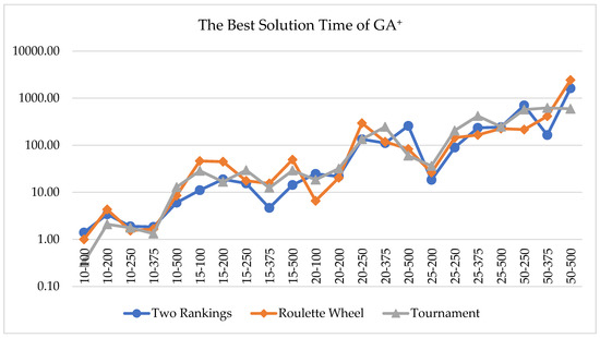
Figure 8.
The computational time for the best solution of GA+ in [s].
The question arises: why are the results for GA+ with Tournament for the set of 10 products and shelf sizes 200 cm and 375 cm so much higher (14.31%, 27.07%) than the CPLEX solution compared to the other methods? As written above, the Tournament selection method gives the least number of distinct solutions. The bulk of the time is spent in checking and correcting the solution, i.e., if the criteria are not met, the procedure deletes redundant product items, and then the procedure adds product items where the requirements are met. The problem for allocating 10 products is easy enough compared to larger product sets; the Tournament selection gives fewer product permutations. Thus, fewer solutions need to be checked and corrected. That is why GA+ faster finds the result (1 s for 375 cm for GA+ with Tournament compared to 2 s both for GA+ with Two Rankings and GA+ with Roulette Wheel). Thus, in 2 s, CPLEX found a significantly better solution than in 1 s. A similar situation is with 200 cm shelves. Here GA+ with Tournament found the solution in 2 s, but GA+ with Tournament compared to 2 s for GA+ with Two Rankings and GA+ with Roulette Wheel, found the solution in 3 s and 4 s, correspondingly. N.B.: CPLEX accepts seconds as integers, so the GA solution time was rounded. For the case with 15 products and 100 cm shelves, the CPLEX solution was better by 1.24% for all GAs+.
Table 4 presents the quality of the GA+ solution compared to the CPLEX solution. As previously, the best solution with the maximum total profit was selected from the testing sets. CPLEX was run, limited by the maximum time in which the result of the GA+ was found.
Table 4.
Quality of the best solution of GA+ compared to the CPLEX solution (Time_CPLEX = max_Time_GA).
It should be noted that GA+ with Two Rankings and GA+ with Tournament were better in 14 cases out of 22, GA+ with Roulette Wheel was better in 15 cases. In 7 cases, CPLEX found the same solution as GA+ with Two Rankings, in 6 cases, CPLEX found the same solution as GA+ with Roulette Wheel and GA+ with Tournament. For the case with 15 products and 100 cm shelves, the CPLEX solution was better by 1.24% for all GA+ tests; when we extend the time for the CPLEX, it also found a 0.22% better solution for 15 products set and 500 cm shelves than GA+ with Tournament. Both GA+ with Two Rankings and GA+ with Tournament found the solution better than CPLEX by an average of 1.33%, with its minimum and maximum values 0.03% and 7.03%. GA+ with Roulette Wheel found the solution slightly higher, on average 1.74% better than CPLEX with minimum and maximum values 0.05% and 7.05%.
Figure 9 demonstrates the average time for GA+. All GAs+ found the solution on average approximately 2–3 min. The fastest solution was found in 0.01–0.02 min and the slowest one in 27.15 min by GA+ with Two Rankings, 40.63 min by GA+ with Roulette Wheel and 42.74 by GA+ with Tournament.
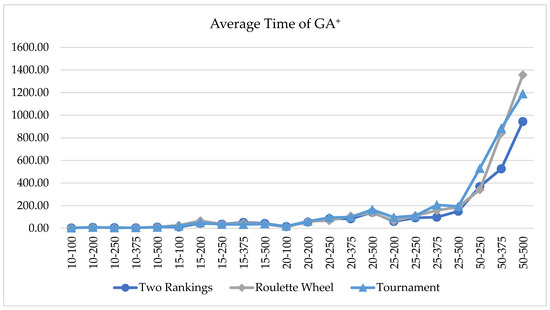
Figure 9.
Average time for GA+ in [s].
Table 5 shows the quality of the best and average solutions of GA− compared to the best and average solutions of GA+. In the case of the best solutions for the set of 10 products, GA− and GA+ found the same solution almost in all cases, except GA+ with Tournament which was better on 500 cm shelves. For all other cases, GA+ with Roulette Wheel and GA+ with Tournament were better than GA− on average 0.30% (0.03–1.58%). GA+ with Two Rankings slightly differs, finding the better solution on average by 0.28% (0.04–1.58%). In the case of average solutions in all cases, GA+ was better than GA−. GA+ with Two Rankings and GA+ with Tournament were better than the corresponding GA− on average 1.89%, but GA+ with Roulette Wheel gives the slightly higher average result 5.16%. The minimum value for GA+ with Two Rankings and GA+ with Roulette Wheel is 0.19%, and 0.28% for GA+ with Tournament. GA+ with Roulette Wheel found the highest value compared to GA− of 65.80%. Other GA+ with Two Rankings and GA+ with Tournament give 28.10% and 24.98% their maximum values.
Table 5.
Quality of the best/average solution of GA− compared to the best/average solution of GA+.
Figure 10 shows the computational time for the best solution of GA−. GA− with Tournament was the fastest, and the solution on average in 0.56 min. The minimum time for all GAs− was 0.03–0.04 min. The maximum time was approximately 2.5 min for both GA− with Roulette Wheel and GA− with Tournament, and 5.71 min for GA− with Two Rankings. All GAs− on average found the solution in less than 1 min.
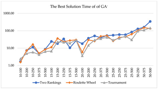
Figure 10.
The computational time for the best solution of GA− in [s].
Figure 11 demonstrates the average time for GA−. All GAs+ found the solution, on average, in less than 1 min. The fastest solution was found in less than 1 s and the slowest in 6.92 min by GA+ with Two Rankings, 5.17 min by GA+ with Roulette Wheel, and 4.33 min by GA+ with Tournament. It is significantly faster than GA+.
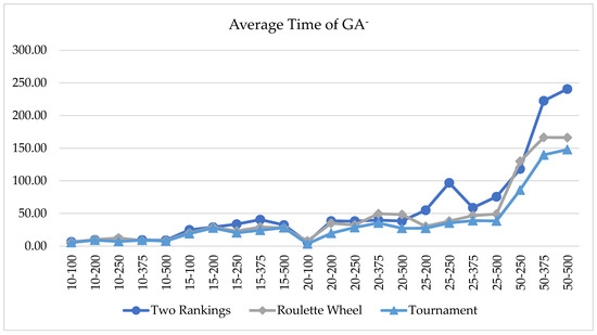
Figure 11.
Average time for GA− in [s].
Table 6 presents the standard deviation of GA− solutions compared to the standard deviation of GA+ solutions. It can be observed that GA+ finds a more stable solution set. It can improve any solution, and it is better than GA− by approximately 60–65%. The minimum and maximum values where GA+ is less varied are 23–32% and 95–97%. This means that in the best cases, GA+ is almost twice as good as GA−, and generally gives almost equal solutions. Conversely, GA− gets good solutions that significantly depend on the initial solution or on selected random values.
Table 6.
Standard deviation of GA- solutions compared to standard deviation of GA+ solutions.
7. Discussion
Shelf space is one of the most essential and difficult resources to manage in retailing. In this paper, the practical model of shelf space allocation restricted by four constraint subsets, and based on the retailer’s visual merchandising rules, is formulated with the aim of maximizing profit through a planogram. Efficient shelf space allocation increases the visibility of the products, customer satisfaction, and sales generation, which is the key point for the retailer.
Merchandising is the key driver of the visual representation of planogram in a retail store. In the retail industry, merchandising is the activity of promoting products in order to increase sales. Merchandising includes the way of displaying products in stores as well as free samples, distributing marketing materials, on-the-spot demonstration, and special offers or pricing. The aim of the merchandiser is to determine which types of fixtures, on which shelf types, and in which positions the product will be displayed. This is a very important task because incorrect product allocation negatively affects sales [35].
This research investigates an important merchandising rule of dividing shelves into segments and using horizontal and vertical ties between products and their location on the shelves, which varies between segments. Moreover, the segments are of flexible sizes.
Bianchi-Aguiar et al. [7,8] developed an automatic planogram replication tool with regard to product families. Russell and Urban [44] model the problem by specifying the position of products on the shelves and block the product families into rectangular shapes. Our approach is related to this stream and defines different types of shelf location (we name them virtual segments because the shelf is not divided physically into the segments, there are no borders between the segments, but space planners need an idea of creating such segments visually and this approach is very convenient). We also provide a method of defining such virtual segments with the centre coordinate specified and with flexible borders that could be reduced or extended.
As a solution to the introduced SSAP, a genetic algorithm has been proposed, the efficiency of which has been evaluated using the CPLEX solver. The proposed and developed enhancement solution steps provide a stable solution, and they may be used in solving category management shelf space allocation problems or another knapsack-like problems.
The presented model is similar to the knapsack problem but involves a large number of simultaneous constraints. Computation results prove that the proposed algorithm allows for obtaining very efficient results in a very short running time.
8. Conclusions
In this paper, an example of using combinatorial optimization in solving a practical problem is presented. We studied the problem of SSAP to maximize the total planogram profit. It used a practical mathematical model to generate automatic planograms that may be of different lengths in each store but allocate the same product set. We found no previous articles examining so many constraints in SSAP simultaneously; only facings had been investigated, despite real-world retailers having ever more restrictions to satisfy. This study augmented the basic SSAP model with retail merchandising tactics, resulting in a set of constraints grouped into four categories: shelf (capacity); shelf type (vertical level effect); product (regional, complementary, etc.); and virtual segment (location, grouping) constraints. It further enriched the previous models with complex product representation of facings, cappings per facings group, and nestings per facings position.
This problem is an extension of a knapsack problem classified as NP-hard, so heuristic and metaheuristic approaches were used. A GA was implemented; the most valuable part of it is the improvement procedure that provides the practical guidelines for solution enhancement. The quality of the solution was compared to the CPLEX solver.
Based on the experimental results, the GA proposed in this paper rapidly gives high-quality results for different problem instances: on average, 2.52 min for GA+ with Tournament, 2.81 min for GA+ with Two Rankings, 3.29 min for GA+ with Roulette Wheel. Interestingly, GA+ with Two Rankings and GA+ with Roulette Wheel were better than the CPLEX in 18 cases out of 22, and GA+ with Tournament was better in 16 cases out of 22 the solver within the same predefined solution time limitation. Notably, GA+ finds a more stable solution set than GA−, which is better by approximately 60–65% due to the improvement procedure. Moreover, GA+ gives 23–32% and 95–97% less result deviation, which is not highly dependent on the initial solution or random values selected.
The proposed recursive algorithm for allocating products on a shelf may be used in solving other knapsack-like problems. GA is a promising approach for solving combinatorial SSAP optimization tasks. Regarding its limitations, it only finds the possibility that the products can be physically allocated on the shelves in the defined virtual segments. Still, it does not find the products’ exact coordinates on the shelves. Another limitation is that the depth (of the shelf and product) parameter was omitted. The solution could be further expanded, also with the possibility of sorting products on the shelf according to their price, brand, category, and so on. Therefore, the directions of our further investigation include enhancing the model with the effects of uncertain demand as well as space- and cross-space elasticity effects, and including depth of products and shelves.
Author Contributions
Conceptualization, K.C., K.S.-W., and M.H.; Data curation, K.C.; formal analysis, K.C., P.S., and A.R.; funding acquisition, M.H.; investigation, K.C.; methodology, K.C.; project administration, M.H.; resources, K.C. and M.H.; software, K.C.; supervision, K.S.-W. and M.H.; validation, K.C. and M.H.; visualization, K.C.; writing—original draft, K.C.; writing—review and editing, K.C., K.S.-W., P.S., and A.R. All authors have read and agreed to the published version of the manuscript.
Funding
This research was funded by the Ministry of Science and Higher Education in Poland under the program “Regional Initiative of Excellence” 2019–2022 project number 015/RID/2018/19, total funding amount 10,721,040,00 PLN.
Institutional Review Board Statement
Not applicable.
Informed Consent Statement
Not applicable.
Data Availability Statement
Not applicable.
Acknowledgments
Not applicable.
Conflicts of Interest
The authors declare no conflict of interest.
References
- Lotfi, M.M.; Rabbani, M.; Ghaderi, S.F. A weighted goal programming approach for replenishment planning and space allocation in a supermarket. J. Oper. Res. Soc. 2011, 62, 1128–1137. [Google Scholar] [CrossRef]
- Lim, A.; Rodrigues, B.; Zhang, X. Metaheuristics with Local Search Techniques for Retail Shelf-Space Optimization. Manag. Sci. 2004, 50, 117–131. [Google Scholar] [CrossRef]
- Hwang, H.; Choi, B.; Lee, M.J. A model for shelf space allocation and inventory control considering location and inventory level effects on demand. Int. J. Prod. Econ. 2005, 97, 185–195. [Google Scholar] [CrossRef]
- Bai, R.; Kendall, G. An investigation of automated planograms using a simulated annealing based hyper-heuristic. Oper. Res. Comput. Sci. Interfaces Ser. 2005, 32, 87–108. [Google Scholar] [CrossRef]
- Drèze, X.; Hoch, S.J.; Purk, M.E. Shelf management and space elasticity. J. Retail. 1994, 70, 301–326. [Google Scholar] [CrossRef]
- Bianchi-Aguiar, T. The Retail Shelf Space Allocation Problem: New Optimization Methods Applied to a Supermarket Chain. Ph.D. Thesis, Department of Industrial Engineering and Management, Faculdade de Engenharia da Universidade do Porto, Porto, Portugal, 2015. [Google Scholar]
- Bianchi-Aguiar, T.; Silva, E.; Guimarães, L.; Carravilla, M.A.; Oliveira, J.F.; Amaral, J.G.; Liz, J.; Lapela, S. Using analytics to enhance a food retailer’s shelf-space management. Interfaces 2016, 46, 424–444. [Google Scholar] [CrossRef]
- Bianchi-Aguiar, T.; Silva, E.; Guimarães, L.; Carravilla, M.A.; Oliveira, J.F. Allocating products on shelves under merchandising rules: Multi-level product families with display directions. Omega 2018, 76, 47–62. [Google Scholar] [CrossRef]
- Frontoni, E.; Contigiani, M.; Ribighini, G. A heuristic approach to evaluate occurrences of products for the planogram maintenance. In Proceedings of the MESA 2014—10th IEEE/ASME International Conference on Mechatronic and Embedded Systems and Applications, Senigallia, Italy, 10–12 September 2014. [Google Scholar]
- Hübner, A. Retail Category Management. Decision Support Systems for Assortment, Shelf Space, Inventory and Price Planning; Lecture Notes in Economics and Mathematical Systems, 656; Springer: Berlin/Heidelberg, Germany, 2011. [Google Scholar]
- Chen, Y.K.; Weng, S.X.; Liu, T.P. Teaching-learning based optimization (TLBO) with variable neighborhood search to retail shelf-space allocation. Mathematics 2020, 8, 1296. [Google Scholar] [CrossRef]
- Geismar, H.N.; Dawande, M.; Murthi, B.P.S.; Sriskandarajah, C. Maximizing Revenue through Two-Dimensional Shelf-Space Allocation. Prod. Oper. Manag. 2015, 24, 1148–1163. [Google Scholar] [CrossRef]
- Hübner, A.; Schaal, K. A shelf-space optimization model when demand is stochastic and space-elastic. Omega 2017, 68, 139–154. [Google Scholar] [CrossRef]
- Hübner, A.H.; Kuhn, H. Retail category management: State-of-the-art review of quantitative research and software applications in assortment and shelf space management. Omega 2012, 40, 199–209. [Google Scholar] [CrossRef]
- Yu, V.F.; Maglasang, R.; Tsao, Y.C. A reduced variable neighborhood search-based hyperheuristic for the shelf space allocation problem. Comput. Ind. Eng. 2020, 143. [Google Scholar] [CrossRef]
- Urban, T.L. An inventory-theoretic approach to product assortment and shelf-space allocation. J. Retail. 1998, 74, 15–35. [Google Scholar] [CrossRef]
- Yang, M.H.; Chen, W.C. Study on shelf space allocation and management. Int. J. Prod. Econ. 1999, 60–61, 309–317. [Google Scholar] [CrossRef]
- Yang, M.H. Efficient algorithm to allocate shelf space. Eur. J. Oper. Res. 2001, 131, 107–118. [Google Scholar] [CrossRef]
- Lim, A.; Rodrigues, B.; Xiao, F.; Zhang, X. Adjusted network flow for the shelf-space allocation problem. In Proceedings of the International Conference on Tools with Artificial Intelligence, Washington, DC, USA, 4–6 November 2002; pp. 224–229. [Google Scholar] [CrossRef]
- Gajjar, H.K.; Adil, G.K. A piecewise linearization for retail shelf space allocation problem and a local search heuristic. Ann. Oper. Res. 2010, 179, 149–167. [Google Scholar] [CrossRef]
- Hansen, J.M.; Raut, S.; Swami, S. Retail Shelf Allocation: A Comparative Analysis of Heuristic and Meta-Heuristic Approaches. J. Retail. 2010, 86, 94–105. [Google Scholar] [CrossRef]
- Gajjar, H.K.; Adil, G.K. Heuristics for retail shelf space allocation problem with linear profit function. Int. J. Retail Distrib. Manag. 2011, 39, 144–155. [Google Scholar] [CrossRef]
- Bookbinder, J.H.; Zarour, F.H. Direct product profitability and retail shelf-space allocation models. J. Bus. Logist. 2001, 22, 183–208. [Google Scholar] [CrossRef]
- Reisi, M.; Gabriel, S.A.; Fahimnia, B. Supply chain competition on shelf space and pricing for soft drinks: A bilevel optimization approach. Int. J. Prod. Econ. 2019, 211, 237–250. [Google Scholar] [CrossRef]
- Baron, O.; Berman, O.; Perry, D. Shelf space management when demand depends on the inventory level. Prod. Oper. Manag. 2011, 20, 714–726. [Google Scholar] [CrossRef]
- Tsao, Y.C.; Lu, J.C.; An, N.; Al-Khayyal, F.; Lu, R.W.; Han, G. Retailer shelf-space management with trade allowance: A Stackelberg game between retailer and manufacturers. Int. J. Prod. Econ. 2014, 148, 133–144. [Google Scholar] [CrossRef]
- Zhao, J.; Zhou, Y.W.; Wahab, M.I.M. Joint optimization models for shelf display and inventory control considering the impact of spatial relationship on demand. Eur. J. Oper. Res. 2016, 255, 797–808. [Google Scholar] [CrossRef]
- Hübner, A.; Schaal, K. Effect of replenishment and backroom on retail shelf-space planning. Bus. Res. 2017, 10, 123–156. [Google Scholar] [CrossRef]
- Hübner, A.; Schaal, K. An integrated assortment and shelf-space optimization model with demand substitution and space-elasticity effects. Eur. J. Oper. Res. 2017, 261, 302–316. [Google Scholar] [CrossRef]
- Schaal, K.; Hübner, A. When does cross-space elasticity matter in shelf-space planning? A decision analytics approach. Omega 2018, 80, 135–152. [Google Scholar] [CrossRef]
- Irion, J.; Lu, J.C.; Al-Khayyal, F.; Tsao, Y.C. A piecewise linearization framework for retail shelf space management models. Eur. J. Oper. Res. 2012, 222, 122–136. [Google Scholar] [CrossRef]
- Borin, N.; Farris, P.W.; Freeland, J.R. A Model for Determining Retail Product Category Assortment and Shelf Space Allocation. Decis. Sci. 1994, 25, 359–384. [Google Scholar] [CrossRef]
- Ghazavi, E.; Lotfi, M.M. Formulation of customers’ shopping path in shelf space planning: A simulation-optimization approach. Expert Syst. Appl. 2016, 55, 243–254. [Google Scholar] [CrossRef]
- Reyes, P.M.; Frazier, G.V. Goal programming model for grocery shelf space allocation. Eur. J. Oper. Res. 2007, 181, 634–644. [Google Scholar] [CrossRef]
- Jajja, M.S.S. Retail shelf space allocation analysis using system dynamics approach. J. Qual. Technol. Manag. 2013, 9, 99–129. [Google Scholar]
- Fadiloğlu, M.M.; Karaşan, O.E.; Pinar, M.Ç. A model and case study for efficient shelf usage and assortment analysis. Ann. Oper. Res. 2010, 180, 105–124. [Google Scholar] [CrossRef][Green Version]
- Elbers, T. The Effects of In-Store Layout-and Shelf Designs on Consumer Behavior. 2016. Available online: http://edepot.wur.nl/369091 (accessed on 20 June 2021).
- Desrochers, D.M.; Nelson, P. Adding consumer behavior insights to category management: Improving item placement decisions. J. Retail. 2006, 82, 357–365. [Google Scholar] [CrossRef]
- Baeck, T.; Fogel, D.B.; Michalewicz, Z. Handbook of Evolutionary Computation; IOP Publishing Ltd.: Bristol, UK; Oxford University Press: Oxford, UK, 1997. [Google Scholar]
- Pisinger, D. Algorithms for Knapsack Problems. Ph.D. Thesis, University of Copenhagen, København, Denmark, 1995. [Google Scholar]
- Kumar, R. Jyotishree Blending Roulette Wheel Selection & Rank Selection in Genetic Algorithms. Int. J. Mach. Learn. Comput. 2012, 2, 365–370. [Google Scholar] [CrossRef]
- Blickle, T.; Thiele, L. A Comparison of Selection Schemes used in Genetic Algorithms. Evol. Comput. 1996, 4, 361–394. [Google Scholar] [CrossRef]
- Chakraborty, M.; Chakraborty, U.K. Branching process analysis of linear ranking and binary tournament selection in genetic algorithms. J. Comput. Inf. Technol. 1999, 7, 107–113. [Google Scholar]
- Russell, R.A.; Urban, T.L. The location and allocation of products and product families on retail shelves. Ann. Oper. Res. 2010, 179, 131–147. [Google Scholar] [CrossRef]
Publisher’s Note: MDPI stays neutral with regard to jurisdictional claims in published maps and institutional affiliations. |
© 2021 by the authors. Licensee MDPI, Basel, Switzerland. This article is an open access article distributed under the terms and conditions of the Creative Commons Attribution (CC BY) license (https://creativecommons.org/licenses/by/4.0/).