Computation of Optimized Electrode Arrays for 3-D Electrical Resistivity Tomography Surveys

Abstract

The present study explores the applicability and effectiveness of an optimization technique applied to electrical resistivity tomography data. The procedure is based on the Jacobian matrix, where the most sensitive measurements are selected from a comprehensive data set to enhance the least resolvable parameters of the reconstructed model. Two existing inversion programs in two and three dimensions are modified to incorporate this new approach. Both of them are selecting the optimum data from an initial comprehensive data set which is comprised of merged conventional arrays. With the two-dimensional (2-D) optimization approach, the most sensitive measurements are selected from a 2-D survey profile and then a clone of the resulting optimum profile reproduces a three-dimensional (3-D) optimum data set composed of equally spaced parallel lines. In a different approach, with the 3-D optimization technique, the optimum data are selected from a 3-D data set of equally spaced individual parallel lines. Both approaches are compared with Stummer’s optimization technique which is based on the resolution matrix. The Jacobian optimization approach has the advantage of selecting the optimum data set without the need for the solution of the inversion problem since the Jacobian matrix is calculated as part of the forward resistivity problem, thus being faster from previous published approached based on the calculation of the sensitivity matrix. Synthetic 3-D data based on the extension of previous published works for the 2-D optimization case and field data from two case studies in Greece are tested, thus verifying the validity of the present study, where fewer measurements from the initial data set (about 15–50%) are able to reconstruct a model similar with the one produced from the original comprehensive data set.

1. Introduction

Over the last twenty years, electrical resistivity tomography (ERT) has been transformed into a widely used geophysical method for approaching several different near-surface applications. This was boosted by the improvement of the hardware’s capabilities, the development of multichannel resistivity systems and the compilation of automated inversion and reconstruction algorithms to image and monitor the subsurface geoelectrical properties [1]. Two dimensional (2-D) ERT method is nowadays routinely applied in approaching diverse problems including the study of saline water intrusion in coastal aquifers [2], the tracing of water content dynamics in unsaturated zones [3], in geotechnical studies [4] and the monitoring of subsurface conductive pollutants [5].

However, 2-D approaches underperform in cases of complicated stratigraphy and intense inhomogeneity of the subsurface resistivity. Thus, significant research efforts have been placed on proposing and investigating the resolving capabilities of different measuring and processing strategies to map the subsurface resistivity structure within a three-dimensional (3-D) context [6,7,8,9,10]. Every surface or cross-hole ERT experiment involves the arrangement of a number of electrodes along a line for 2-D or on the nodes of a regular or irregular grid for 3-D resistivity surveying, respectively. In either case, the linearly independent apparent resistivity measurements are a function of the maximum number of electrodes that are simultaneously connected to any multiplexed/multichannel resistivity instrument. The number of measurements for an array using four-electrode configurations increases exponentially with the respective number of electrodes [11,12]. This renders the field collection of all the possible measurements practically impossible, even for an array composed of a relatively small number (~50) of electrodes. Thus, the routine practice relies on the collection of tomographic data using standard electrode arrays [13] and the integration of dense parallel or orthogonal 2-D lines to characterize the 3-D resistivity structure [14].

A step forward to exploit the full capability spectrum of the modern acquisition instruments was firstly introduced by the pioneering work of Stummer et al. [15], who presented an experimental optimization method to select electrode arrays that maximize the resolving capabilities of the inversion images. Their approach was based on the compilation of the comprehensive data set including all the standard and non-standard arrays, the associated resolution matrix and a goodness function that ranks the sensitivity of every possible measurement to changes in the subsurface parameters. Extensive comparisons among the reconstructed models resulting from the inversion of the comprehensive, standard, and optimized data sets revealed the significant potential of the proposed technique.

Wilkinson et al. [16] developed and tested some improved strategies for the automatic selection of the optimized ERT data sets using a linearized estimate of the model resolution matrix that quantifies the resolving capabilities of the observed data. One of the methods (Compare R) directly compared the model resolution matrices to enhance the spatial resolution while another one used a modified version of the goodness function (Modified GF) to ensure a high degree of orthogonality to the base data set. The effectiveness of the algorithms was validated through synthetic and real data, outlining their relative superiority in the optimization and resolving capabilities performance in relation to Stummer’s method, though being more time consuming than Stummer’s approach. Wilkinson et al. [17] presented an adaptive optimization method based on Compare R to compile optimum arrays for time-lapse monitoring surveys.

Loke et al. [18] addressed the time-consuming issues related to the automatic selection of the optimized data set using a fast computation strategy to reduce the traffic between the computer main memory and the CPU registers. They compared Compare R, Modified GF, hybrid Modified GF–Compare R and Stummer’s method, using synthetic and field tests. The results verified the superiority of Compare R to all the other methods. Their tests outlined that the hybrid Modified GF–Compare R method produced results almost identical to Compare R with the advantage of being several times faster.

In another work by Loke et al. [19], it is emphasized that using a smaller step to add optimized measurements to the base data set benefits the final model resolution. Furthermore, the particular study referred to the advantages of replacing matrix–vector with matrix–matrix multiplications, the storing of temporary variables in the double-precision single instruction multiple data (SIMD) registers within the CPU and the use of a computer graphics processor unit (GPU) to decrease the calculation time for selecting the optimum configurations.

In a more recent study, Loke et al. [20] presented optimized arrays for 2-D resistivity surveys with buried probes, using implanted electrodes in the subsurface and on the ground surface. This geometry array was able to increase the depth resolution of resistivity surveys at sites where the profile length is limited. Apart from the fact that the resolution is better when optimal arrays are used, the specific study also manifested the increased resolution distances slightly beyond the lateral ends of the arrays and for depths below the buried array.

Coles and Morgan [21] followed a slightly different path for the sequential experimental design of optimum resistivity data sets by developing a determinant-based objective function that minimizes the posterior model uncertainty. The aspect of computational efficiency was addressed through formulae for updating determinants and matrix inverses without the need for direct calculation. The applicability of the method was demonstrated on single and adaptive borehole ERT surveys. Additionally, Wagner et al. [22] applied a new approach based on the resolution matrix to calculate the optimal electrode positions, wherein the results of the study confirmed that a sparse but well-conceived set of electrodes can provide a large part of the information content offered by comparably dense electrode distributions.

All the above optimization algorithms rely on the appraisals of the model resolution matrix that is directly related to the calculation of the generalized inverse, which can be extremely time-consuming in large 2-D [23] and 3-D problems [14]. Furman et al. [24] recommended a method to extract the optimal set of ERT arrays using genetic algorithms to identify the array with the optimal cumulative spatial sensitivity. Athanasiou et al. [25] proposed an alternative method to pick the optimal measurements solely on the examination of the sensitivity matrix entries. The extensive testing of the specific algorithm proposed by Athanasiou et al. [25] with surface, cross-hole and surface-to-hole electrode layouts demonstrated comparable results with previously published approaches.

The extension of the optimization procedure to generate a set of optimum measurements for 3-D survey grids poses new challenges to balance the time constraints and the need to increase the resolution analysis of the 3-D subsurface inversion images. Loke et al. [26] presented the first effort of computing optimized arrays for 3-D surface electrical surveys. In the specific work, they constructed the comprehensive data set with a mixture of in-line and offset alpha and beta configurations as well as respective equatorial arrays. The unstable measurements were filtered out by setting a maximum limit for the geometric factor and the sensitivity of the array geometric factor in the position of the electrodes. A similar approach was also followed in optimizing resistivity measurements collected from the layout of electrodes placed on nodes of non-regular grids [27]. Recently Uhlemann et al. [28] presented a novel algorithm combining the optimization of measurement configuration and electrode placement both for the 2-D and 3-D case.

The present study is focused on generating the optimum 3-D tomographic resistivity data sets based on the sensitivity matrix and employing two different formulations. At first, a 2-D optimization algorithm was the basis to extract optimum arrays along a single section and the optimized 3-D data set resulting from cloning these parallel 2-D optimized sections. The second approach involved the extension of an experimental algorithm in a 3-D context and the extraction of the optimized arrays from 3-D tomographic data sets composed of a dense network of parallel 2-D lines. The resolving capabilities of the optimized configurations produced by these two different strategies were compared using synthetic data generated from the extension of a known published 2-D resistivity model in the 3-D space. In either case, the comprehensive data set was composed of a mixture of commonly known electrode arrays. Both optimization techniques are compared with Stummer’s approach. The efficiency of the 3-D optimized protocols in imaging the subsurface resistivity structure was also verified with two real field data examples from Greece.

2. Methodology

The experimental selection of the optimum measurements from an initial array based on the Jacobian matrix (see Appendix A) method was firstly introduced by Athanasiou et al. [25] for the case of the 2-D resistivity tomographic problem. The same technique expanded and incorporated within a 3-D resistivity modelling and inversion algorithm [14] to select the optimum tomographic data in the 3-D space. In both algorithms, the adjoint equation technique [29] is used to calculate the sensitivity matrix in a homogeneous 2-D or 3-D resistivity model, which associates variations in the resistivity of the parameters ρ_j with variations in the apparent resistivity data d_i. This was carried out to ensure the generality of the optimized protocols regardless of the target’s or the background’s property values.

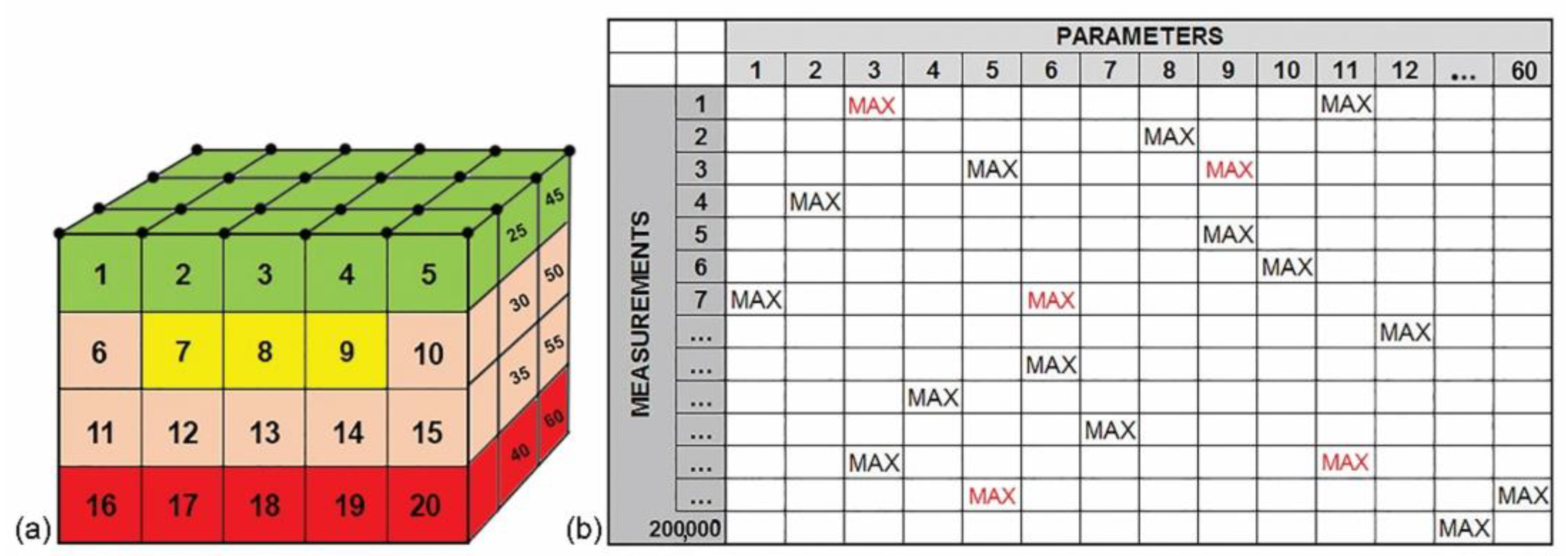
Figure 1a illustrates a simplified model with 24 surface electrodes (indicated with black dots), on a 3-D rectangular grid with the associated parameterization of the subsurface composed of 60 blocks to describe the earth’s resistivity. It is known that the parameters closer to the surface electrodes are more sensitive to any change since they have higher absolute Jacobian values (Figure 1a, green-colored blocks). Gradually, the parameters that are further away from the surface (Figure 1a, yellow-colored blocks) and to the edges (Figure 1a, red-colored blocks) are less sensitive (lower absolute Jacobian values) to any subsurface resistivity change. As an example, let us assume an experiment with 200,000 measurements collected from a network of 24 surface electrodes and a subsurface model discretized using these 60 parameters. The calculated Jacobian matrix will have 200,000 rows representing the measurements and 60 columns associated with the parameters (Figure 1b). The experimental workflow follows the next procedure after the calculation of the Jacobian matrix.

Firstly, the normalized cumulative Jacobian value is calculated for each parameter by summation of the absolute sensitivity values of all measurements for each parameter and the resultant value is divided by the number of measurements associated to a specific parameter. Then, all parameters are sorted in ascending order from the least to the most sensitive having the higher absolute sensitivity value. The specific sorting of the parameters from the weakest to the strongest sensitivity is performed to enforce the optimization algorithm to correlate the strongest array configuration to the weakest parameter and enhance the resolving capabilities of the deepest subsurface parameters.

For each parameter, the algorithm selects the electrode configuration with the maximum sensitivity value, which is stored as the optimum measurement for the specific parameter (Figure 1b, black-colored text ‘MAX’). During the experimental procedure, if one measurement is already selected for a previous parameter (Figure 1b, red-colored text ‘MAX’), the algorithm chooses the next best measurement for the specific parameter. In the end, the ‘strongest’ measurement (with the highest sensitivity value) is correlated with the weakest parameter. After the termination of the experimental procedure, the number of optimized measurements will be equal to the number of the parameters forming the model parameter space.

The specific optimization technique is repeated through iterative steps to add extra optimum measurements according to the operator’s demand for increasing the subsurface resolution. At each iterative step, the extra added optimum measurements will be equal to the number of original model’s parameters. In practice, in the above-mentioned example, after two steps, the protocol will have 120 optimum measurements (60 + 60), after three-step 180 optimum measurements (120 + 60), etc.

The comprehensive data set for a single 2-D profile was compiled from the combination of widely used common arrays: dipole–dipole (DD), pole–dipole (PD), pole–tripole (PT) and gradient (GR) (Figure 2). The 2-D and 3-D algorithms were used to produce the 2-D and 3-D optimum protocols, named ‘Optim-2D’ and ‘Optim-3D’, respectively. In both cases, the Jacobian matrix is calculated for a homogeneous model to ensure that the generated optimum protocols would apply to general resistivity surveys regardless of the target’s or the background’s property values. The algorithmic details of the procedure to extract the optimum protocolos with the Stummer’s method [15] were followed in the specific work and the respective optimized configurations are coded as ‘Res-STUM’.

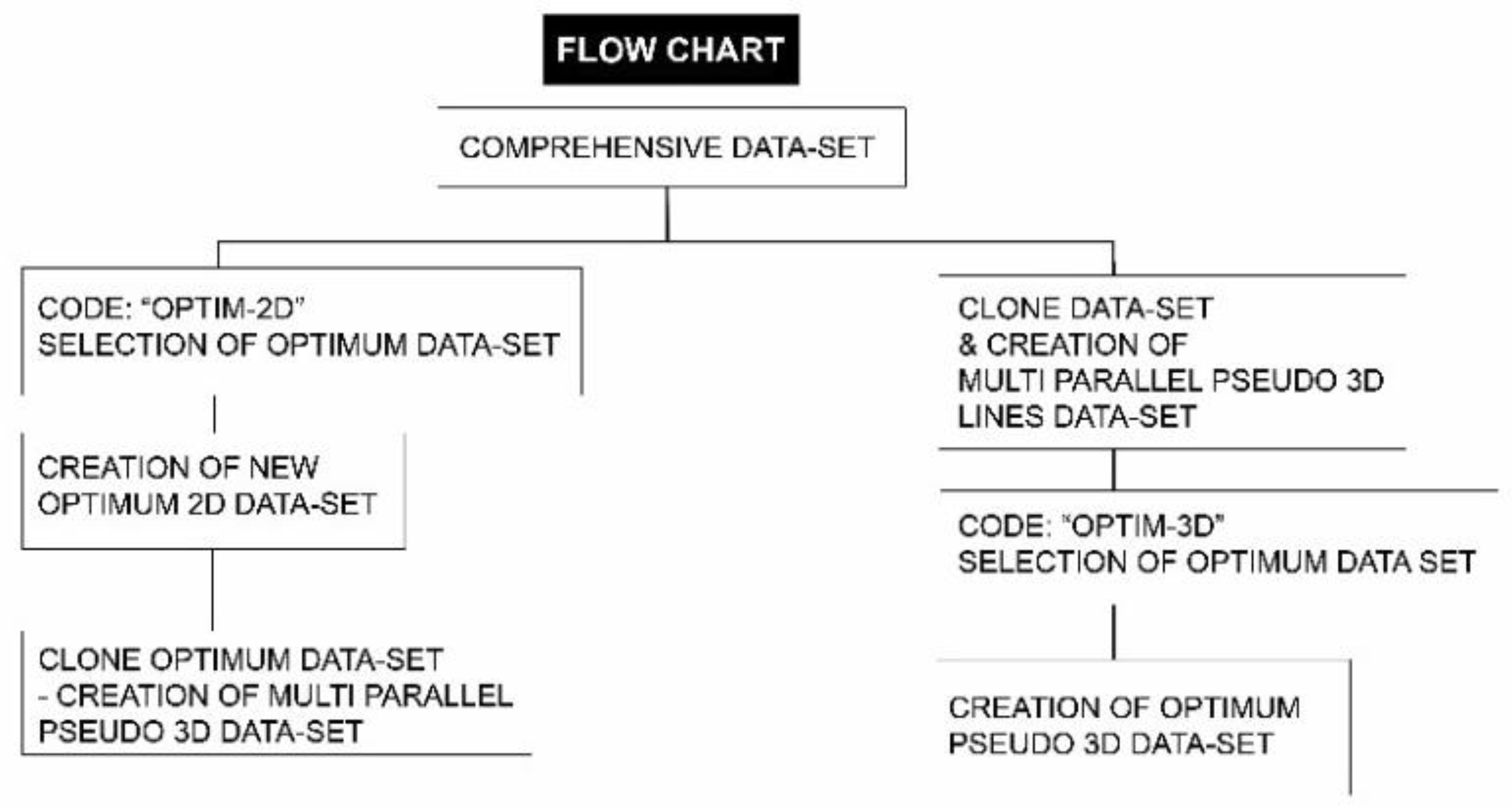
A demonstrative way of producing the 3-D optimum measurements from the comprehensive data set is shown in Figure 3. From the initial comprehensive (normal) 2-D tomographic data set (Figure 3, red-colored profile view), the 2-D algorithm is used to select the optimum data for a single 2-D profile (Figure 3, green-colored). Then, this optimum 2-D data set is cloned in multiple parallel profiles equally separated to create the 3-D optimum data set.

On the other hand, for the 3-D optimization technique, the initial comprehensive 2-D data are firstly cloned in multiple equally separated parallel profiles (Figure 3, red-colored) and then the 3-D algorithm produces the 3-D optimum data (Figure 3, blue-colored). In the present study, both 2-D and 3-D optimization algorithms were allowed to run for specific steps to maintain equal measurements for the ‘Optim-2D’ and ‘Optim-3D’ protocols, respectively, for direct comparison purposes.

Table 1. Number of data for FULL protocol (percentage of initial array).

Protocol	a	na	Comprehensive	Optim-2D	Optim-3D	Stummer’s
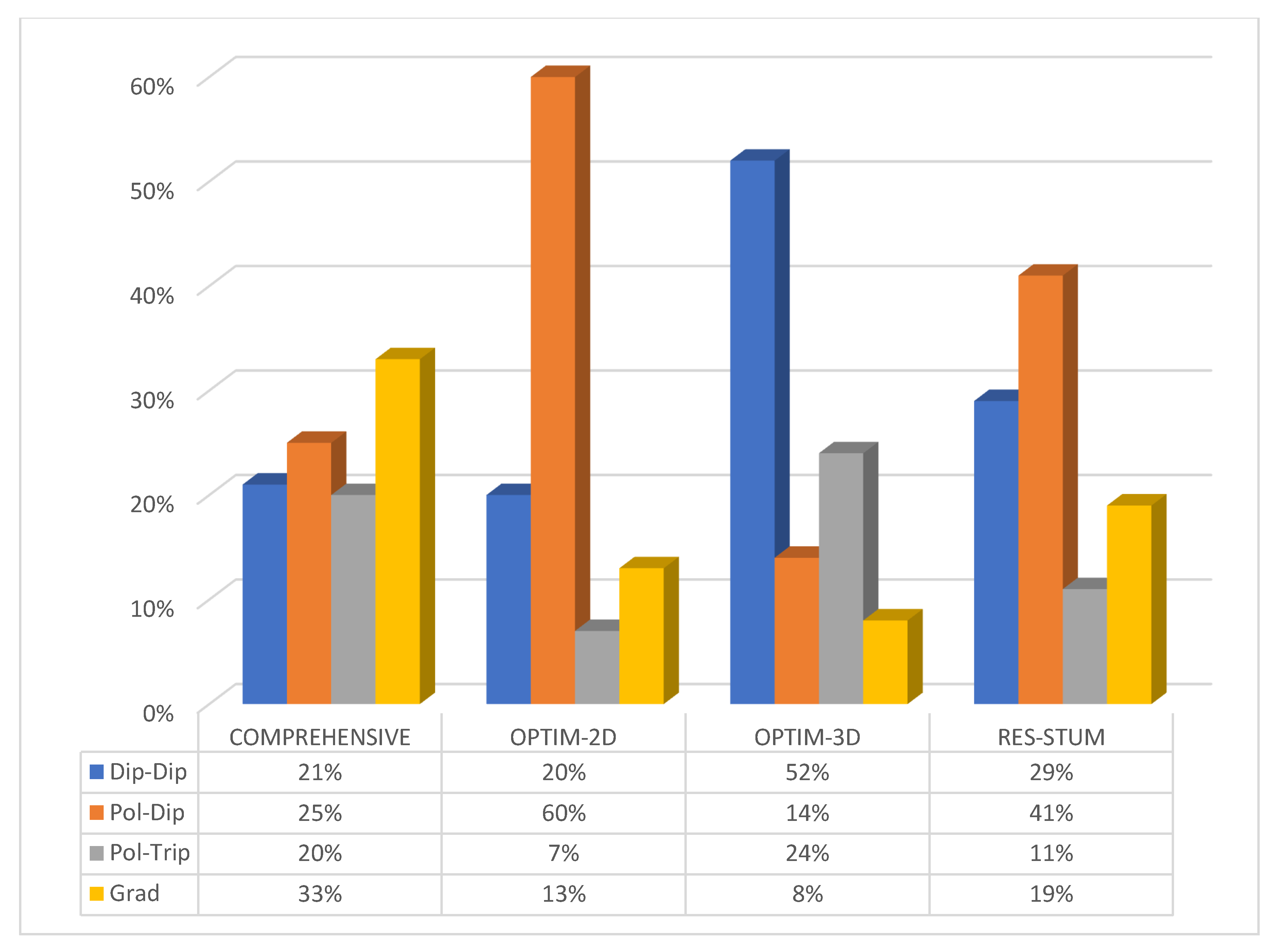
FULL	1–9	17	23,670 (100%)	3390 (14%)	3315 (14%)	5224 (22%)

shows the unit electrode spacing ‘a’ and the separation factor ‘n’ used to compile the 23,670 measurements of the comprehensive data set, comprised of dipole–dipole (DD), pole–dipole (PD), pole–tripole (PT) and gradient (GR) array, assuming 11 parallel profiles. The final resulted in “Optim-2D” and “Optim-3D” protocols each being only 14% of the initial comprehensive data set. The “Res-STUM” protocol used only 22% of the initial comprehensive data set. Figure 4 shows the percentage participation of each protocol that was used. A comparable quantitative analysis of the resolving capabilities of the different protocols based on the cumulative Jacobian values per parameter is shown in Figure 5. The cumulative values have been normalized according to the total number of the data to gain the flexibility of comparing protocols with uneven measurements. As is expected, higher sensitivity values are the ones closer to the surface. The normalized cumulative Jacobian of the “optim-3D’ data set has higher values than the “optim-2D”. Furthermore, the sensitivity pattern of the “optim-3D” is more intense in the deeper layers, thus indicating a higher capability in resolving deeper resistivity structures.

3. Synthetic Model

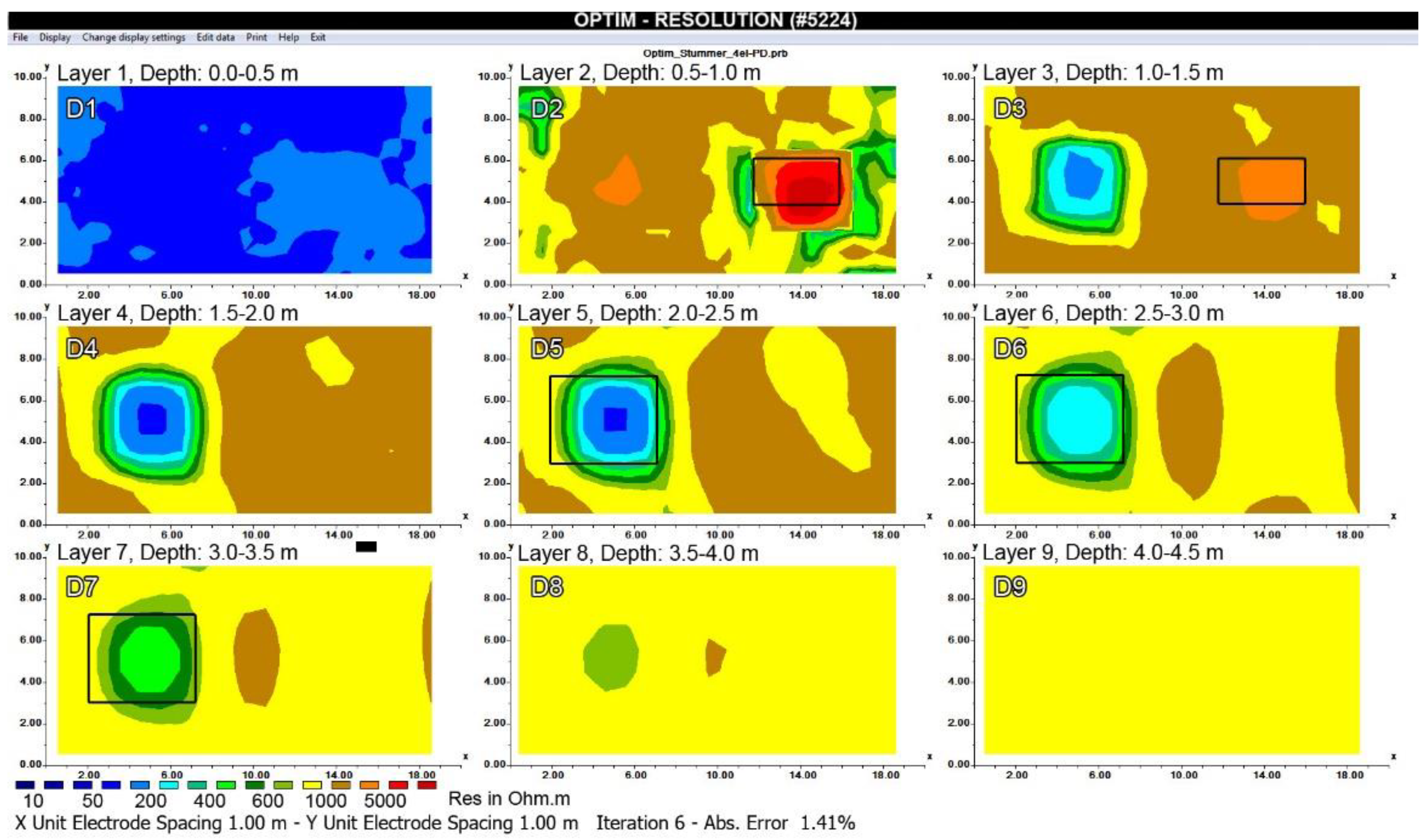
The efficiency of the optimization algorithm was firstly tested with synthetic data in order to evaluate the resolving capabilities of the generated optimized protocols under constrained conditions, where the exact targets’ position and resistivity values are predefined and well-known. The resistivity model used in the work of Stummer et al. [15] was extended in the 3-D space, composed of nine layers (D1–D9) with a constant thickness of 0.5 m (Figure 6). A homogeneous half-space of 1000 ohm.m lies below a less resistive superficial layer of 100 ohm.m one meter thick. A highly resistive target ‘A’ (3 × 2 × 1 m) with a resistivity of 10,000 ohm.m is buried at 0.5 m from the ground surface lying within the two horizontal layers D2–D3. A target ‘B’ with larger dimensions (5 × 4 × 1.5 m) is buried at 2 m depth from the surface within the layers D5 to D7. The resistivity of this block gradually decreases inwards from 100 to 10 ohm.m.

The 3-D resistivity survey was composed of total 231 electrodes in total arranged in a rectangular grid of 20 m by 10 m along the X and Y axes, respectively. The inter-probe and inter-line spacing were set to 1 m on both axes. The tomographic data were collected along the 2-D profiles on the X-axis using the combination of the four traditional arrays (dd + pd + pt + gr) and the measuring parameters shown in Table 1. A 3-D finite element algorithm (RES3DMOD) was used to calculate the forward response of the specific model and extract the distribution of the apparent resistivity values for the comprehensive data in the 3-D subsurface space. The synthetic apparent resistivity data were then corrupted with 5% Gaussian noise on the modeled apparent resistivity values.

During the inversion procedure, the L1-norm method was used for data misfit and model roughness to account for the sharp boundaries of the targets [30]. A finite-element modelling subroutine was used to calculate the apparent resistivity values. The selected initial value for the damping factor was λ = 0.1, which was increasing with a depth factor of 1.01. The inversion procedure was terminated after five iterations. The common resistivity colored scale (10–10,000 ohm.m) and depth slices (D1–D9) are used in all inversion images for comparison purposes. Black squared rectangles indicate the expected exact position of targets ‘A’ and ‘B’. The RMS error value varies between 3.7 and 4.1% among all the inversion images of the arrays that were used.

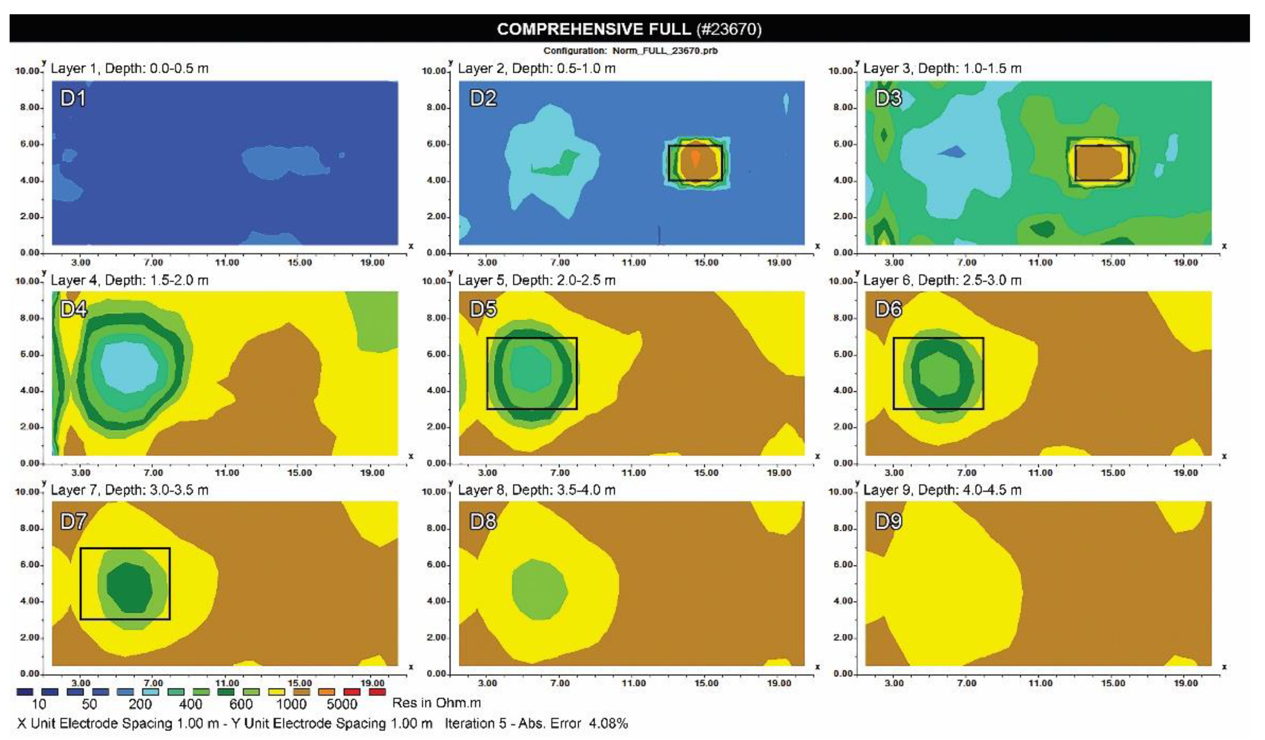
The comprehensive FULL protocol (Figure 7) reconstructs the targets ‘A’ and ‘B’ with comparable accuracy: the calculated resistivity value for target ‘A’ is approximately 1000 ohm.m. It is located inside the rectangular lines and the corresponding depth slices (D2 and D3). The target’s ‘B’ resistivity value is close to 500 ohm.m. The target’s location at the XY axis is well located but not on the Z-axis, where it is extended to layer depth D4.

The Optim-2D data set (Figure 8) is able to reconstruct the target’s ‘A’ position inside the rectangular box but the resistivity value (500–1000 ohm.m) is lower than the comprehensive data set value. The target ‘B’ is also located inside the expected rectangular area with resistivity values that vary between 400–600 ohm.m and it is expanded at depth D4.

The higher and closer to true value resistivity value of 5000 ohm.m is presented with the Optim-3D data set regarding the reconstruction of target ‘A’ (Figure 9). Additionally, the position of target ‘A’ is inside the expected position. Target ‘B’ is reconstructed with a small shift downwards along the XY direction. The resistivity value varies between 400 and 500 ohm.m. Similarly, as noticed before, target ‘B’ is shifted downwards at depth level D4.

Stummer’s optimum data reconstruct target ‘A’ only at layer D2 (not at D3) with higher resistivity values (>5000 ohm.m) and deformed along the Y direction (Figure 10). The layer D2 is reconstructed with values close to 1000 ohm.m, a value higher than the model (100 ohm.m). Target ‘B’ is also reconstructed at depth layers D3 and D4, where it should not be, but with resistivity values closer to the theoretical model (100 ohm.m).

It should be noted that both optimum data sets (Optim-2D, Optim-3D) are able to reconstruct the target’s position while using only 14% of the initial comprehensive data set. Furthermore, the Optim-3D data set shows comparable accuracy regarding the target’s resistivity value among all the other data set (comprehensive and Optim-2D) but the location of target ‘B’ was shifted slightly away from the expected location. All data sets reconstructed target ‘B’ at depth level D4 due to the smoothness constraints imposed in the inversion to stabilize the inversion.

4. Quantitative Analysis

The quantitative comparative analysis between the resistivity models resulting in the inversion of the comprehensive and optimum data sets was made feasible using the model misfit and the layer RMS. The above-mentioned techniques were used to validate the degree of model matching on the inverted model with respect to the true model as predefined by the initial user resistivity values. The model misfit is defined as the mean squared misfit between the true parameter model ρ_t and the inverted parameter model ρ_c resistivity value [27]:

$$Model Misfit={\left(\frac{1}{N}{\displaystyle \sum }_{i=1}^N{\left[log\left({\rho }_t\left(i\right)\right)-log\left({\rho }_c\left(i\right)\right)\right]}^2\right)}^{0.5}{}^{}$$

(1)

The layer RMS is the root mean square error for each layer defined as the percentage difference in the resistivity values between the true and the inverted model using the following equation [31]:

$$layer RMS=\sqrt{\frac{1}{N}{\displaystyle \sum }_{i=1}^N{\left(\frac{{\rho }_c\left(i\right)-{\rho }_t{\left(i\right)}_{}}{{\rho }_t\left(i\right)}\times 100\right)}^2}$$

(2)

The results of the calculations are shown in Figure 11. All values (model misfit and layer-RMS) are calculated for the FULL array only for five specific depth model layers (D2, D3, D5, D6 and D7) where the targets exist. The model misfit values of the Optim-3D data set (green-colored line) are profoundly decreased at the superficial depths (D2, D3) then equalize with the comprehensive and Optim-2D data sets at deeper levels (D5, D6, D7). The Optim-2D data set (yellow-colored line) has a higher value of model misfit at depth D2 from the Optim-3D data set and equal value with the comprehensive data set. At depth of D3, the Optim-2D data sets have lower model misfit values in comparison with the comprehensive data set and higher value in comparison with the Optim-3D data set. For the following depths (D5, D6, D7), the Optim-2D data set shares the same model misfit values with Optim-3D and comprehensive data set.

Regarding the layer-RMS values, the comprehensive data sets (red-colored line) share the same values with the optimum data sets (Optim-2D, Optim-3D) at superficial depth layers (D2, D3, D5). For deeper layer D6, the layer-RMS value of optimum data sets is higher than the comprehensive data set: Optim-2D data set has the highest value in comparison with the Optim-3D and the comprehensive data set. At the deepest layer D7, comprehensive, Optim-2D and Optim-3D share the same layer-RMS value.

The Res-STUM data (blue-colored line) presents a high value model misfit and layer-RMS at depth layer D2 showing a decreased efficiency of the optimized protocols to reconstruct the shallow depth layers. On the other hand, it seems to have lower values than the comprehensive data set, Optim-2D and Oprim-3D approaches at deeper depth layers.

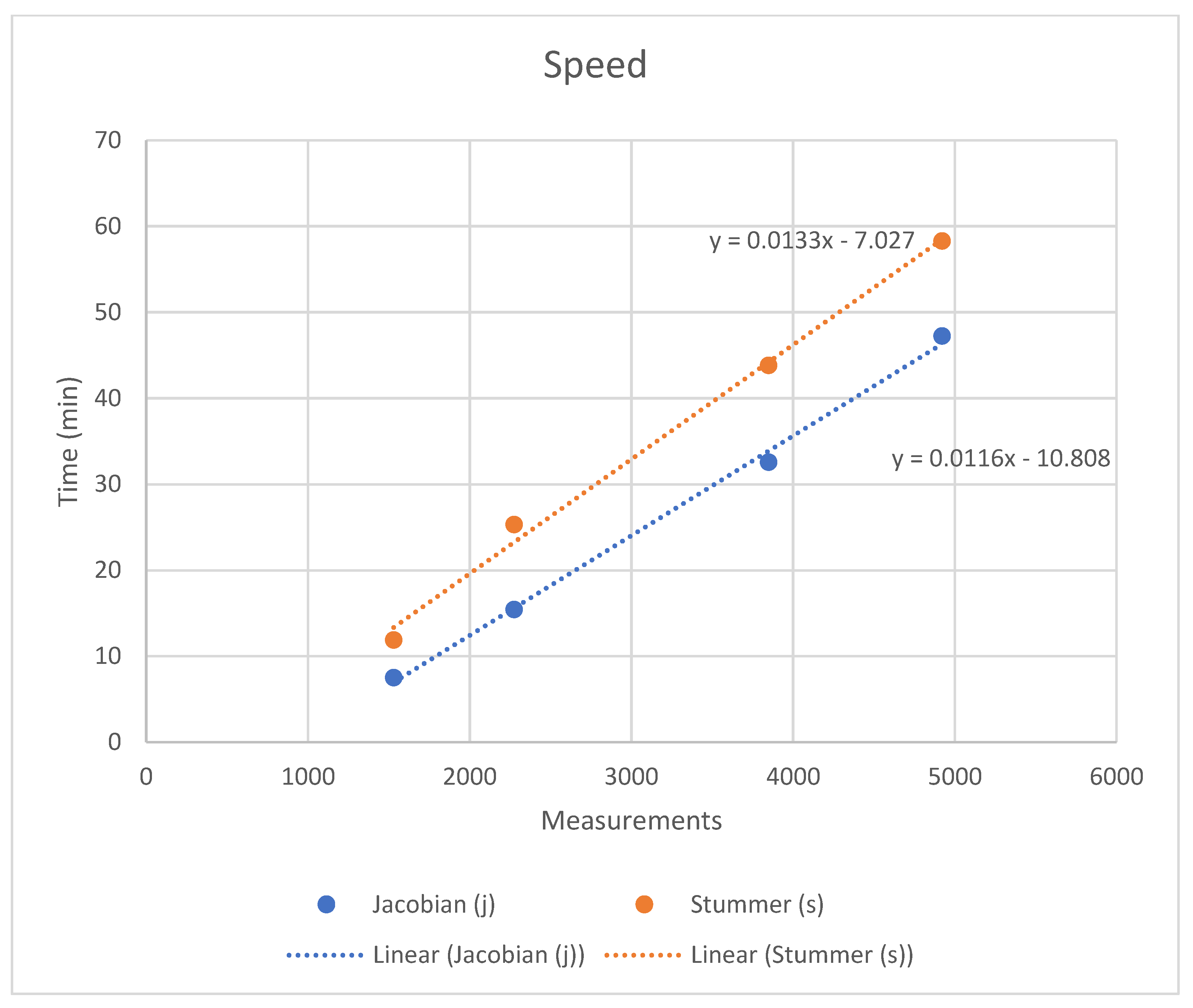
The time to compute the 3-D optimized protocols with both the Jacobian and the Stummer’s method will depend on the number of electrodes, the size of the comprehensive data set and the scheme to parametrize the subsurface in homogeneous 3-D resistivity blocks. Assuming a 3-D ERT survey where the number of electrodes and the parameters is fixed, the total time to extract the optimized data sets with the two algorithms will depend on the size of the comprehensive data set. Both algorithms seem to have a linear increasing trend relating the time and the number of measurements. However, the Jacobian method shows a relative reduction of more than 20% in the actual time needed to compile the optimized data sets, thus being significantly faster than Stummer’s approach (Figure 12).

5. Field Data

5.1. Panormos (Rethymno)

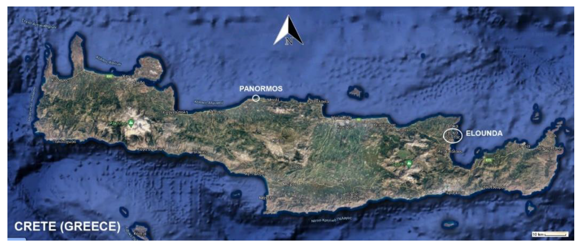
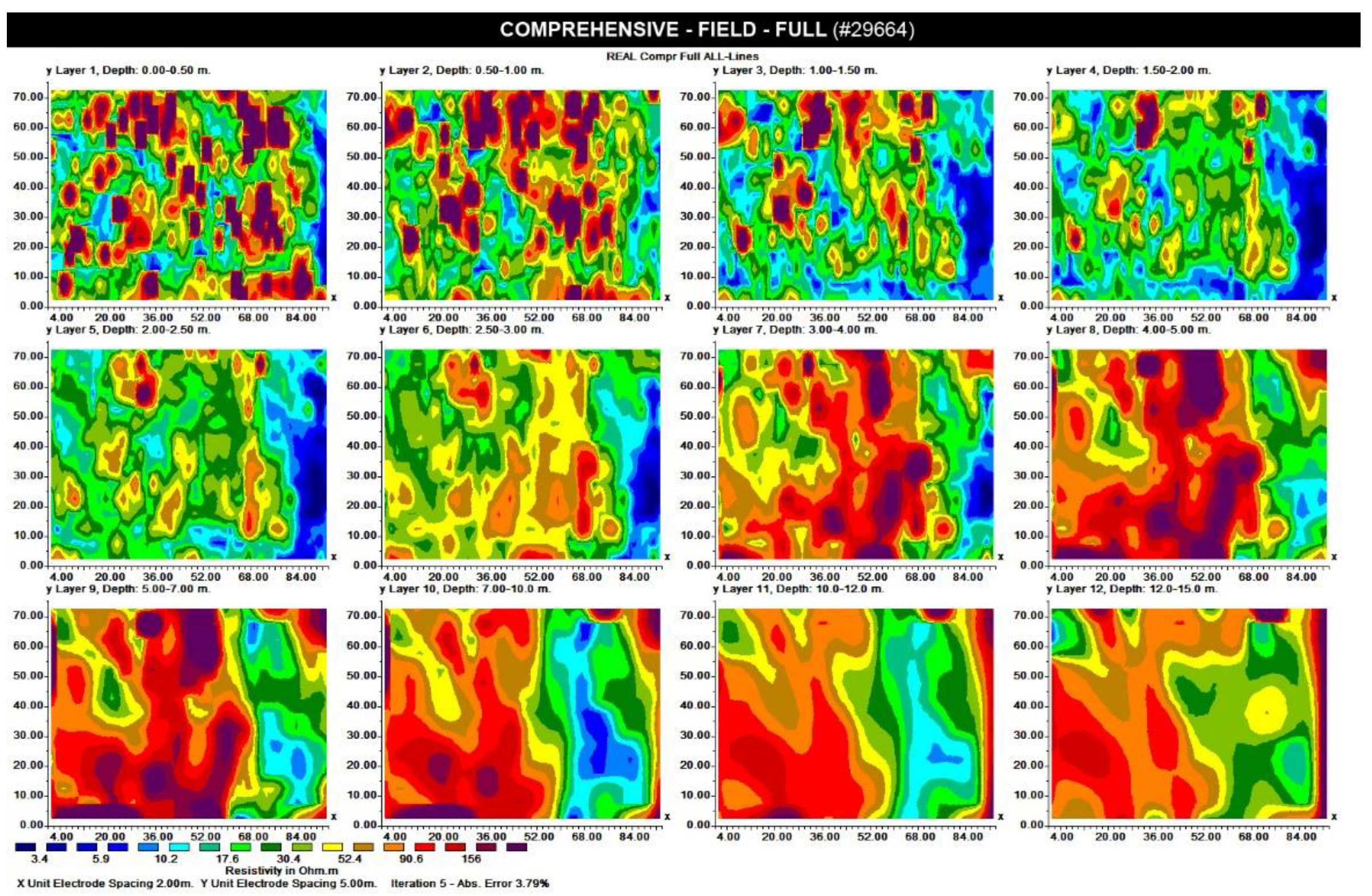
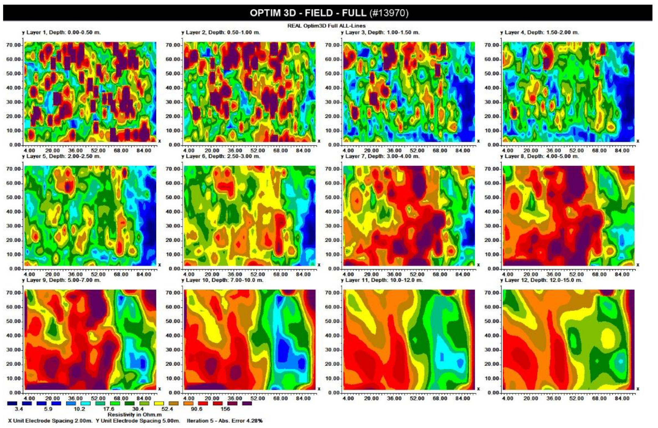
The field data were collected for a geotechnical study at the city of Panormos, east of Rethymno (Crete, Greece) (Figure 13). The selected grid was 94 × 75 m, where 16 parallel survey lines (5 m apart) were used to collect the geoelectrical data. For each line, 48 electrodes were used with 2 m probe spacing. Each line collected 1216 (dipole–dipole) and 638 (gradient) data, producing an overall complete data set of 19,456 dipole–dipole and 10,208 gradient data in total from the 16 lines. All data were used to produce the comprehensive FULL data set (dd + gr), which consists of 29,664 measurements.

The final Optim-2D optimized data set that was created by the 2D optimization procedure selected 15,214 measurements (10,035 dd and 5179 gr). The Optim-3D data set with 13,970 measurements were created from the 3-D optimization procedure which selected 8658 dipole–dipole and 5312 gradient data. The amount of optimum data that was selected from the 2-D and 3-D algorithms from the comprehensive data set is 51% and 47%, respectively. The Res-STUM optimum data set used 14,943 measurements (50%). All data were inverted with the same inversion parameters and are presented with a common resistivity scale from 3.4 to 205 ohm.m. The estimated RMS error for all inversion models is ranged from 3.0 to 3.87% after five or six iterations. The deepest depth layer reaches 15.0 m below the ground (Figure 14, Figure 15, Figure 16 and Figure 17).

Based on the geoelectrical model in the research area, a surface layer of about 2.5 to 3.3 m thick is detected with resistivity values from 20 to 70 ohm.m. This layer coincides with the topsoil and the recent surface deposits. Within this layer, there are areas of increased resistivity values due to local concentrations of rock masses, resulting from the disintegration of the rocky background.

From the depth of 3.3 m up to the maximum depth of the geophysical survey (15 m), a formation with high resistivity values over than 70 ohm.m) appears, which is associated with the rocky background of the slates and shale in the wider area. The rocky background entirely covers the western area and extends east to a horizontal distance of 60 m. It also appears that the rocky background is not continuous and exhibits an intrinsic heterogeneity, as can be observed from changes in resistivity within the same formation. This means that the rock is fractured internally, mainly at sections where lower resistivity values are registered. Such an area is located on the northwest side of the area (X = 0–26 m and Y = 35–75 m) where it appears with resistivity values in the range of 30 to 40 ohm.m.

The most characteristic geophysical anomaly is the area to the eastern side, which appears with very low resistivity values below 20 ohm.m. This zone is superficial and appears to continue at the deeper slices. This area seems to lean westward and is bound west and east by the rocky background. To the east, this rocky background appears with high resistivity values mainly from the depth of 7 m.

The above range of low resistivity values can either be connected to a paleo-river due to the conductive signature of the sediments because of the water flowing in them. This area may also have originated from a local fragment of the rocky background so that, again, the water has the ability to move freely in this area and affect the values of resistivity.

The inversion results show a comparable accuracy among the resistivity models reconstructed by the inversion of the comprehensive, optim-2D, optim-3D and Res-STUM data sets: the mapping of the bedrock, which was the main interest of the study, is reconstructed at the same position and depth slices of both comprehensive and optimum inversion results.

5.2. Elounda (Agios Nikolaos)

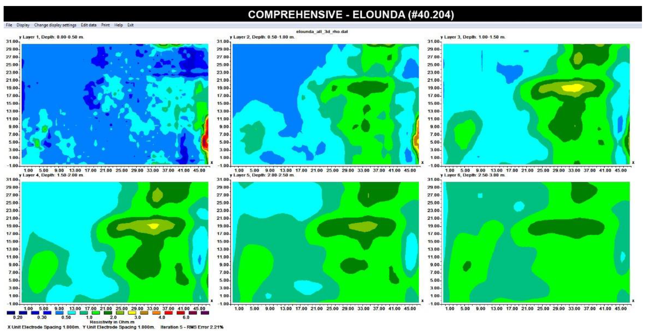
The field data were collected from the bay of Elounta (Crete, Greece). The selected grid was 30 × 47 m where 31 parallel survey lines (1 m apart) were used to collect the geoelectrical data in the marine environment. For each line, 48 submerged electrodes were used with 1 m probe spacing in depth varying from 0.07 m to 2.86 m and the resistivity of water was measured 0.2 ohm.m. Each line collected 1298 (pole–dipole forward and reverse), producing an overall complete data set of 40,204. All data were used to produce the comprehensive FULL data set.

The Optim-3D data set with 21,184 measurements were created from the 3-D Jacobian optimization procedure. The amount of optimum data that was selected from 3-D algorithm from the comprehensive data set was 50%. All data were inverted with the same inversion parameters and are presented with a common resistivity scale from 0.2 to 7 ohm.m. The estimated RMS error for all inversion models is from 1.56 to 2.21% after five iterations. The deepest depth layer reaches 3.0 m.

Both models (Figure 18 and Figure 19) present similar results revealing a linear resistive area which extends from the depth of 0.5 m up to 2.5 m located between 23 and 38 m in the x direction and 18 to 21 m in the y direction. This area is correlated with the visible archaeological remains of a possible wall or tower. The relatively resistive area that extends from 29 to 41 m in the x direction across the y direction could be related to collapse parts of the aforementioned structure or with a poorly preserved wall. The area (0–25 m in x, 0–30 m in y) is dominated by the conductive sandy seafloor. A resistive target (1–7 m in x, 3–11 m in y) inside that area could be either beach rock, also visible in other parts of the bay, or some other archaeological relics.

6. Conclusions

The work describes an experimental method to select electrode configurations that carry the maximum resolving capability in order to reconstruct the subsurface resistivity distribution. The technique is based on the sensitivity and the examination of Jacobian matrix entries. The basic differences of the specific method in relation to approaches utilizing the model resolution matrix to select the optimum array protocols have already been stressed for the 2-D resistivity problem. The main one is attributed to the fact that the optimum data set is created solely depending on each individual array. On the contrary, the initiation of any algorithm based on resolution matrix approaches needs the compilation of an initial base data set and the enrichment of this base set with added configurations coming from a comprehensive data set having every possible electrode combination based on the update of the resolution matrix. Thus, the sensitivity approach can be faster since the calculation of the Jacobian is part of the forward resistivity problem and there is no need to perform any inversion, as is the case for the resolution matrix approaches. The comparative tests performed in this work showed that the Jacobian method is about 20% faster than previous approaches using the resolution matrix. Furthermore, the Jacobian matrix method avoids the evaluation of the goodness function since the algorithm picks the most sensitive measurements. Therefore, the extra time gained in selecting optimum measurements is increased, which is amplified in cases of large 3-D resistivity tomographic problems and data.

The 3-D optimum protocols are produced from 3-D data sets compiled by the merging of multiple equally spaced parallel 2-D profiles assuming traditional arrays: dipole–dipole, pole–dipole, pole–tripole and gradient. The two different approaches involved the application of 2-D and 3-D optimization algorithms to select the optimum protocols ranged from 14% (synthetic data set) and ~50% (field data set) of the original full data sets. The cumulative Jacobian matrix (normalized sensitivity value of each parameter) showed that the optimum protocols have the same sensitivity values with the full data set, although fewer measurements are used than the traditional protocols.

The algorithms were validated with a synthetic model where the inversion results verified the comparable similarity of the reconstructed models between the comprehensive and the optimum (from 2-D or 3-D) data sets. The efficiency of optimization procedure was validated with field data from completely different environments using a comprehensive data set which is comprised of different traditional arrays (dipole–dipole and gradient, pole–dipole forward and reverse), where the inversion models of the optimum protocols showed similar results, although half of the initial complete data set was used for the inversion.

In general, the specific work shows the flexibility and effectiveness of an experimental procedure based on the sensitivity matrix in selecting optimum resistivity protocols in a 3-D context. The two different approaches in compiling the optimum 3-D tomographic protocols show comparable results in terms of the inverted resistivity models. In relatively more complicated subsurface geometry and resistivity distribution, the full 3-D optimization method can give slightly superior results in relation to the 2-D approach with minimum extra time. Finally, the optimized data sets can also be used as a basis for 3-D monitoring experiments to experience enhanced resolving capabilities of the time-lapse resistivity images for monitoring the subsurface contamination in environmental applications [32].