Article

Safe Vehicle Trajectory Planning in an Autonomous Decision Support Framework for Emergency Situations

COSYS-PICS-L, University Gustave Eiffel, 77202 Marne la Vallée, France
*
Author to whom correspondence should be addressed.
Current address: 25 Allée des Marronniers, 78000 Versailles, France.
Appl. Sci. 2021, 11(14), 6373; https://doi.org/10.3390/app11146373
Submission received: 25 May 2021 / Revised: 29 June 2021 / Accepted: 5 July 2021 / Published: 9 July 2021
(This article belongs to the Special Issue Human-Computer Interaction: Theory and Practice)

Abstract

:
For a decade, researchers have focused on the development and deployment of road automated mobility. In the development of autonomous driving embedded systems, several stages are required. The first one deals with the perception layers. The second one is dedicated to the risk assessment, the decision and strategy layers and the optimal trajectory planning. The last stage addresses the vehicle control/command. This paper proposes an efficient solution to the second stage and improves a virtual Cooperative Pilot (Co-Pilot) already proposed in 2012. This paper thus introduces a trajectory planning algorithm for automated vehicles (AV), specifically designed for emergency situations and based on the Autonomous Decision-Support Framework (ADSF) of the EU project Trustonomy. This algorithm is an extended version of Elastic Band (EB) with no fixed final position. A set of trajectory nodes is iteratively deduced from obstacles and constraints, thus providing flexibility, fast computation, and physical realism. After introducing the project framework for risk management and the general concept of ADSF, the emergency algorithm is presented and tested under Matlab software. Finally, the Decision-Support framework is implemented under RTMaps software and demonstrated within Pro-SiVIC, a realistic 3D simulation environment. Both the previous virtual Co-Pilot and the new emergency algorithm are combined and used in a near-accident situation and shown in different risky scenarios.

1. Introduction

In the last 20 years, the transportation paradigm has evolved in order to improve road safety, minimize energy consumption and pollutants emissions, and optimize traffic conditions [1,2]. One of the key solutions is the development and deployment of automated mobility (level 3 to 5 of SAE (Society of Automotive Engineers) standard). With the expected functionalities of such automated systems, the mobility concepts will strongly and radically evolve. Technologies are a crucial issue in the development of this new generation of mobility means. Technology issues are not only focused on new powertrains, new hardware architecture, or new types of efficient embedded sensors for Autonomous Driving Systems (ADS) (i.e., radar [3], lidar, IR-neuromorphic-UHD-Polarized-Stereo-Fisheye cameras, GPS [4], etc.) but also on new methods, approaches and algorithms in order to process the data coming from information sources (sensors, HD Maps, communication). Artificial Intelligence (AI) takes an increasingly important role in the “onboard intelligence” [5]. Thus, sensors provide information to the perception layer which allows to assess the attributes of the road key components (obstacles, road, ego-vehicle, environment, and driver). This perception information allows building dynamic local perception maps, which can then be extended by sharing data using specific Vehicle to Vehicle or Vehicle to Infrastructure communication protocols. From these maps, decision module and path planning methods can be implemented in order to drive vehicles automatically and safely without any human active operation (see Figure 1).
In a fully autonomous driving system, while perception modules are compared to human eyes and ears, decision-making and planning are the “brains” of autonomous driving, control/command stages being the feet and hands. In this architecture, the decision-making and planning modules represent the system’s intelligence (reasoning layer). Like for human operating, after the brain receives various stimuli and perception information, the decision layer analyzes them to understand the current environment and then apply strategies to move according to constraints (safety, energy, comfort, etc.). Then, the decision-making module generates instructions (path, trajectory, orders, maneuvers, or advice) to the control module. The level of complexity that a decision-making planning module can handle is a core indicator for measuring and evaluating autonomous driving capabilities [6]. Another indicator is its ability to respond to unexpected events by rapidly re-planning its trajectory.

1.1. Problem Description

In a very general setting, path planning refers to finding a continuous mapping σ : [ 0 , 1 ] X (a path), in a given environment with known boundaries and obstacles embedded in a state-space X. Constraints on this mapping typically include:
  • Constraints on the initial state σ ( 0 ) (position, orientation, etc.) and the final state σ ( 1 ) (location of the target point);
  • Staying within the boundaries and avoiding collisions with obstacles σ ( α ) X f r e e , α [ 0 , 1 ] ;
  • Geometric constraints on the path, typically a maximum curvature.
However, when moving obstacles are taken into account, a simple path planning algorithm (i.e., generation of a geometric path between the origin and the destination) cannot be used alone, and the time dimension must be added. In this case, the planning problem can not be solved in polynomial time, and becomes an NP-hard problem [7]. Correspondingly, the constraints change to:
  • Constraints on the initial state and the sub-goal state, considering the time dimension.
  • Constraints on staying within the boundaries and avoiding moving obstacles;
  • Differential constraints on the trajectory, typically upper bounds for speed, acceleration, steering, and steering rate.
This problem is now called trajectory planning. It can be broken down by using a “path-speed” decomposition approach, where the geometric path and the speed profile are computed separately, but this is not always possible or optimal. These real-time planning algorithms typically run continuously with a receding horizon, and must be robust enough to handle sudden changes in their environment. In simulation, these emergency situations can be used to test the algorithm’s limits.

1.2. Literature Review

1.2.1. Decision Making

Different decision-support architectures have been applied to autonomous driving. In a controlled environment (such as in the 2007 DARPA Urban Challenge [8]), rule-based [9,10] and knowledge-based [11,12,13] methods have been successfully applied. However, these methods assume full knowledge of the traffic environment, including the other road users intent. Considering the uncertainty in the environment, the tactical decision task is usually modelled as a Partially Observable Markov Decision Process [14], which has been applied to different driving scenarios [15,16,17]. The core of the planning-based method is trajectory planning, i.e., generating a trajectory for a given scenario [18,19,20] based on the trajectories of other vehicles, but its applicability is still limited in a highly interactive environment. The rapid development of machine learning allowed using learning-based methods for autonomous driving decision-making in highly interactive environments, such as the imitation learning method [21,22], or more recently a combination between traditional methods and reinforcement learning methods [23].

1.2.2. Path and Trajectory Planning Algorithm

Solving the lower dimensional planning problem through the search space is a common approach for path planning. The basic idea is to discretize the state space into a graph and then use a search algorithm such as Dijkstra [24] or A* [25] to find feasible solutions or optimal solutions. The A* algorithm is an extension of Dijkstra, which assigns weights to nodes based on a heuristic-estimated cost, then performs a fast graph search to the target node. Many different variations based on this algorithm have been proposed for path planning: Hybrid A* [26], Theta* [27], Filed D* [28], D* Lite [29], etc. Besides, several planning approaches [30,31] have been proposed to increase the system reliability, considering the localization uncertainty problem.
However, when it comes to the trajectory planning problem in a dynamic and continuous environment, the search space dimensions will increase, leading to significant computational time growth. In this case, the planning problem can be approximated to a discrete sequence of optimization problems by sampling the continuous state space. The representative algorithms are Probabilistic Road Map [32], and Rapidly-Exploring Random Tree (RRT) [33] algorithms, which have a good performance in high-dimensional non-convex state spaces. The latter method has been extensively adopted in the trajectory planning for autonomous driving [34,35], with several improvements to the RRT algorithm being proposed over the years, either to reduce the computation cost (anytime RRT [36], RRT-Connect [37], and Dynamic RRT [38], etc.), or to optimize the generated path (RRT* [39,40]).
When faced with the trajectory planning problem in a dynamic and continuous driving environment, Artificial Potential Field (APF) methods [41] use a continuous equation, similar to the electrostatic potential field. APF methods can easily be implemented and executed in real-time for control and navigation [42]. In these algorithms, the moving object tries to reach a target and to avoid obstacles on the trajectory by using virtual forces that either attracts it or pushes it away. One benefit of this framework is that different constraints can be taken into account by simply adding specific forces, and several new potentials have been proposed, based on the road structure (with lane and boundary potentials) or on vehicle physics (guided potential), in order to use APFs in different scenarios of autonomous driving (highway [43], intersection [44]). Several improvements were proposed to solve different limitations [45] of the traditional APF algorithm for autonomous driving. An improved APF model [46] was designed to avoid the local minimum problem, which can also be tackled by using a virtual obstacle [47], or a virtual target point [48]. By modifying the calculation of APF using fuzzy logic, the nearby obstacle problem can be dealt with. In [49], an additional artificial friction force was introduced to limit oscillations. Although APF algorithms can provide adequate trajectories as the results, the final configuration of the vehicle is unpredictable, which may lead to dangerous situations. Another general problem with this method is that the kinematic constraints of the vehicle are very difficult to take into account, thus the mechanical feasibility of the trajectories cannot be guaranteed.
Elastic bands (EB) methods [50] also come from a physical analogy. In these methods, the planned path of the object is simulated through a series of springs that can be deformed to react to changes in the environment. Refs. [51,52] applied EB theory to the emergency path planning problem. Song [53,54] proposed specific forces to respect different constraints, such as the lane constraint, to make the vehicle drive on a given lane, and the guide-potential constraint, to avoid collisions between following vehicles. The internal forces of the EB provide a constraint to neighbouring trajectory nodes, but the method still struggles with precise kinematic constraints. Choosing the trajectory’s final point (during re-planning) is also an difficult issue in emergency situations.

1.2.3. Vehicle Control

The role of vehicle control in the autonomous driving architecture is to track the theoretical trajectory computed by the planning algorithm. Models of vehicle kinematics, like the bicycle model [55], are used to translate this trajectory ( x ( t ) , y ( t ) ) into a series of commands, usually steering angle and acceleration. Different controllers have been used for autonomous driving at relatively low speed: Proportional Integral Derivative (PID) controllers [56], pure pursuit controllers [57], Stanley controllers [58], among others. Dynamic model-based control methods have better performance at high vehicle speed or with a large curvature change rate. Nonlinear control [59], Model Predictive Control (MPC) implementations [60,61,62] and feedback-feedforward control [63] can increase the stability of the vehicle at high speeds.

1.3. Contribution

This paper looks to improve a planning algorithm developed at Eiffel University [64] by testing its limits in emergency situations. The main contributions of this paper, developed for the EU H2020 Trustonomy project [65], are the following.
  • A general decision-support framework for autonomous driving is introduced, which uses a combination of two different algorithms for trajectory planning (“autonomous mode” and “emergency mode” algorithms). This expanded framework keeps the efficiency of the previous algorithm but improves its robustness in emergency situation.
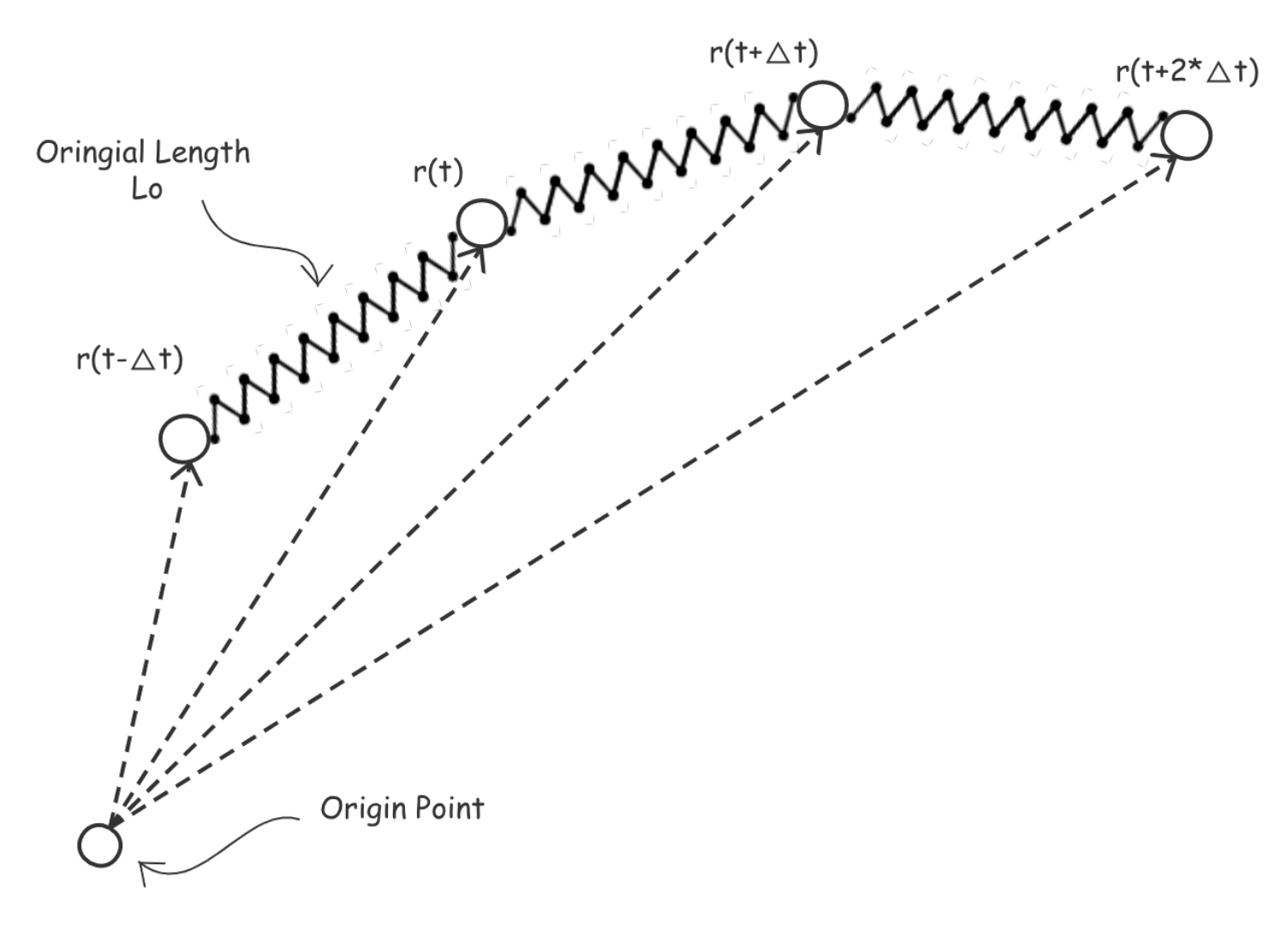
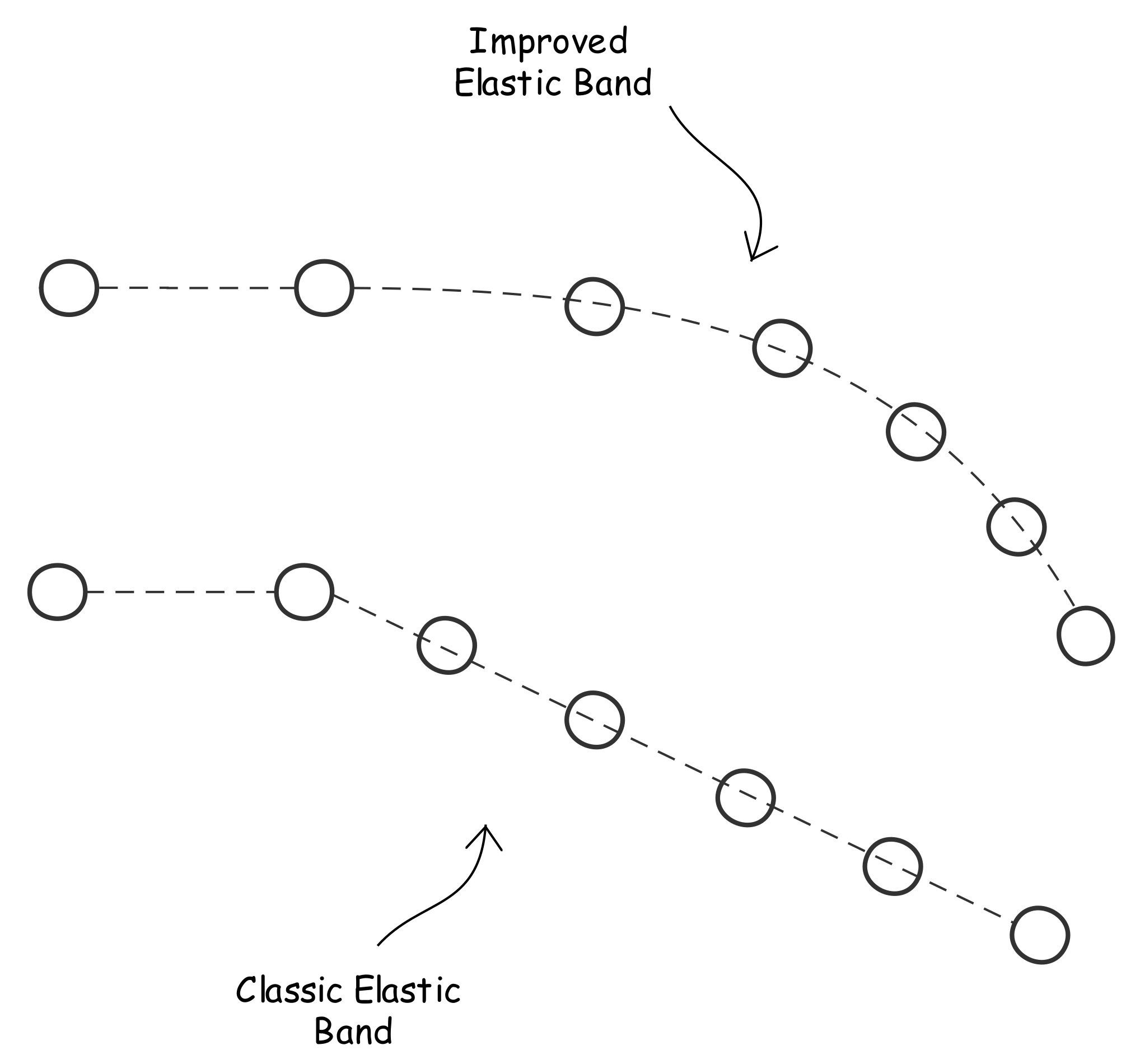
  • An emergency trajectory planning algorithm was developed, based on elastic bands. The following improvements are presented:
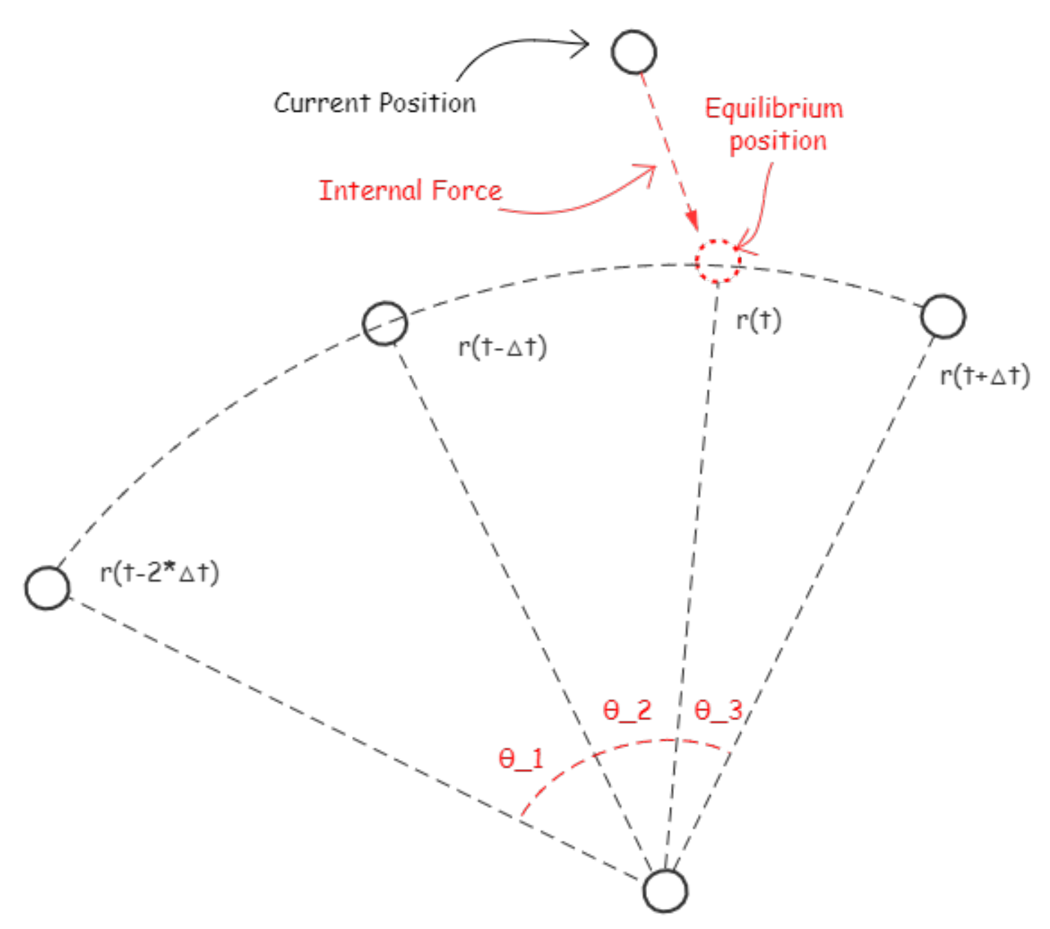
    A new internal force is proposed, to ensure the steering and acceleration of the vehicle stay bounded (kinematic constraints);
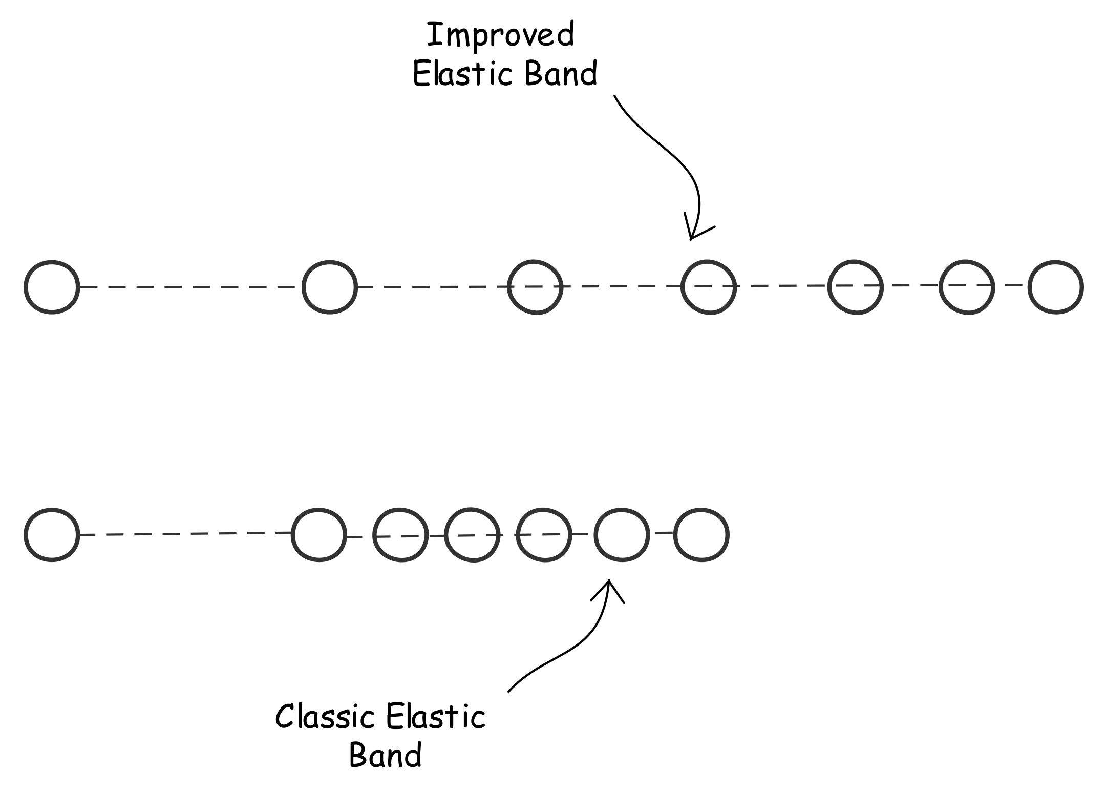
    The last point of the trajectory is not fixed, but instead is subject to specific internal and external forces, to give more flexibility;
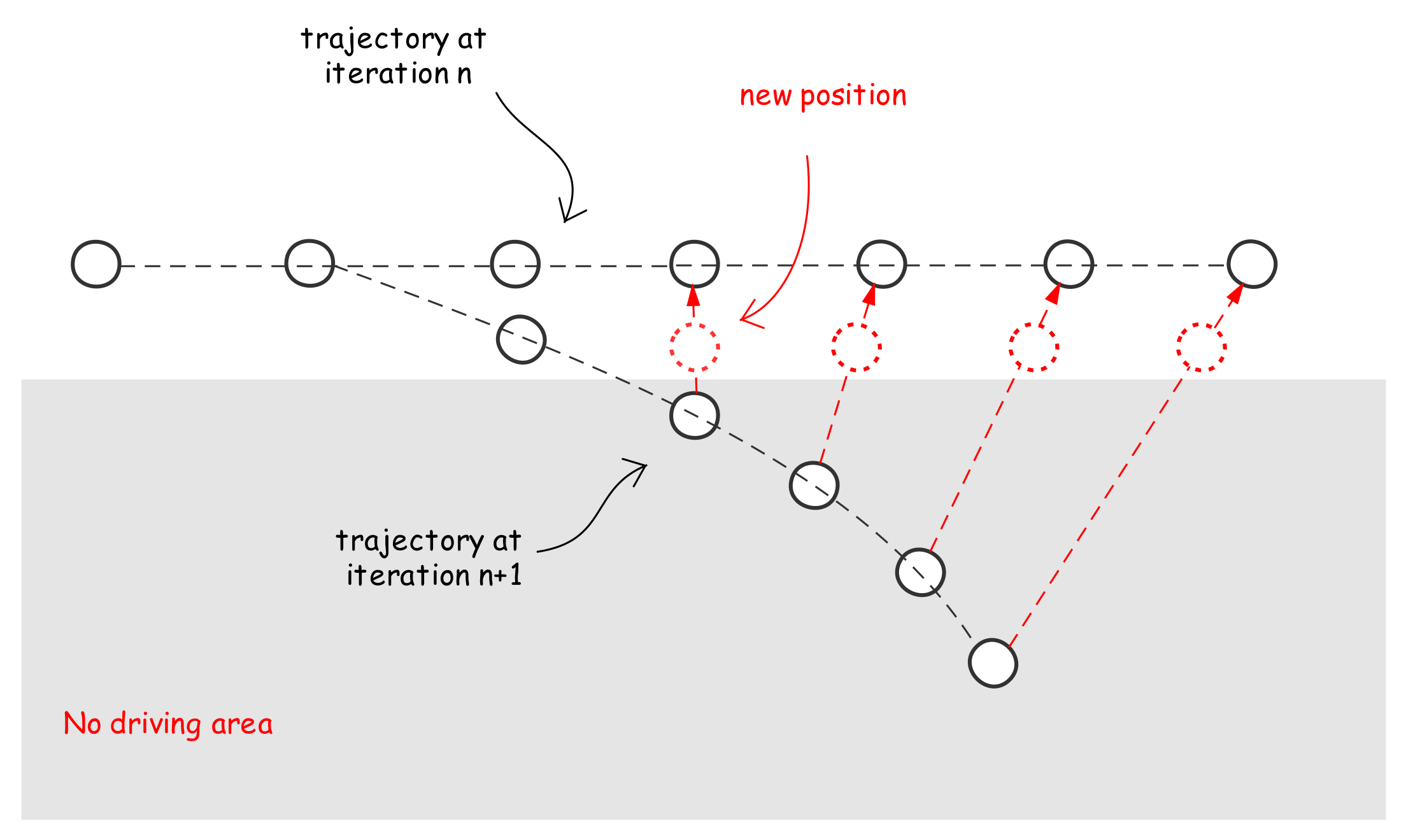
    The final trajectory is a linear combination of the solution at different iterations, and is therefore guaranteed to be within the (static) boundaries of the road.
  • The new framework was implemented and validated using Matlab and Pro-SiVIC simulations in different emergency scenarios, using both algorithms. The corresponding performance results are evaluated.

1.4. Organization

The structure of this paper follows these three contributions. Section 2 presents first the decision-support previously developed at Eiffel University, then the expanded framework and its components. Section 3 presents the emergency trajectory planning algorithm and its implementation. Section 4 shows the simulation results of our two trajectory planning algorithms in different near-accident scenarios, while Section 5 analyzes the results in details and discusses future research directions.

2. Autonomous Decision Support Framework

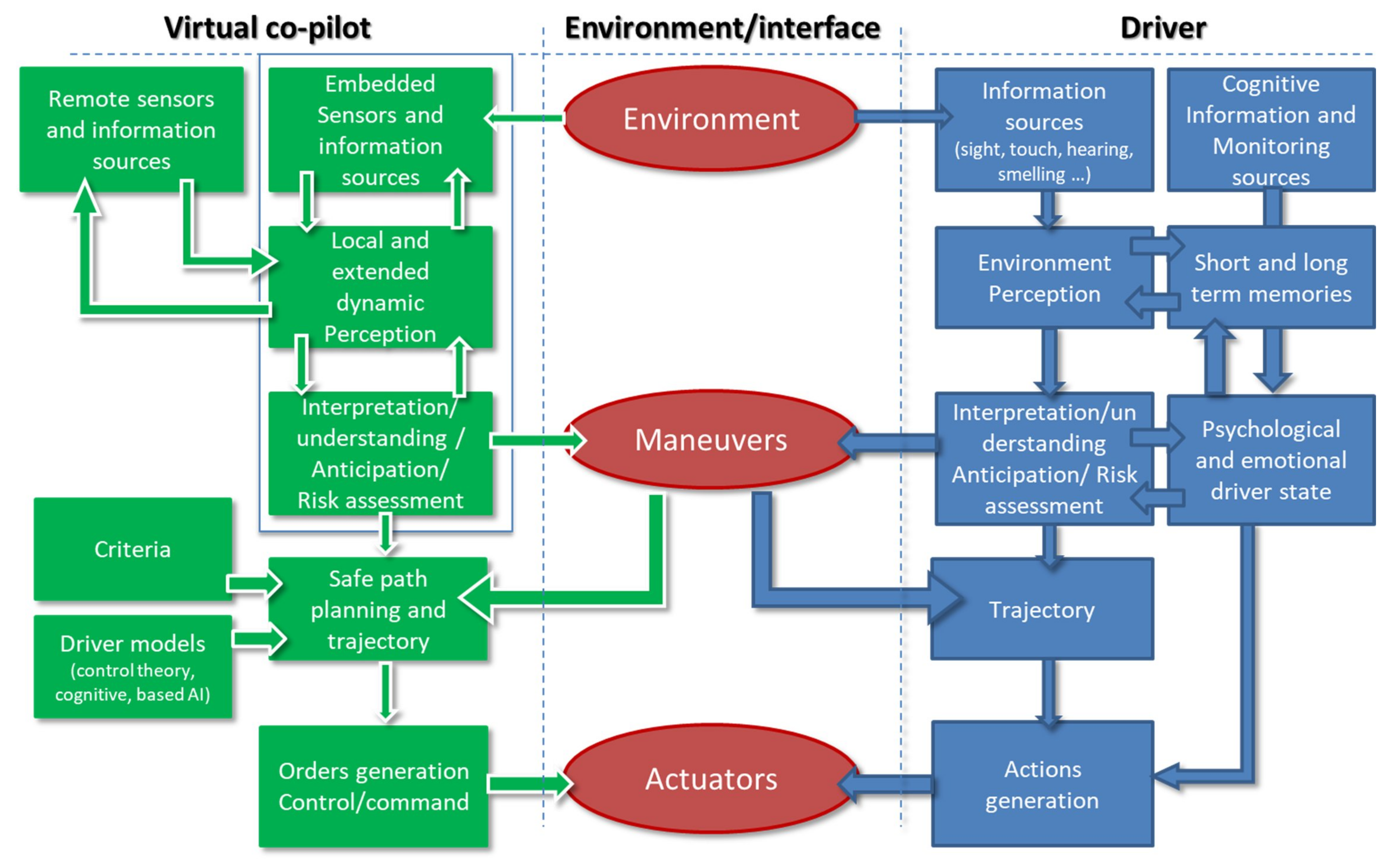
2.1. Autonomous Driving and Virtual Co-Pilot

The Decision-support framework presented in this paper is based on the concept of “virtual Co-Pilot” developed over the past few years at Gustave Eiffel University (see Appendix A). As part of a European project (HAVEit [64]) and a French project (ABV [66]), some components needed for the design of a virtual Co-Pilot framework involving the perception, decision, path planning, and control modules have been developed at Gustave Eiffel University [64] as a highly automated driving delegation application shared with a human driver for Highway situations. This optimal path planning application (minimization of a set of criteria including risk) tackled a multi-constrained problem. In terms of general architecture, the functions developed for the virtual Co-Pilot are very similar to human operations and behaviours (see Figure 2).
The virtual Co-Pilot can guarantee a high level of legal safety regarding the road environment. To do that, the Co-Pilot uses human and traffic rules to guarantee safety and efficiency in mixed traffic (with other non-equipped vehicles and users).
Its application domain is defined as an operating space guaranteeing the safety of users when all road users respect the traffic rules. In this Operating Driving Domain (ODD), all the necessary strategies are implemented to avoid collisions or, in the worst-case scenario, to mitigate them, using emergency strategies. In autonomous mode, the Co-Pilot considers several constraints, such as the target speed and the target lane of traffic.
Finally, the human can be put in the loop, using specific mechanisms to allow the human driver to share the driving task with the virtual Co-Pilot. A few years ago, this active and/or informative human/machine interaction was a great challenge. The sharing of the driving task simultaneously by the ADS and the human driver will not be addressed in this paper but can be found in [64].
Some of the key ideas and algorithms of the virtual Co-Pilot are presented in Appendix A. The next section will present an expanded decision-support framework, built on this Co-Pilot.

2.2. New Framework Design

One of the limitations of the Co-Pilot presented above is its assumption that all road users follow its set of human and traffic rules. As a result, it is possible to reach an emergency situation where the Co-Pilot cannot find a collision-free trajectory in specific extreme scenarios (examples of these are shown in Section 4.2.3).
As part of the European Trustonomy project [65], the Co-Pilot was integrated into a more general Automated Decision-Support Framework (ADSF) to avoid these emergency situations if possible and propose a safe answer otherwise. The main innovation in this framework, which is illustrated in Figure 3, is its use of two independent trajectory planning algorithms (the “autonomous” and “emergency” algorithms), together with a specific module to switch between modes depending on the situation. The autonomous mode uses the planning algorithm developed for the Co-Pilot, while the emergency mode uses a new and specific algorithm for emergency situations, detailed in Section 3. The early warning module was added to try to prevent emergency situations whenever possible, especially in “human driving” mode (when the Co-Pilot is not used), and is detailed in [68]. In the Trustonomy project, the Decision-support module also interacts with the HMI (Human-Machine Interface) and DIPA (Driver Intervention Performance Assessment) modules, but these interactions are not detailed in this paper.

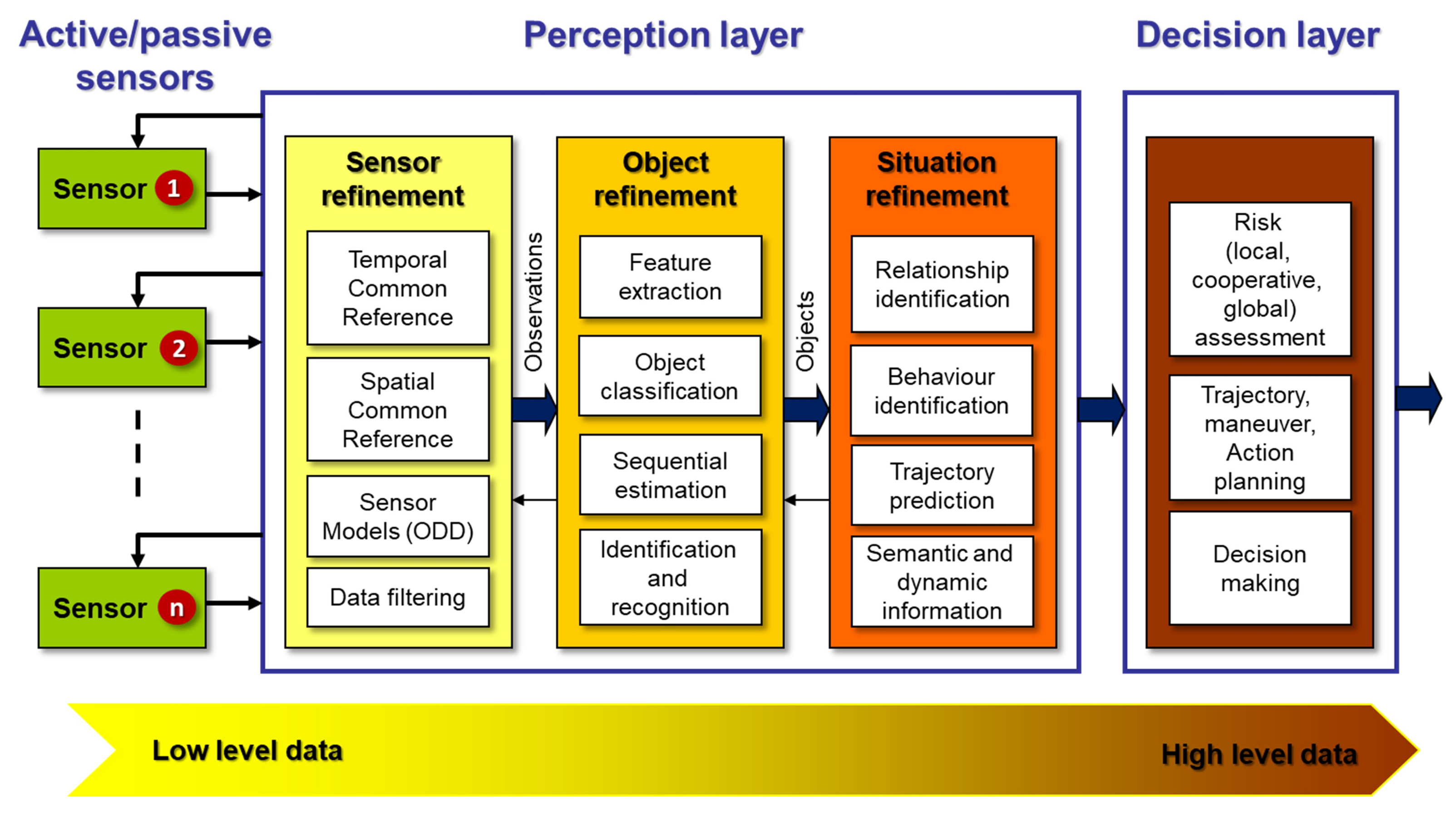
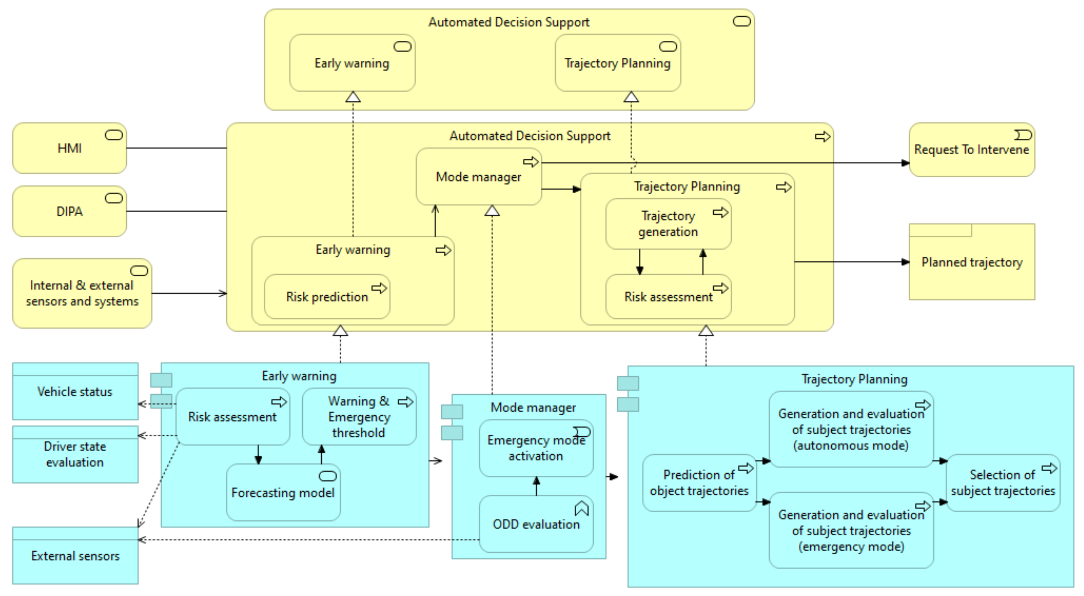
2.3. Component Overview

As shown in Figure 3, this framework is divided into three major components:
Early warning:
The role of this component is to monitor and forecast different risk levels and indicators. Those risks are relative to the main road key components (obstacles, road attributes, ego-vehicle, environment, driver). Each calculated risk depends not only on the current state of the component itself but also on a forecast of its evolution. Thus, each risk has two thresholds (warning and emergency) and three driving states (regular, cautious/degraded, and emergency/critical). When a risk is higher than the warning threshold, the associated warning is sent to the driver via the HMI, whereas the emergency threshold is used directly by the Mode manager. This component is presented in details in [68].
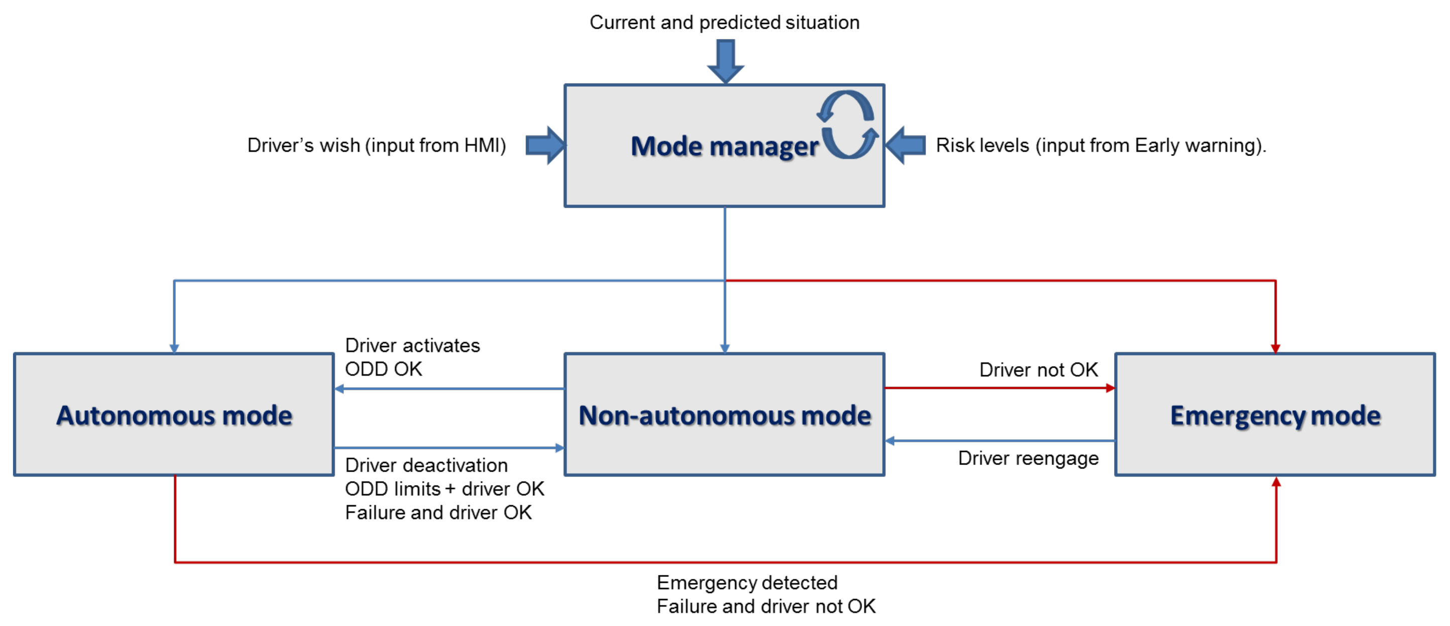
Mode manager:
This component decides which driving mode should be adopted, depending on the current and short time predicted situations, the driver’s wish (input from HMI), and the combination of the different risk levels (input from Early warning). The ODD establishes conditions under which the vehicle may operate in autonomous mode. The Mode manager is also responsible for starting the emergency mode and issuing a request to intervene to the human driver.
Trajectory planning:
This module generates the trajectories, which the vehicle tracks in autonomous and emergency modes. It uses inputs from the perception module to predict the trajectories of the different objects/obstacles in its environment. It then generates, evaluates and selects the best trajectory for the ego-vehicle. This trajectory must respect a set of constraints (traffic, system, driver rules) relative to safety. Depending on the mode, it uses either the classical Co-Pilot algorithm (see Appendix A) or the new emergency algorithm (see Section 3).

2.4. Mode Transitions

The ADSF can send warnings to the driver (in non-autonomous mode), request to intervene (in autonomous mode) or start the emergency mode (at any time). In non-autonomous mode, the human driver controls the vehicle, the trajectory planning module is turned off, and the Early Warning is monitoring the driving risks. In autonomous mode, the ADSF controls the car, and the three components are active simultaneously. In emergency mode, the early warning component is turned off, and the trajectory planning component takes inputs from the vehicle status and environment perception data. The transitions between those different modes are operated as shown in Figure 4.

3. Emergency Trajectory Planning Algorithm

In order to build an efficient emergency trajectory allowing to take into account the level of criticality of the current situation, the emergency function of the automated decision support is made of two blocks. One is the emergency trajectory planning which rapidly produces candidates for emergency trajectories and the other one is an “ethical” based decision module. According to an IEEE study on ethics [69]: “Society has not established universal standards or guidelines for embedding human norms and values into Autonomous and Intelligent Systems today. However, as these systems are instilled with increasing autonomy in making decisions and manipulating their environment, it is essential they be designed to adapt, learn, and follow the norms and values of the community they serve.” Thus, the idea of Trustonomy project is to implement human norms and test them, as a first stone on the way of ethically designed autonomous decision systems.

3.1. New Emergency Mode

Although the model used in the virtual Co-Pilot (referred to as “the Vanholme’s model” thereafter [64]) is able to provide efficient strategies for different autonomous driving scenarios and different autopilot styles, its decision-making abilities are limited in certain specific situations:
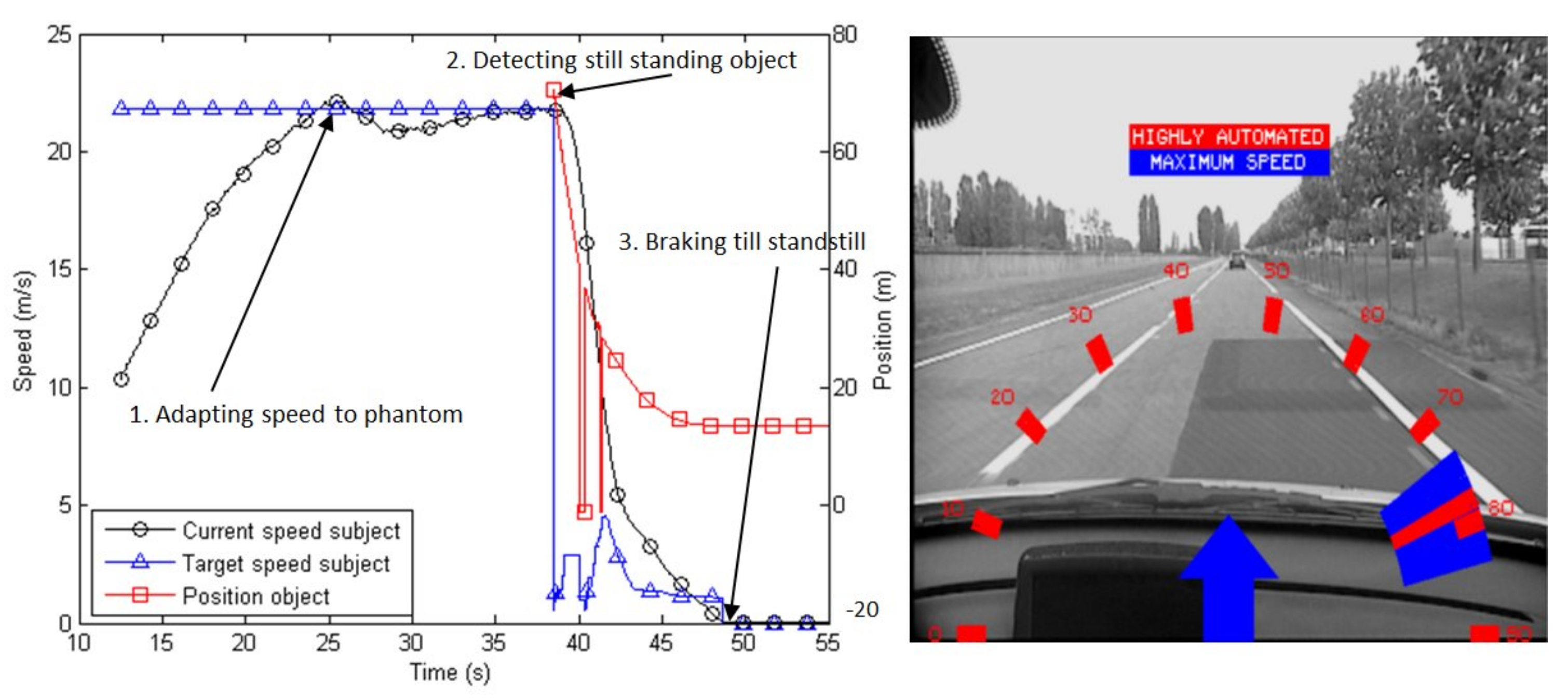
  • In this model, the only option proposed in case of emergencies (no collision-free solution found) is an emergency braking to mitigate the collision. Although this answer can work in certain low-speed driving situations, we cannot expect the vehicle to have sufficient braking distance to avoid a collision when entering emergency mode even at medium speed. Meanwhile, a different decision, such as steering rapidly to avoid an obstacle instead of braking, may allow to avoid collisions altogether. It follows that this single option (safe braking) makes the Vanholme’s model less adaptable in emergency situations.
  • The Vanholme’s model was designed to react to emergency situations while driving in autonomous mode. The ego vehicle takes the corresponding actions based on certain rules, and all the decisions are made in a fully autonomous driving environment. However, when the emergency mode is force switched from manual mode because of unsafe behavior or visual constraints of the driver (e.g., following with high speed and close distance, invisible obstacles), preconditions in emergency mode will be uncertain for the vehicle and namely lead to Vanholme’s model going to an unknown state, then fails in reducing the risk of collision.
In our new decision-support framework, a new trajectory planning algorithm was proposed specifically for these emergency situations, when the Vanholme’s model cannot find a collision-free trajectory. This new algorithm is based on Elastic Bands theory. Having as inputs the road environment and the obstacles state together with the normally planned trajectory (from the previous section), the emergency planner adapts the initially planned trajectory to avoid any collision with the detected obstacles while keeping the vehicle on a safe road. This module then outputs potential candidates to be activated in a decision module. The basic principle of this relies on the EBs which seek minimal deformation of the original trajectory. This algorithm has been improved in 2003 by the team of Hilgert et al. [51]. The module proposed in this ADS is mainly based on the works from Brandt et al. in 2005 [70] (see Figure 5). Our new algorithm in this paper combines an improved internal force based on the classic EB method and external force provided by the common artificial potential method. When the vehicle goes into emergency mode, the trajectory can be computed based on the physically acting of these two types of forces, which results in the mode being able to provide multiple solutions based on the different obstacles and road information. In addition, the previous state(speed and orientation) of the vehicle will be also considered in the computation of internal forces in order to simulate a more realistic dynamic process of collision avoidance. Based on these improvements, whether the emergency mode is switched from autonomous mode or manual mode, the model can quickly generate an optimal trajectory with mechanical feasibility to react to current situations.
Thus, it can be seen that the decision-making model combing Vanholme’s model for autonomous mode and the new improved trajectory planning for emergency mode is able to provide more efficient and feasible solutions based on the different scenarios of autonomous driving (even combining with manual driving), especially for some uncertain emergency situations.

3.2. Internal Force

The general Elastic Bands method simulates a trajectory through a series of nodes r t representing the positions of the vehicle, at different times t in the immediate future. Usually, each pair of consecutive trajectory nodes is linked by a spring so that they stay at a relatively constant distance from each other (see Figure 5). The total contraction force F t c o n t applied to node t is computed as shown in Equations (1) and (2):
F t c o n t = F t Δ t , t c o n t + F t , t + Δ t c o n t
F t , t + Δ t c o n t = k c o n t r a c t i o n · ( | | r t + Δ t r t | | l 0 ) · r t + Δ t r t | | r t + Δ t r t | |
where F t Δ t , t c o n t (resp. F t , t + Δ t c o n t ) is the contraction force from the previous (resp. next) trajectory point. The spring original length l 0 and coefficient k c o n t r a c t i o n are free parameters. Since the internal force of the trajectory node is only calculated based on the neighbouring nodes in the classic algorithm, the state of the previous time step does not have any influence on the current time step, which is not able to satisfy a continuous and dynamic process in the trajectory planning. Considering this limitation of the classic algorithm, we redefine the internal force as shown in Equation (3):
F t i n t e r n a l = k i n t e r n a l · ( r t E q u i l i b r i u m r t )
where F t i n t e r n a l is the internal force on the current trajectory point, r t is the node position of current time step. and the coefficient k i n t e r n a l is free parameter. r t E q u i l i b r i u m is the equilibrium position of current node, which is computed based on the positions of previous two nodes and next nodes. When these three points are collinear, the equilibrium position can be simply calculated as r t Δ t + ( r t + Δ t r t 2 · Δ t ) 3 . On the contrary, current equilibrium position is calculated based on the arc established by previous two nodes and next nodes, which satisfies that θ 3 θ 2 = θ 2 θ 1 (see Figure 6).
In classical EB, the first trajectory node (current position) and the last one (target) are fixed in advance, then forces apply to the nodes in the middle. Therefore, the result is largely related to the position of the last point on the band, which may cause the trajectory of the current situation is not optimal. For example, when the fixed last point is near to the obstacle, the vehicle may lose an early deceleration opportunity, namely the risk of collision has been increased. Besides, the attraction of the last node may lead to some mechanically unrealistic trajectories, when the vehicle is pushed by strong external forces. This problem is manifested in the sudden changes in the speed and direction of the last few trajectory points. Based on these problems, our approach defined a movable last point depending on the previous two trajectory nodes (see Equation (4)), accordingly provided a more optimized solution in some emergency situations.
F t l a s t i n t e r n a l = k i n t e r n a l · ( 2 · r t Δ t r t 2 · Δ t r t )
where F t l a s t i n t e r n a l is the internal force on the last trajectory point, which is different to the fixed last trajectory point of the classical EB method.
As mentioned in the last section, compared to the classical EB method, the new internal force also considered the state of the previous two nodes. The reasons are due to the potential problems specifically linked to emergency situations, which are often ignored in the literature. The first problem related to emergency situations is that if the obstacle is very close, a simple contraction/repulsion algorithm might end up contracting all the nodes towards the current position of the car, ignoring the current speed of the car (see in Figure 7), which is lack of mechanical feasibility. In the above emergency situations, the classic method also ignored the previous orientation of the car, which is the second problem (see in Figure 8). To avoid these abrupt changes in the vehicle orientation and velocity, especially between the first and second nodes, the internal force is applied to each node depending on the relative orientation and distance of the previous two nodes and the next node, which ensures that steering and speed changes of the vehicle are in a gradual process (see in Figure 7 and Figure 8).

3.3. External Force

As is common in the literature, the potential of the road prevents the vehicle from leaving the boundary and keeping its current lane on the road. When the vehicle drives out of the boundary, the value of the potential U b o u n d a r y t ( x ) should become infinite. In the meantime, the potential will also give a relatively weak potential U l a n e t ( x ) to the vehicle when it drives on a certain lane (as in Figure 9). Thus, a repulsive force is employed according to Equation (5):
F e x t e r n a l , r o a d t = [ U b o u n d a r y t ( x ) + U l a n e t ( x ) ] = u r o a d · ( k l a n e · ( x s i g n ( x ) · w 2 ) + k b o u n d a r y · ( 1 p + x 1 p x ) )
where F e x t e r n a l , r o a d t is the external force provided by the road potential. u r o a d is the direction vector (left side to the right side) of the x-axis in the relative coordinate system, and x is the current position in this coordinate system. The boundary force acting on the vehicle is in the area p w , where w is the width of the lane, the length of p is slightly bigger than w. Coefficient k l a n e and k b o u n d a r y are free parameters.
The external force also aims to keep the current vehicle a safe distance d0 away from other dynamic or static obstacles by building an obstacle potential U o b s t a c l e t ( x ) that rises to infinite strength when any other vehicles approach any part of them. In some emergency situations, steering to avoid is encouraged instead of stop, which means a shaped obstacle potential is desired. Thus, we choose an obstacle force as shown in Equation (6):
F e x t e r n a l , o b s t = [ U o b s t a c l e t ( x ) ] = u o b s · k o b s · ( 1 d 1 d 0 ) · ( 1 d 3 )
where F e x t e r n a l , o b s t is the external force provided by the obstacle potential, u o b s is the direction vector from the center of the obstacle to the current point. d is the distance to the boundary of the obstacle, and k o b s is a positive constant. In order to take into account moving obstacles, each node at time step t has its own environment and therefore its own potentials U t , and the external force acting on this trajectory node is the sum of the forces provided by these potentials.

3.4. Dynamic Process

This proposed algorithm starts with an initial collision-free exploring trajectory of n nodes, representing the position of the vehicle at different times in the future. The total force F t o t a l ( i ) applied to a node at iteration i is given in:
F t o t a l ( i ) = F i n t e r n a l ( i ) + F e x t e r n a l ( i )
where F i n t e r n a l ( i ) , F e x t e r n a l ( i ) represent respectively the internal force, external force on the current node at iteration i. During the planning step, the trajectory nodes move under the action of total force applied to them for several iterations, until an equilibrium state is reached where the total force on each node is approaching zero. This step must be fast enough to ensure real-time operations. For this reason, second-order computation is employed to compute displacements between trajectory points at each iteration as in Equation (8), which can provide a fast convergence compared to directly applying the forces on the trajectory nodes.
q ( i + 1 ) = M t o t a l ( i ) F t o t a l ( i ) + q ( i )
where q ( i + 1 ) is the positions of trajectory at iteration i + 1 . M t o t a l ( i ) represents the total matrix derivative ( 2 n * 2 n Hessian matrix) of the total applied forces, namely the sum of the matrix derivative of each force at iteration i. F t o t a l ( i ) is the forces acting on the trajectory at iteration i, and q ( i ) is the positions of trajectory at iteration i (see Equation (9))
F t o t a l ( i ) = [ F t o t a l 1 ( i ) , F t o t a l 2 ( i ) , . . . , F t o t a l n ( i ) ] q ( i ) = [ r 1 ( i ) , r 2 ( i ) , . . . , r n ( i ) ] M t o t a l ( j , k ) ( i ) = d F t o t a l ( j ) ( i ) d q ( k ) ( i )
One problem occurs when second-order computation is employed, the trajectory node may go into the non-driving area (inside the obstacle, out of boundary) due to a large displacement. In order to solve this problem, we added a new computation (see Equation (10)) at each iteration in this area, as shown in the Figure 10. When the trajectory node is detected at the non-driving area at iterations i + 1 , the possible biggest k is chosen to ensure that the new position is in the driving area, and it is determined k with the value of 0 can still work in the worst case. In addition, k is 1 for the nodes that are already in the driving area.
q n e w ( i + 1 ) = k · q ( i + 1 ) + ( 1 k ) · q ( i )
where q n e w ( i + 1 ) is the new positions of trajectory in driving area at iterations i + 1 . k is a array of positive coefficients in the range of 0 to 1.
The final trajectory is then selected and sent to the vehicle controller. At the next iteration, the exploring trajectory starts at the new position of the vehicle, and uses the last n 1 points of the final trajectory; one last point is added assuming constant speed and steering. The environment data is updated (obstacle positions and speeds, road, etc). The emergency algorithm stops when the vehicle has stopped (or crashed), or if either the driver or the autonomous mode is ready to take over.

4. Results

4.1. Results in Normal Driving Conditions

In order to test, evaluate and validate the performance and capacities of this Co-Pilot, a set of use cases have been implemented in both real and virtual environments. The purpose is to confirm that the Co-Pilot is able to guarantee reliable, robust and, above all, safe operating and driving behavior in relation to different rule categories. The different scenarios used and tested were “approaching a speed limit”, “approaching a vehicle or a ghost zone”, “following a target”, and “overtaking a vehicle”.
It is important to note that this virtual Co-Pilot (ADS) was prototyped and developed using the Pro-SiVIC platform (ESI group), coupled with the RTMaps platform (Intempora). Pro-SiVIC (presented in Figure 11) is a 3D simulation software designed for autonomous vehicle prototyping, test, evaluation, and validation: it features complex environments, realistic modelling of the vehicles, and of all the embedded sensors (cameras, radars, lidars). RTMaps is a data processing platform that controls the car and does all the trajectory computations, either in simulation (when connected to Pro-SiVIC) or in the field (when implemented on a real vehicle).
In order to be able to concentrate solely on the development of the virtual Co-Pilot, the perception section was generated by the Pro-SiVIC “observers”. These “observers” were “ground truths” sensors that provided data and by extension, perfect perception. In order to validate the reliability and robustness of the suggested method, we ran scenarios with 5 and 10 vehicles, each with its own Co-Pilot configured for one of the three driving modes (“comfortable”, “normal”, “sporting”). On the HMI presented in Figure 11, we can observe the use of an instruction matrix for possible maneuvers and reachable zones (size 3 × 3). The first cell represents a left lane change and acceleration. The second cell represents a simple acceleration. The fifth cell represents a constant state (constant position and speed). The 9th cell represents a right lane change and deceleration. As we can see, the cells in red represent impossible maneuvers (trajectories, speed profiles) after the evaluation stage.
Once the results obtained in the simulation were considered to be of sufficiently good quality, the Co-Pilot application was embedded into one of Eiffel University’s prototype vehicles dedicated to automated driving systems (presented in Figure 12) [64]. For these real tests on test tracks, the dynamic local perception map was built from a set of modules and functions allowing assessing the state of all relevant road key components (obstacles, road, ego-vehicle). The obstacle detection and tracking were made with a cooperative fusion approach. This cooperative fusion approach used either a dense stereo vision system and a lidar [71], or a mono camera system and a lidar [72]. For the dynamic assessment of the road objects, a robust and efficient tracking stage based on the belief theory has been applied in [73]. For the road markings and lanes detection and tracking, the work developed in [74,75] was integrated in the perception architecture. This road-centered part allowed managing multiple lane configurations and lane changes without discontinuities and interruptions. About the localization and ego-vehicle state assessment, an Interacting Multiple Model (IMM) approach adapted for unusual vehicle state and maneuver has been proposed [76]. The fusion of data coming from lateral cameras, HD Maps, and the IMM approach provides a very accurate lateral positioning [77]. It is essential for lane changing and overtaking maneuvers. This full perception architecture is presented in Figure 12.
Figure 13, Figure 14, Figure 15 and Figure 16 present the results obtained for the first three use cases with the embedded Co-Pilot in a real prototype, used on the Versailles Satory’s test tracks. In Figure 13, we can clearly see the adaptation of the vehicle speed to a constraint (new speed limit). Figure 14 shows the reaction of the Co-Pilot recognizing a “ghost” vehicle after having detected an obstacle. Figure 15 shows a target tracking scenario, with the target making gear changes and one lane change. Finally, Figure 16 shows an overtaking scenario involving both longitudinal and lateral maneuvers.

4.2. Results in Emergency Driving Mode

The previous section presented four simulations in different scenarios, for which the Co-Pilot was initially designed and can handle easily. However, when put in more difficult situations, like the two presented in Section 4.2.3, the Co-Pilot alone could not find a safe trajectory and collided with the obstacle. The simulations presented below will showcase the abilities of our new framework and of the emergency algorithm used in combination with the Co-Pilot.

4.2.1. Parameters Values

In Table 1, the adopted parameters are enumerated for the simulations in Matlab and Pro-SiVIC. In this paper, we use the same parameters both in Matlab and Pro-SiVIC, in order to make a comparison and validation of the simulation results. It is worth mentioning that the strength of the internal force is fixed to constant 1, other problem parameters are tested based on this value and other indices. In addition, the state variables k is an array with all ones initially since the initial exploring trajectory is collision-free. Once some nodes of the new exploring trajectory locate in the non-driving area, the corresponding element in k will change according to the current and the previous position of the node to ensure that the trajectory nodes are always in the driving area.

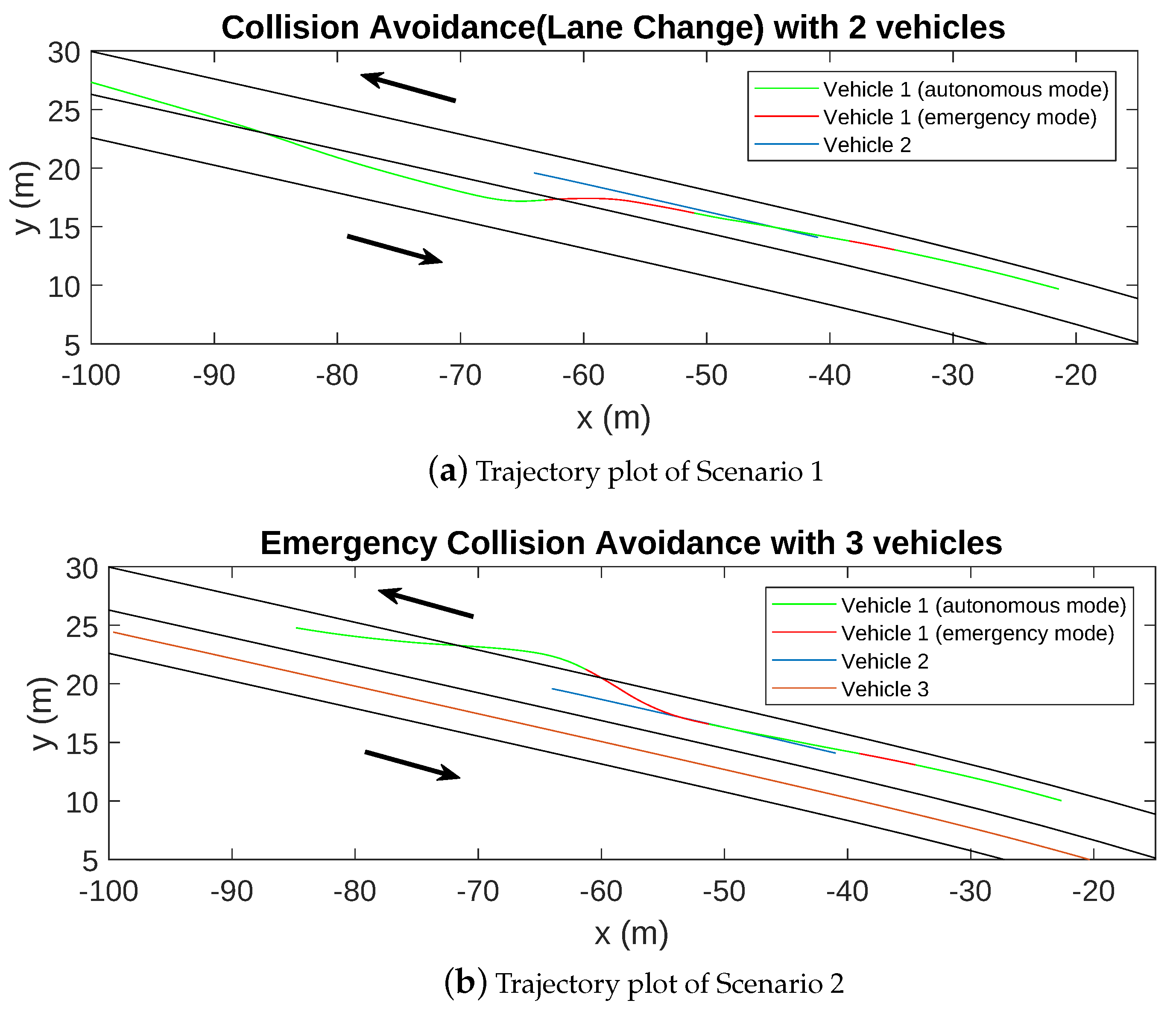
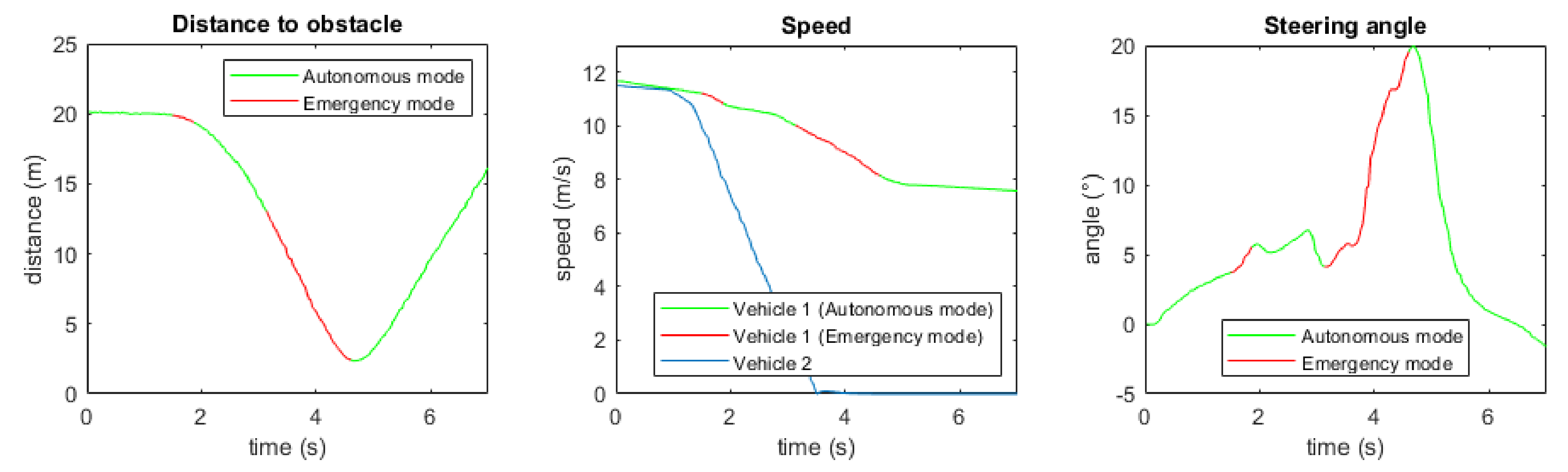
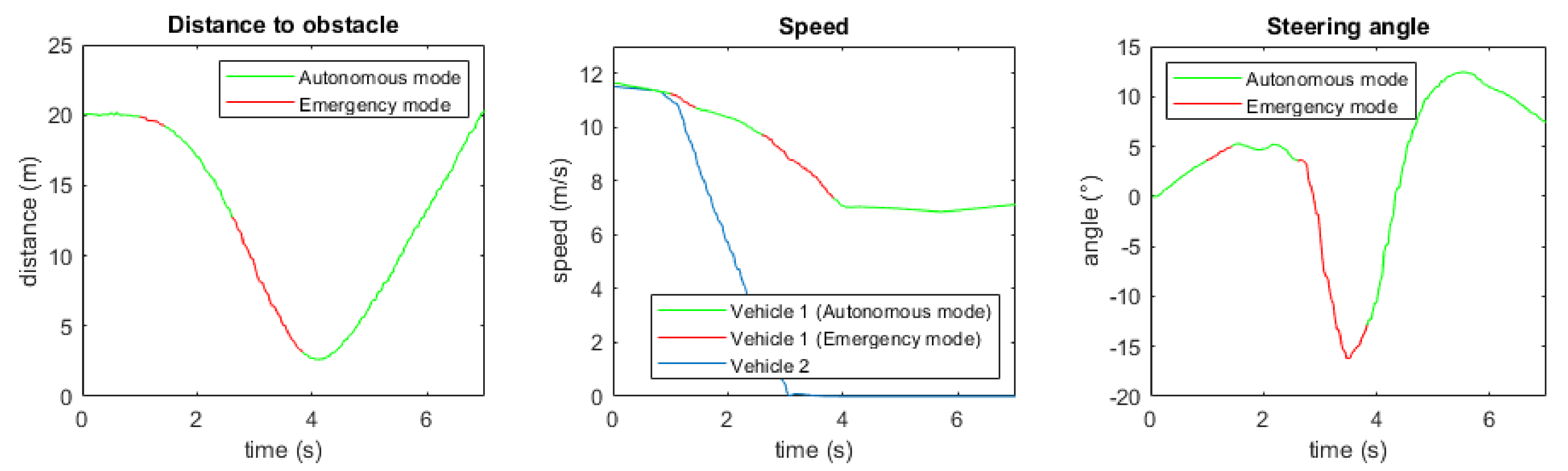
4.2.2. Simulation in Matlab

The Emergency Trajectory Planning Algorithm was first implemented and validated in Matlab, in order to calibrate the different parameters of the model. For these preliminary tests only the emergency algorithm was used, and not the full framework. The results are presented below.
In these simulations, the ego vehicle was crossing an intersection from south to north and has priority (e.g., green light), while another vehicle crossed from east to west without stopping or slowing down. The simulation started when the other vehicle was detected and the ego vehicle switched to emergency mode to quickly adapt its trajectory and avoid the collision if possible. Figure 17 shows the external potential corresponding to both the roadside and the other moving vehicle.
In the first scenario (Figure 18a), the ego vehicle was able to avoid the collision by accelerating and steering slightly to the left, in order to cross the intersection in front of the other vehicle. After the intersection was passed, it went back to the middle of the road and to its normal speed. In the second scenario (Figure 18b), the ego vehicle slowed down and let the other vehicle pass first to avoid the collision. In the third scenario (Figure 18c, the ego vehicle met a long, slow-moving vehicle (such as a truck) at the intersection. In this situation, it had to brake hard, almost coming to a complete stop, before passing the intersection right behind the other vehicle. Finally, in the fourth scenario (Figure 18d), the intersection was completely blocked and the ego vehicle had to do an emergency stop.

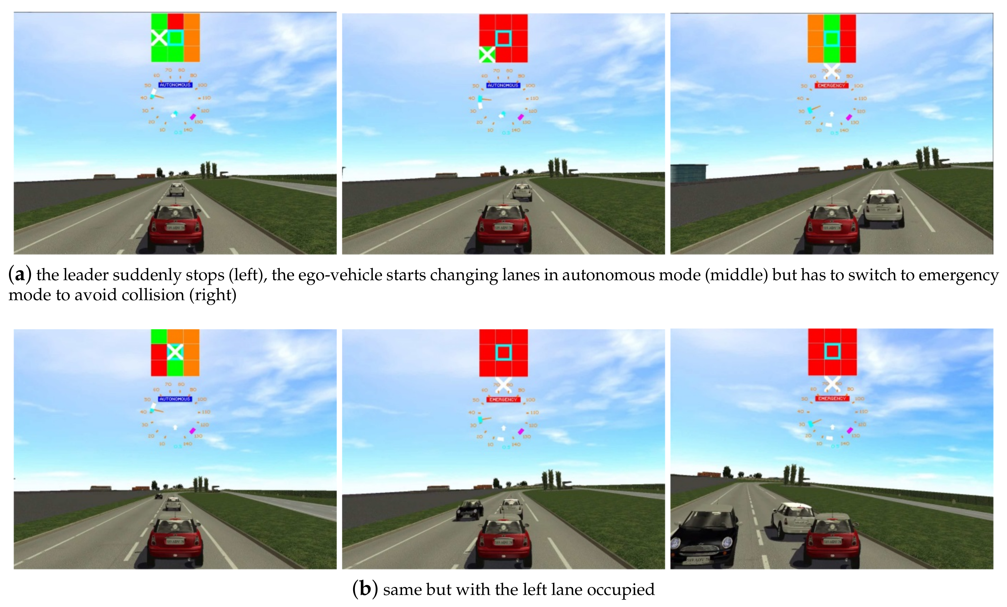
4.2.3. Simulation in Pro-SiVIC

The next phase of testing the Automated Decision-Support Framework was again in the simulation, this time using two interconnected softwares Pro-SiVIC and RTMaps (Intempora).
In the two scenarios presented here, the ego-vehicle (the red car on Figure 19) started in Autonomous mode (using the virtual Co-Pilot presented in Section 3), relatively close to another vehicle (the white car), which did an emergency braking at 1 second, coming to a complete stop about 2 s later. The ego vehicle switched to Emergency mode (using the emergency trajectory planning algorithm presented in Section 4) and tried to avoid the collision. These scenarios were designed to show the limits of the Co-Pilot, and demonstrate how the emergency mode could help in these critical situations.
Figure 20a,b show the trajectory plot for all cars in both scenarios. In the first one (Figure 20a), the left lane was available. Autonomous mode was engaged and the advice was given to change lane and keep the same speed in order to overtake the white vehicle. Unfortunately, the white vehicle applied emergency braking. The only way for the virtual Co-Pilot to avoid the collision was to change lanes and apply a braking maneuver. The two vehicles were too close and a collision seemed to be unavoidable. The emergency mode was activated and an abrupt steering wheel order was given in order to avoid the collision. In the advice matrix, the right column was fully inaccessible. Now only the left lane was green. In the second one (Figure 20b), the autonomous mode was engaged. The advice was given to stay in the same lane at the same speed. The left lane was unavailable due to the presence of a third vehicle (the black vehicle) moving in the opposite way. Unfortunately, the white vehicle applied emergency braking. The red vehicle tried to overtake the white vehicle but could not apply this maneuver due to the black vehicle. The only way was to switch to the emergency mode. The emergency mode advice was to use the emergency lane (or sidewalk) in order to avoid collision with both the black and the white vehicles.
Figure 21 and Figure 22 show the distance between the two cars, the speed of the vehicles 1 and 2, and the steering angle of the ego-vehicle, as a function of time during the simulation, for both scenarios. In all plots (as well as the trajectory plots above), the ego-vehicle mode is indicated by the color: green for Autonomous mode (Co-Pilot), and red for Emergency mode. The first scenario shows the limits of the lateral maneuvers of the Co-Pilot: the steering angle stayed cautious and rarely exceeded 7 degrees in Autonomous mode (see Figure 21), which was not enough given the urgency. In Emergency mode, the steering angle reached up to 20 degrees. Lane changing was normally a maneuver that the Co-Pilot was capable of doing, but not in such a short time interval. As soon as the obstacle was safely passed, the ego-vehicle switched back to Autonomous mode and converged toward a cautious and soft driving behavior. The second scenario aims to demonstrate the emergency algorithm’s flexibility, its ability to ignore traffic rules and laws and come up with creative options that the general Co-Pilot would never consider. Since the two legal lanes were occupied, the Co-Pilot simply could not find a trajectory with no collisions. However, the Emergency mode was able to use the space between the white car and the sidewalk.
In an emergency situation like that, the ability to ignore the lane structure and only focus on the position of the obstacles was an advantage compared to the traditional lane choice and speed profile selection used in the Co-Pilot.
In both of these scenarios, slightly different initial conditions (speed, initial distance, deceleration of the leader vehicle) were tried in order to verify the algorithm’s robustness.

5. Discussion and Conclusions

This paper introduced the Autonomous Decision-Support Framework, developed by Eiffel University for the EU project Trustonomy, and focused on the problem of trajectory planning in emergency situations. Some results of the virtual Co-Pilot were given in a simulation environment (Pro-SiVIC and RTMaps) and embedded in a real prototype. A complementary algorithm specifically designed for emergencies has been proposed and developed in order to propose unusual maneuvers allowing taking into account critical situations. At this moment, this “emergency” system has been developed and tested in simulations, using Matlab and Pro-SiVIC. Its main characteristics are the following.
  • It is based on EB’s trajectory generation, for fast computation.
  • Unlike in classical methods, the last point of the trajectory is not fixed, but simply attracted to the general direction of motion, to give more flexibility in different emergency situations.
  • The current orientation and speed of the vehicle are taken into account using additional ad hoc forces during the trajectory generation, to ensure mechanical feasibility even when obstacles are very close.
This algorithm was used in the Trustonomy framework for risk management, where the decision-support module can switch between the normal Autonomous mode and this new Emergency mode depending on the risk level. Simulation results in a realistic 3D environment showcased the benefits of this hybrid approach in near-accident situations.
However, the simulations presented here have several limitations which will have to be tackled in future works. First, this model has many free parameters, so the calibration step to balance the different forces requires a special attention, to ensure the highest level of safety in any situation. The behavior of the vehicle when the collision is unavoidable (or when the trajectory given returned the algorithm is not feasible) is not clearly defined at the moment. The prediction of the movement of obstacles in dynamic settings is very basic at the moment and could be improved. Finally, interactions and driving sharing with the human driver of the ego-vehicle was not taken into account in the emergency part, although it has been used with Vanholme’s model before, this paper was only concerned with how the vehicle would react in an emergency situation, and not the pair vehicle and driver.
As the Trustonomy project continues in 2021, the next steps of developing an autonomous Decision-Support framework are the following.
  • Calibration and testing of the Emergency trajectory planning algorithm will be continued in different scenarios (urban, scenarios with multiple vehicles, pedestrians, etc).
  • The current algorithms will be included in the general ADSF framework, which includes a Driver State Monitoring system and a Driver Intervention Performance Assessment (DIPA) module to monitor mode transitions and driver-related risk management at all times.
  • The general framework will be tested on a new real vehicle in 2021 in France, possibly using virtual obstacles generated from Pro-SiVIC platform (Vehicle in the Loop architecture with communication means).
  • Different perception architectures and perception data will be used in order to assess the capability of the full ADS in adverse and degraded conditions involving possible sensor failures.

Author Contributions

Conceptualization, O.O. and D.G.; methodology, O.O.; software, W.X.; validation, W.X. and R.S.; formal analysis, R.S.; writing—original draft preparation, W.X.; writing—review and editing, D.G.; visualization, W.X.; supervision, D.G. and R.S.; project administration, O.O. All authors have read and agreed to the published version of the manuscript.

Funding

This paper is supported by European Union’s Horizon 2020 research and innovation program under grant agreement No. 815003, project Trustonomy (Building Acceptance and Trust in Autonomous Mobility).

Data Availability Statement

Data sharing not applicable.

Acknowledgments

The authors wish to thank Benoit LUSETTI for his contribution in validation.

Conflicts of Interest

The authors declare no conflict of interest.

Abbreviations

The following abbreviations are used in this manuscript:
ADSAutonomous Driving System
ADSFAutonomous Decision Support Framework
AIArtificial Intelligence
APFArtificial Potential Field
AVAutomated Vehicles
Co-PilotCooperative Pilot
DIPADriver Intervention Performance Assessment
DSMDriver Status Monitor
EBElastic Band
ESIEngineering System International
HMIHuman-Machine Interface
IEEEInstitute of Electrical and Electronics Engineers
IMMInteracting Multiple Model
ODDOperational Design Domain
Pro-SiVICVehicle, Infrastructure and Sensors Simulation Platform (French acronym)
RRTRapidly-Exploring Random Tree
RTMapsReal-Time Multisensor Applications
SAESociety of Automotive Engineers

Appendix A. Cooperative Pilot

This section presents some of the components of the virtual Co-Pilot developed at Eiffel University over the years [64,66], that were directly integrated into the new Decision-Support framework.
In order to design and develop the ADS module and offer to the control module at least one admissible trajectory, four steps are necessary. The first one consists of bringing the data from the perception layer by estimating the attributes of the main perception key components (Local Dynamic Perception Map) involving the obstacles, the ego-vehicle, and the road (lanes and markings) in a common reference. Then, for “ghost” obstacles and obstacles, a first module generates the prediction of admissible and achievable trajectories. A second module generates the speed profiles and trajectories for the ego-vehicle. Finally, the last module applies traffic rules, human limits, and system limits (car dynamics, sensors and perception capabilities, control) to assess and filter all of the trajectories generated by the previous modules. In the end, at least one trajectory with a minimum cost is chosen. However, before explaining a little more the content of these three modules, a first section will present the rules categories applied as constraints to the speed profiles and the predicted trajectories for ego-vehicle and obstacles (actual and “ghost”). The “ghost” objects or obstacles are virtual objects generated to take into account the limits of the perception capabilities and the ego-vehicle limits. For instance, if the ego-vehicle perception module does not detect a front object on the traffic lane, a “ghost” object will be added at the maximum perception range (limit of the perception horizon).

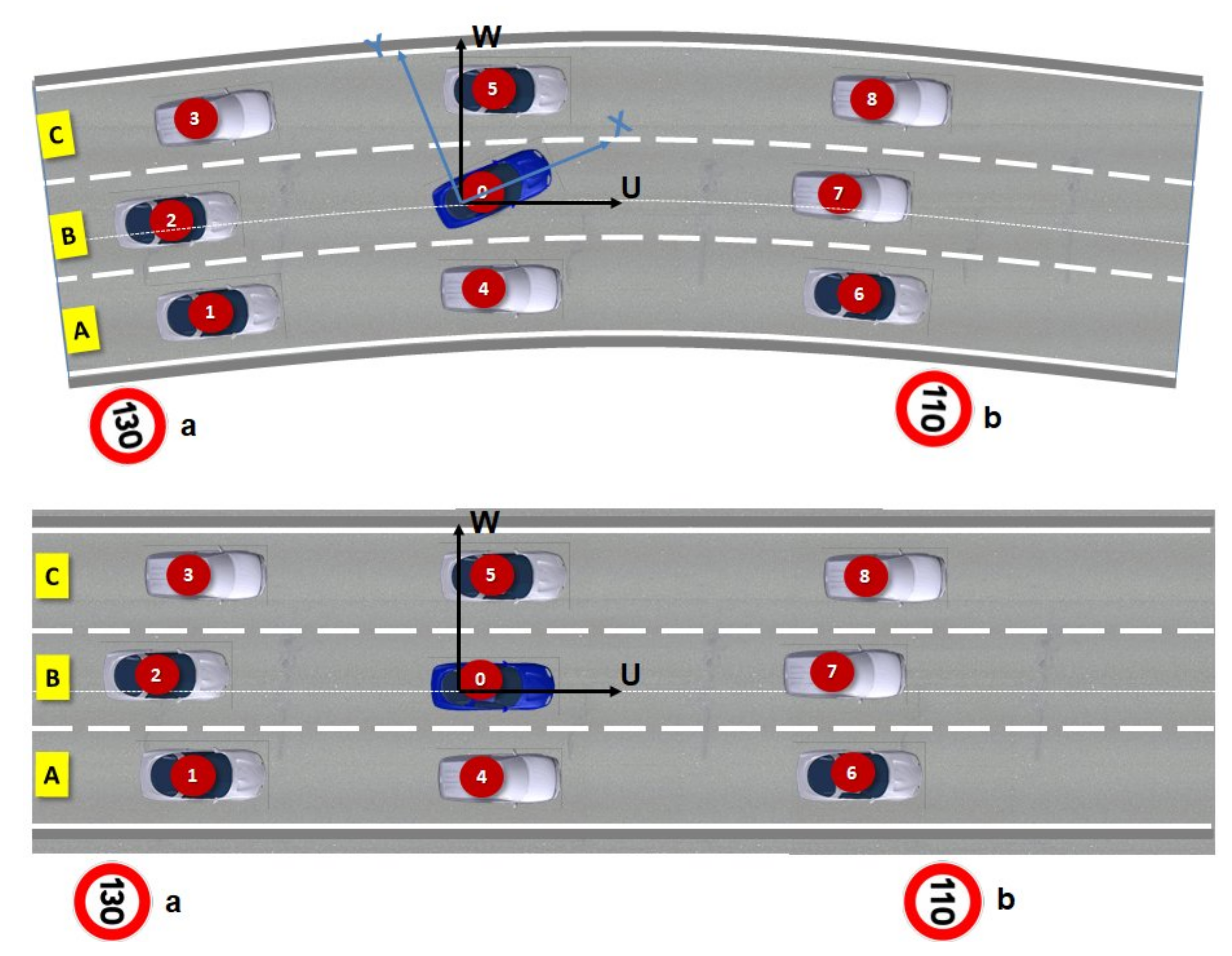
Appendix A.1. Computation of a Reference Space and Lane Coordinate System

In order to simplify the stages of trajectories computation and their associated risk level, a change of the referential is applied. We move from the XY Cartesian “world” perception reference (similar to Lambert coordinate 120 used by Global Navigation Satellite System (GNSS)) to a simpler and mostly linear UW local reference (Figure A1). The UW curvilinear lane coordinate system uses the same origin as the XY coordinate system of the ego-vehicle. In this new linear frame of reference, the U axis is parallel to the middle of each lane and the W axis is perpendicular to U. This UW environment is the easiest environment to use for trajectory calculations involving the ego-vehicle and the surrounding objects. This UW lane coordinate system and the XY ego-vehicle coordinate system are both shown in Figure A1. In the UW lane coordinate system, the lane centres have a constant W coordinate. Thus, the trajectories of the ego-vehicle and objects that target the lane centre can be represented by two sections: a transitional section (with variable W coordinates) and a permanent section (with constant W coordinates).
Computations with constant W coordinates are much easier and faster than computations in the XY lane geometry, which is usually (but not necessarily) based on a combination of lines, clothoid and circles [78]. After that, all trajectory computations of the ego-vehicle and objects will be performed in UW.
Figure A1. Perception of the environment (ego-vehicle, obstacles, traffic lanes and road markings) and passage of the real perception reference XY in the virtual path planning reference UW.
Applsci 11 06373 g0a1

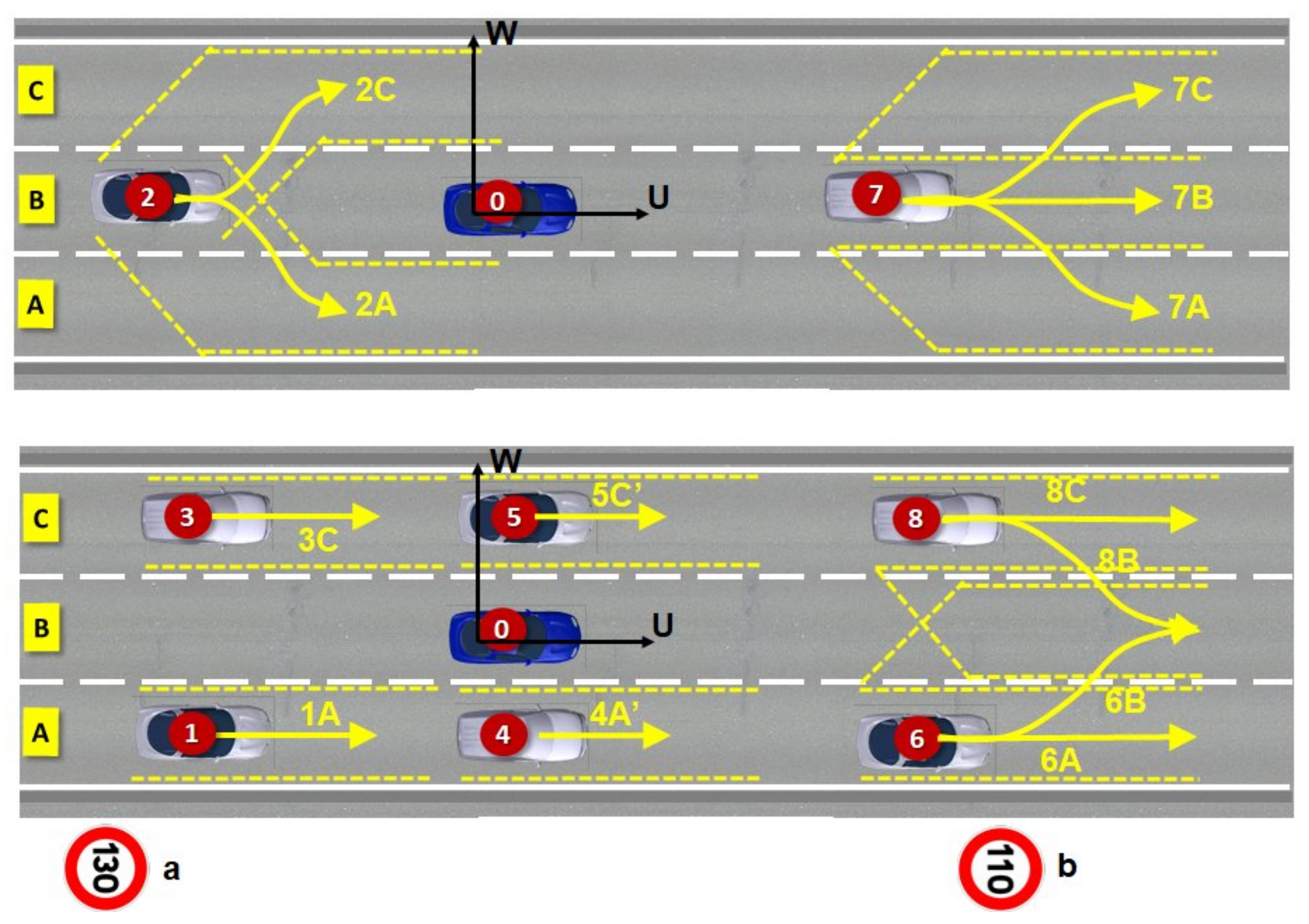
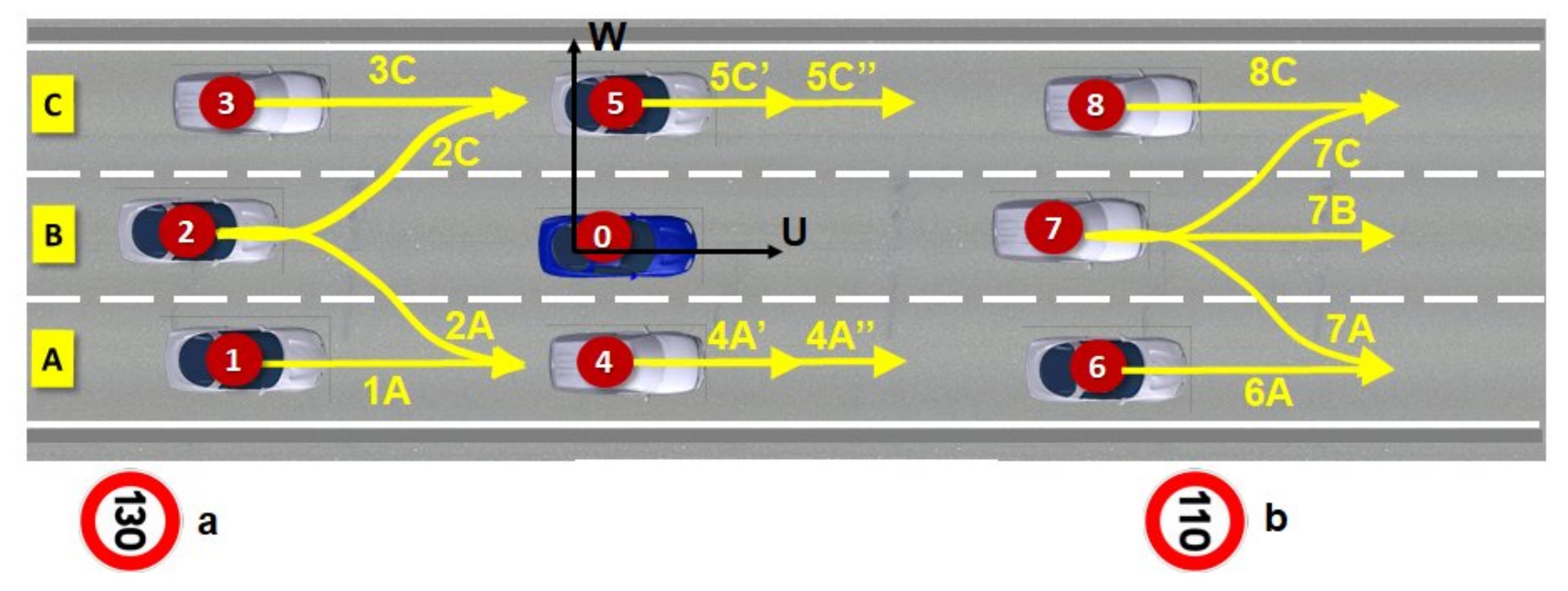
Appendix A.2. Computation of Trajectories for Both Objects and “Ghost” Vehicles

The “legal” and safe trajectories on the three lanes (A, B, and C) of the detected objects (objects numbered from 1 to 8) are predicted according to their dynamic state and traffic rules applicable to the current configuration. These trajectories are presented in Figure A2.
Added to this concept of trajectories generation over a temporal space, an extension is proposed and is presented in Figure A3 and shows the proposed concept of “model of mathematical area” generating the minimum and maximum trajectories (dotted line) reachable and admissible compared to an exemplary real trajectory (continuous line).
In order to be able to guarantee maximum safety even without a long-range perception capacity, the concept of the “ghost” vehicle has been proposed and developed as in Figure A3. The ghost vehicles are virtual objects added in the road environment in order to take into account the uncertainties and the possible risk over the limit of the ego-vehicle perception.
Figure A2. Prediction of possible trajectories for objects 1 to 8 depending on their position relatively to the ego-vehicle and traffic rules.
Applsci 11 06373 g0a2
Figure A3. Prediction of possible trajectories for objects 1 to 8 depending on their position relatively to the ego-vehicle and traffic rules.
Applsci 11 06373 g0a3
The next step will therefore predict “safe speed” profiles respecting traffic rules both for objects present in the environment close to the ego-vehicle (objects 1 to 8), and for “ghost” vehicles (I–VI) (Figure A4 and Figure A5).
Figure A4. Prediction of ghost trajectories (I–VI) as a function of the ego-vehicle current position including the minimum and maximum trajectory zones.
Applsci 11 06373 g0a4
Figure A5. Prediction of the speed profiles for objects (1–8) and “ghost” vehicles (I–VI) as a function of the ego-vehicle position (0).
Applsci 11 06373 g0a5

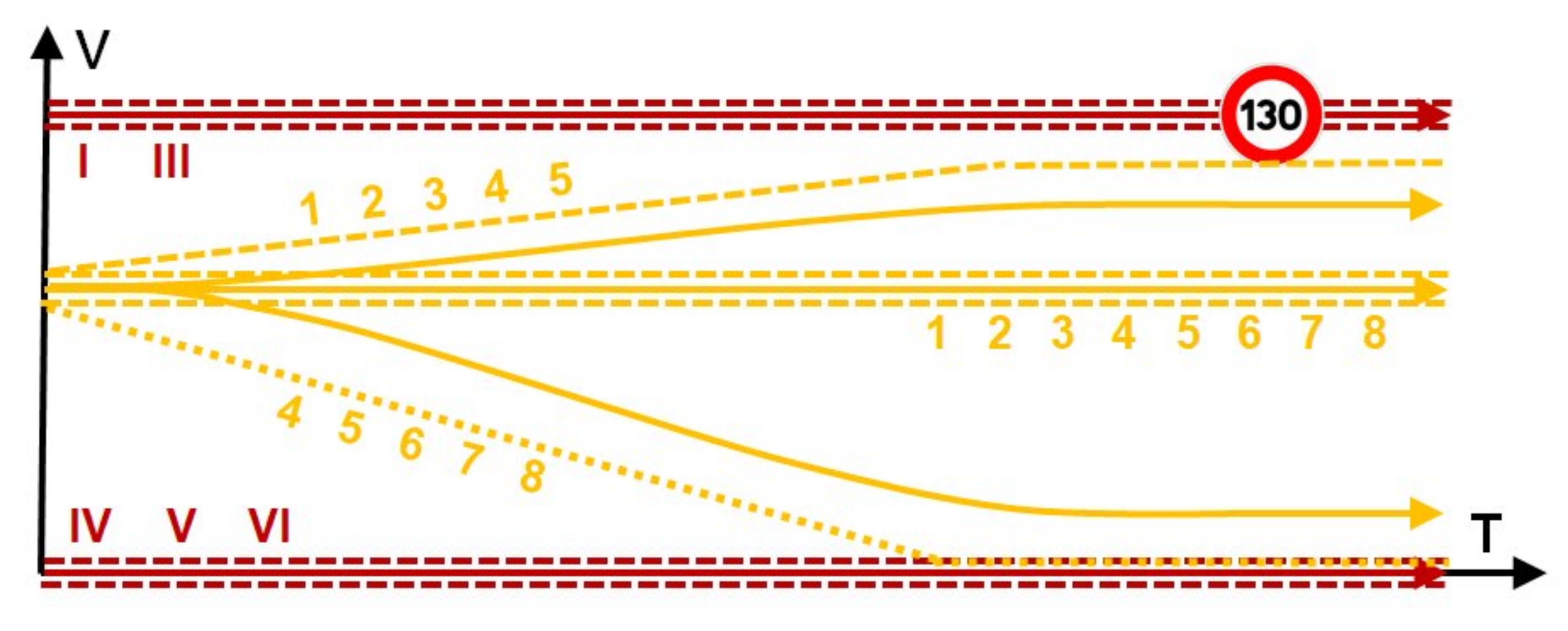
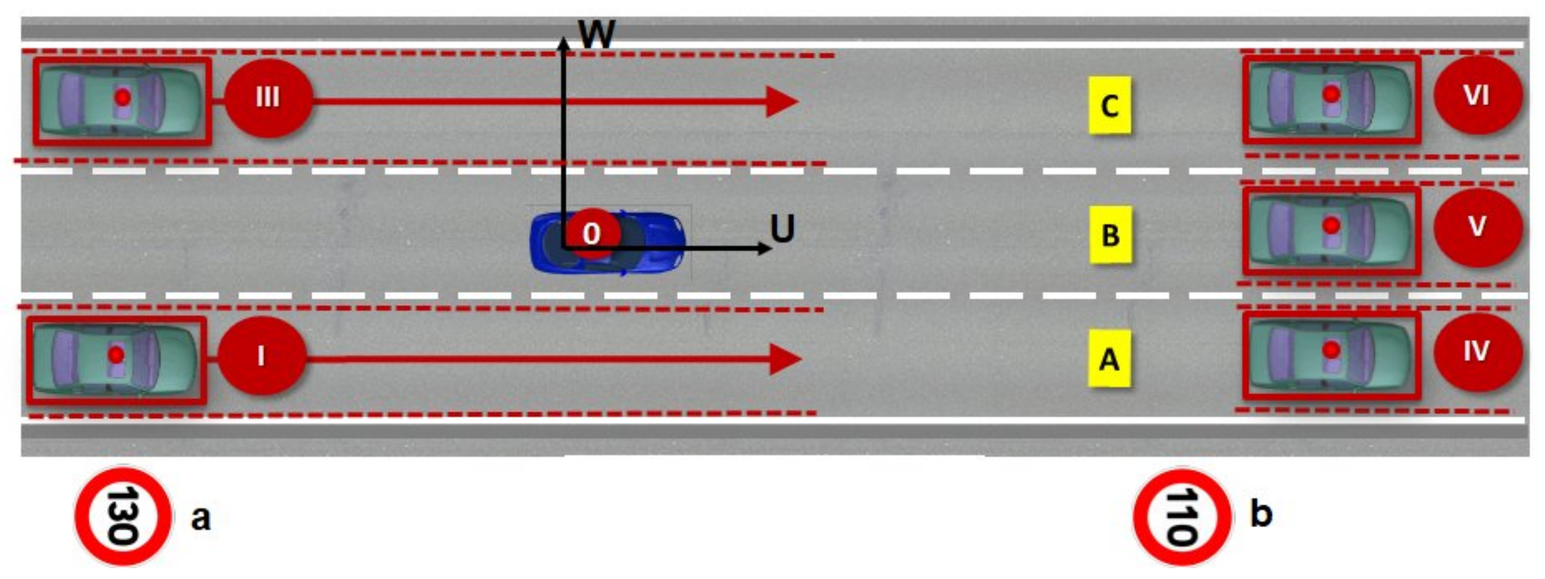
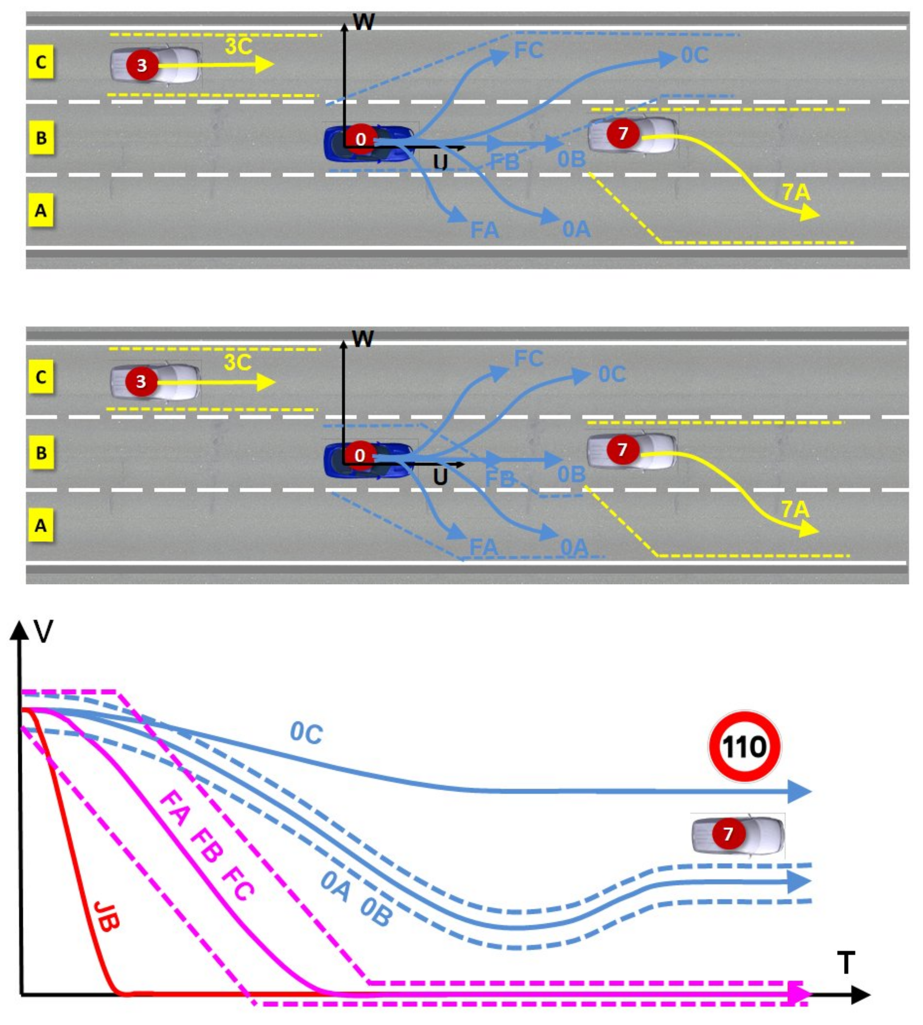
Appendix A.3. Prediction of Speed Profiles and Trajectories for the Ego-Vehicle

Once the trajectories of real and “ghost” objects have been predicted, we must now calculate the safe speed profiles which comply with the rules listed above for the ego-vehicle (0) and for the three traffic lanes (A–C). These speed profiles for the ego-vehicle must meet the constraints of intelligent speed adaptation and safe inter-distances keeping.
The computation of the reachable trajectories by the ego-vehicle is strongly based on the use of a module of environment perception (mainly the detection and tracking of obstacles and traffic lanes and road marking detection) and on the prediction of the object’s trajectory already presented in the previous section. In the existing literature on trajectory planning, two main types of algorithms exist: “sampling-based” algorithms and direct algorithms [79]. “Sampling-based” algorithms such as “sampling-based roadmap”, RRT algorithms or grid-based algorithms (space discretization) allow a universal approach by first generating random samples in the space of the trajectories, then evaluating these [40]. Direct algorithms, such as algorithms based on expert systems, potential or control fields, offer an application-specific approach that directly takes into account all the driving aspects in the generation of a trajectory, without the need for an assessment step. Direct algorithms find more optimal solutions and require fewer calculations than “sampling-based” algorithms. “Sampling-based” algorithms solve complex problems that direct algorithms are struggling to solve. A recent overview of these methods is presented in [80].
In our case, the “safe decision” module (from a traffic rule point of view) combines direct trajectory planning and a “sampling-based” algorithm. The “direct calculations” part is used for longitudinal maneuvers and for calculating the speed profiles of the ego-vehicle. The direct calculations are simple and accurate in the case of the use of continuous variables, such as the longitudinal speed from zero to the maximum speed, or the longitudinal acceleration going from extreme braking to strong acceleration. Calculations using the “sampling-based” approach are used for lateral maneuvers, which are discrete by nature. This is mainly due to the structure of the traffic lanes. In the current implementation of the decision module, only the trajectories centered towards the middle of the lanes are calculated. Figure A5 shows the generation of 7 possible speed profiles for the ego-vehicle, both longitudinal and lateral. These profiles are broken down into 3 categories.
  • The first corresponds to normal vehicle operation (0A, 0B, 0C).
  • The second takes into account the singular situations of breakdown and failure of an ego-vehicle embedded system (FA, FB, FC). The safety speed profiles generated in this case (F for failure) must allow stopping safely the ego-vehicle taking into account all the users.
  • The last category corresponds to a situation of safe reaction to a dangerous event requiring the use of a safety braking system or a collision requiring an emergency braking system (JB). This can occur when an unequipped vehicle does not respect traffic and human rules.
The categories 2 and 3 are “automated emergency mode” of the ADS module and represent a significant innovation in ADS. This emergency mode will be addressed and explained in more detail in the next section. In Figure A6, the zone/envelope model of minimum and maximum achievable speed for the trajectories 0A, 0B, FA, FB and FC is also generated.
Figure A6. Generation of the seven speed profiles (normal, failure, emergency braking) for the ego-vehicle.
Applsci 11 06373 g0a6
The decision module first calculates the speed profiles before calculating the paths. This approach is opposed to the classic “path-speed” decomposition approach [81]. In order to generate the velocity and acceleration profiles, a set of equations are implemented [64]. These equations apply the constraints related to the limits of the various parameters impacting the dynamics of the ego-vehicle (friction limits (G), human limits (H), and system limits (I)) depending on the infrastructure, objects in the environment, and “ghost” vehicles modeling the safety limit cases imposed by the limits of the electronic horizon provided by the perception stage. These limits are related to the vehicle capacity, the driver’s behavior and driving style, and the limits of the perception and control modules.
The different implemented equations have for the main task to give the conditions on the transient section for a speed profile as a function of the longitudinal friction, the human limits, and the system limits. The maximum speed is obtained from the target speed (possibly defined by the human driver) and the maximum speed for which the system is designed. For the speed profiles in “emergency” mode (FA, FB and FC), the target speed recommended will be defined in Section 4.
Moreover, constraints both on the speed profiles and on the paths of the ego-vehicle are taken into account. In the case of an overtaking maneuver, it will be necessary to adapt both the speed profile and the path. As for a target tracking maneuver, changing lanes also involves the use of a safety distance. This safety distance prevents an accident if an obstacle (in the current lane or the target lane) performs emergency braking.
It is important to quote that equations are developed in order to take into account some constraints related to the slope of the road, the target speed profile and the acceleration in order to respect the safety distance during all the maneuvers.

Appendix A.4. Evaluation and Selection of Trajectories for ADS

As we have seen previously, the decision module directly integrates most of the legal and regulatory safety aspects in the generation of the ego-vehicle speed profiles and the ego-vehicle trajectories. The speed profiles, respecting the safety constraints, are obtained by taking the minimum of the speed profiles with respect to the constraints applied in the computation of the prediction of speed profiles and trajectories for the ego-vehicle. The legal safety trajectories are found by taking the maximum (absolute values) of the trajectories relative to the following constraints: comfort, the maximum slope of the trajectories, target speed profiles, and accelerations. This gives seven speed profiles and seven trajectories for the ego-vehicle: 0A, 0B and 0C for normal system operation, FA, FB, FC and JB for operation in “emergency” mode (including “collision mitigation” and “emergency braking”). The objective of the evaluation stage will be to evaluate these seven trajectories on the aspects which were not taken into account in the previous stage of trajectories generation.
A performance cost is assigned to each of the remaining safety aspects. The cost of performance is binary (for instance, non-physical trajectories are immediately rejected), except for collisions with obstacles. In this case, the cost is proportional to the impact speed of the collision. This allows choosing the trajectory with a minimal impact in situations where an accident cannot be avoided. In the trajectory generation step, only “ghost” vehicles and frontal objects were taken into account. The trajectory assessment stage also considers the prediction of both the “ghosts” and “vehicles” trajectories present at the rear of the ego vehicle and on the adjacent lanes. This assessment step verifies that the speed and speed profile of the ego-vehicle allow “ghost” vehicles to brake until the ego-vehicle speed with a reasonable deceleration. The assessment stage also checks that the vehicles at the rear and on the sides do not need to brake during an ego-vehicle maneuver. The evaluation only applies to lane change trajectories 0A, 0C, FA and FC, and not to lane-keeping trajectories 0B, FB and JB. In the current lane of the ego-vehicle, it stays the priority vehicle on the “ghosts” and “obstacles” vehicles in both rear and adjacent lanes.
The evaluation step also takes into account the type of target lane and the associated road markings to validate or not the lane change trajectories 0A, 0C, FA and FC. Moreover, in normal driving, the 0A and 0C trajectories should only target accessible lanes that do not have continuous lane markings. On the other hand, the “emergency” trajectories (FA and FC) can operate on an emergency stop lane or on a normal lane, and the ego vehicle can then cross continuous lane markings. Indeed, a lane change towards an emergency stop lane is preferable to a collision with another vehicle. This maneuver is a priority safety maneuver.
The application of each rule greatly reduces the trajectory solutions space. For instance, the “traffic” rules may exclude the possibility of lane changing, the “human” rules limit the ego-vehicle speed, and the “system” rules limit the deceleration and acceleration capabilities of the ego-vehicle. However, after this evaluation stage, a minimum of at least one trajectory must exist to allow the safe evolution of the ego vehicle. In the worst case, an emergency trajectory is generated.

References

  1. Tsugawa, S.; Kitoh, K.; Fujii, H.; Koide, K.; Harada, T.; Miura, K.; Yasunobu, S.; Wakabayashi, Y. Info-Mobility: A Concept for Advanced Automotive Functions toward the 21st Century; Technical Report; SAE Technical Paper; SAE International: Pittsburgh, PA, USA, 1991. [Google Scholar]
  2. Maurer, M.; Christian Gerdes, J.; Lenz, B.; Winner, H. Autonomous Driving: Technical, Legal and Social Aspects; Springer Nature: Berlin/Heidelberg, Germany, 2016. [Google Scholar]
  3. Dickmann, J.; Klappstein, J.; Hahn, M.; Appenrodt, N.; Bloecher, H.L.; Werber, K.; Sailer, A. Automotive radar the key technology for autonomous driving: From detection and ranging to environmental understanding. In Proceedings of the 2016 IEEE Radar Conference (RadarConf), Philadelphia, PA, USA, 1–6 May 2016; pp. 1–6. [Google Scholar]
  4. Wu, B.F.; Lee, T.T.; Chang, H.H.; Jiang, J.J.; Lien, C.N.; Liao, T.Y.; Perng, J.W. GPS navigation based autonomous driving system design for intelligent vehicles. In Proceedings of the 2007 IEEE International Conference on Systems, Man and Cybernetics, Montréal, QC, Canada, 7–10 October 2007; pp. 3294–3299. [Google Scholar]
  5. Baber, J.; Kolodko, J.; Noel, T.; Parent, M.; Vlacic, L. Cooperative autonomous driving: Intelligent vehicles sharing city roads. IEEE Robot. Autom. Mag. 2005, 12, 44–49. [Google Scholar] [CrossRef] [Green Version]
  6. Schwarting, W.; Alonso-Mora, J.; Rus, D. Planning and decision-making for autonomous vehicles. Annu. Rev. Control. Robot. Auton. Syst. 2018, 1, 187–210. [Google Scholar] [CrossRef]
  7. Canny, J.; Reif, J. New lower bound techniques for robot motion planning problems. In Proceedings of the 28th Annual Symposium on Foundations of Computer Science (sfcs 1987), Los Angeles, CA, USA, 12–14 October 1987; pp. 49–60. [Google Scholar]
  8. DARPA. Darpa Urban Challenge. 2007. Available online: http://archive.darpa.mil/grandchallenge/ (accessed on 7 July 2021).
  9. Urmson, C.; Anhalt, J.; Bagnell, D.; Baker, C.; Bittner, R.; Clark, M.; Dolan, J.; Duggins, D.; Galatali, T.; Geyer, C.; et al. Autonomous driving in urban environments: Boss and the urban challenge. J. Field Robot. 2008, 25, 425–466. [Google Scholar] [CrossRef] [Green Version]
  10. Bacha, A.; Bauman, C.; Faruque, R.; Fleming, M.; Terwelp, C.; Reinholtz, C.; Hong, D.; Wicks, A.; Alberi, T.; Anderson, D.; et al. Odin: Team victortango’s entry in the darpa urban challenge. J. Field Robot. 2008, 25, 467–492. [Google Scholar] [CrossRef]
  11. Hülsen, M.; Zöllner, J.M.; Weiss, C. Traffic intersection situation description ontology for advanced driver assistance. In Proceedings of the 2011 IEEE Intelligent Vehicles Symposium (IV), Baden-Baden, Germany, 5–9 June 2011; pp. 993–999. [Google Scholar]
  12. Zhao, L.; Ichise, R.; Yoshikawa, T.; Naito, T.; Kakinami, T.; Sasaki, Y. Ontology-based decision making on uncontrolled intersections and narrow roads. In Proceedings of the 2015 IEEE Intelligent Vehicles Symposium (IV), Seoul, Korea, 28 June–1 July 2015; pp. 83–88. [Google Scholar]
  13. Kohlhaas, R.; Hammann, D.; Schamm, T.; Zöllner, J.M. Planning of high-level maneuver sequences on semantic state spaces. In Proceedings of the 2015 IEEE 18th International Conference on Intelligent Transportation Systems, Gran Canaria, Spain, 15–18 September 2015; pp. 2090–2096. [Google Scholar]
  14. Kochenderfer, M.J. Decision Making Under Uncertainty: Theory and Application; MIT Press: Cambridge, MA, USA, 2015. [Google Scholar]
  15. Brechtel, S.; Gindele, T.; Dillmann, R. Probabilistic decision-making under uncertainty for autonomous driving using continuous POMDPs. In Proceedings of the 17th International IEEE Conference on Intelligent Transportation Systems (ITSC), The Hague, The Netherlands, 24–26 September 2014; pp. 392–399. [Google Scholar]
  16. Liu, W.; Kim, S.W.; Pendleton, S.; Ang, M.H. Situation-aware decision making for autonomous driving on urban road using online POMDP. In Proceedings of the 2015 IEEE Intelligent Vehicles Symposium (IV), Seoul, Korea, 28 June–1 July 2015; pp. 1126–1133. [Google Scholar]
  17. Hubmann, C.; Becker, M.; Althoff, D.; Lenz, D.; Stiller, C. Decision making for autonomous driving considering interaction and uncertain prediction of surrounding vehicles. In Proceedings of the 2017 IEEE Intelligent Vehicles Symposium (IV), Los Angeles, CA, USA, 11–14 June 2017; pp. 1671–1678. [Google Scholar]
  18. Werling, M.; Ziegler, J.; Kammel, S.; Thrun, S. Optimal trajectory generation for dynamic street scenarios in a frenet frame. In Proceedings of the 2010 IEEE International Conference on Robotics and Automation, Anchorage, AK, USA, 3–8 May 2010; pp. 987–993. [Google Scholar]
  19. Xu, W.; Pan, J.; Wei, J.; Dolan, J.M. Motion planning under uncertainty for on-road autonomous driving. In Proceedings of the 2014 IEEE International Conference on Robotics and Automation (ICRA), Hong Kong, China, 31 May–5 June 2014; pp. 2507–2512. [Google Scholar]
  20. Damerow, F.; Eggert, J. Risk-aversive behavior planning under multiple situations with uncertainty. In Proceedings of the 2015 IEEE 18th International Conference on Intelligent Transportation Systems, Las Palmas de Gran Canaria, Spain, 15–18 September 2015; pp. 656–663. [Google Scholar]
  21. Codevilla, F.; Müller, M.; López, A.; Koltun, V.; Dosovitskiy, A. End-to-end driving via conditional imitation learning. In Proceedings of the 2018 IEEE International Conference on Robotics and Automation (ICRA), Brisbane, Australia, 21–25 May 2018; pp. 4693–4700. [Google Scholar]
  22. Chen, J.; Yuan, B.; Tomizuka, M. Deep imitation learning for autonomous driving in generic urban scenarios with enhanced safety. arXiv 2019, arXiv:1903.00640. [Google Scholar]
  23. Hoel, C.J.; Driggs-Campbell, K.; Wolff, K.; Laine, L.; Kochenderfer, M.J. Combining planning and deep reinforcement learning in tactical decision making for autonomous driving. IEEE Trans. Intell. Veh. 2019, 5, 294–305. [Google Scholar] [CrossRef] [Green Version]
  24. Dijkstra, E.W. A note on two problems in connexion with graphs. Numer. Math. 1959, 1, 269–271. [Google Scholar] [CrossRef] [Green Version]
  25. Hart, P.E.; Nilsson, N.J.; Raphael, B. A formal basis for the heuristic determination of minimum cost paths. IEEE Trans. Syst. Sci. Cybern. 1968, 4, 100–107. [Google Scholar] [CrossRef]
  26. Dolgov, D.; Thrun, S.; Montemerlo, M.; Diebel, J. Practical search techniques in path planning for autonomous driving. Ann Arbor 2008, 1001, 18–80. [Google Scholar]
  27. Nash, A.; Daniel, K.; Koenig, S.; Felner, A. Thetaˆ*: Any-Angle Path Planning on Grids; AAAI: Los Angeles, CA, USA, 2007; Volume 7, pp. 1177–1183. [Google Scholar]
  28. Ferguson, D.; Stentz, A. Using interpolation to improve path planning: The Field D* algorithm. J. Field Robot. 2006, 23, 79–101. [Google Scholar] [CrossRef] [Green Version]
  29. Koenig, S.; Likhachev, M. D* lite. In Proceedings of the National Conference on Artificial Intelligence (AAAI), Edmonton, AB, Canada, 28 July–1 August 2002. [Google Scholar]
  30. Artunedo, A.; Villagra, J.; Godoy, J.; del Castillo, M.D. Motion planning approach considering localization uncertainty. IEEE Trans. Veh. Technol. 2020, 69, 5983–5994. [Google Scholar] [CrossRef]
  31. Lambert, A.; Gruyer, D. Safe path planning in an uncertain-configuration space. In Proceedings of the 2003 IEEE International Conference on Robotics and Automation (Cat. No. 03CH37422), Taipei, Taiwan, 14–19 September 2003; Volume 3, pp. 4185–4190. [Google Scholar]
  32. Kavraki, L.E.; Kolountzakis, M.N.; Latombe, J.C. Analysis of probabilistic roadmaps for path planning. IEEE Trans. Robot. Autom. 1998, 14, 166–171. [Google Scholar] [CrossRef] [Green Version]
  33. LaValle, S.M. Rapidly-Exploring Random Trees: A New Tool for Path Planning; Technical Report TR 98-11; Iowa State University: Ames, IA, USA, 1998. [Google Scholar]
  34. Ma, L.; Xue, J.; Kawabata, K.; Zhu, J.; Ma, C.; Zheng, N. Efficient sampling-based motion planning for on-road autonomous driving. IEEE Trans. Intell. Transp. Syst. 2015, 16, 1961–1976. [Google Scholar] [CrossRef]
  35. Feraco, S.; Luciani, S.; Bonfitto, A.; Amati, N.; Tonoli, A. A local trajectory planning and control method for autonomous vehicles based on the RRT algorithm. In Proceedings of the 2020 AEIT International Conference of Electrical and Electronic Technologies for Automotive (AEIT AUTOMOTIVE), Turin, Italy, 18–20 November 2020; pp. 1–6. [Google Scholar]
  36. Ferguson, D.; Stentz, A. Anytime rrts. In Proceedings of the 2006 IEEE/RSJ International Conference on Intelligent Robots and Systems, Beijing, China, 9–15 October 2006; pp. 5369–5375. [Google Scholar]
  37. Kuffner, J.J.; LaValle, S.M. RRT-connect: An efficient approach to single-query path planning. In Proceedings of the 2000 ICRA, Millennium Conference. IEEE International Conference on Robotics and Automation, Symposia Proceedings (Cat. No. 00CH37065), San Francisco, CA, USA, 24–28 April 2000; Volume 2, pp. 995–1001. [Google Scholar]
  38. Ferguson, D.; Kalra, N.; Stentz, A. Replanning with rrts. In Proceedings of the 2006 IEEE International Conference on Robotics and Automation, ICRA 2006, Orlando, FL, USA, 15–19 May 2006; pp. 1243–1248. [Google Scholar]
  39. Karaman, S.; Frazzoli, E. Optimal kinodynamic motion planning using incremental sampling-based methods. In Proceedings of the 49th IEEE Conference on Decision and Control (CDC), Atlanta, GA, USA, 15–17 December 2010; pp. 7681–7687. [Google Scholar]
  40. Karaman, S.; Frazzoli, E. Sampling-based algorithms for optimal motion planning. Int. J. Robot. Res. 2011, 30, 846–894. [Google Scholar] [CrossRef]
  41. Volpe, R.; Khosla, P. Manipulator control with superquadric artificial potential functions: Theory and experiments. IEEE Trans. Syst. Man Cybern. 1990, 20, 1423–1436. [Google Scholar] [CrossRef] [Green Version]
  42. Vadakkepat, P.; Tan, K.C.; Ming-Liang, W. Evolutionary artificial potential fields and their application in real time robot path planning. In Proceedings of the 2000 Congress on Evolutionary Computation, CEC00 (Cat. No. 00TH8512), La Jolla, CA, USA, 16–19 July 2000; Volume 1, pp. 256–263. [Google Scholar]
  43. Wolf, M.T.; Burdick, J.W. Artificial potential functions for highway driving with collision avoidance. In Proceedings of the 2008 IEEE International Conference on Robotics and Automation, Pasadena, CA, USA, 19–23 May 2008; pp. 3731–3736. [Google Scholar]
  44. Xu, Y.; Ma, Z.; Sun, J. Simulation of turning vehicles’ behaviors at mixed-flow intersections based on potential field theory. Transp. Transp. Dyn. 2019, 7, 498–518. [Google Scholar] [CrossRef]
  45. Koren, Y.; Borenstein, J. Potential field methods and their inherent limitations for mobile robot navigation. In Proceedings of International Conference on Robotics and Automation, Sacramento, CA, USA, 7–12 April 1991; pp. 1398–1404. [Google Scholar]
  46. Caijing, X.; Hui, C. A research on local path planning for antonomous vehicles based on improved APF method. Automot. Eng. 2013, 35, 808. [Google Scholar]
  47. Park, M.G.; Lee, M.C. A new technique to escape local minimum in artificial potential field based path planning. KSME Int. J. 2003, 17, 1876–1885. [Google Scholar] [CrossRef]
  48. Wang, P.; Gao, S.; Li, L.; Sun, B.; Cheng, S. Obstacle avoidance path planning design for autonomous driving vehicles based on an improved artificial potential field algorithm. Energies 2019, 12, 2342. [Google Scholar] [CrossRef] [Green Version]
  49. Le Gouguec, A.; Kemeny, A.; Berthoz, A.; Merienne, F. Artificial Potential Field Simulation Framework for Semi-Autonomous Car Conception. In Proceedings of the Driving Simulation Conference, Stuttgart, Germany, 6–8 September 2017; pp. 20–22. [Google Scholar]
  50. Quinlan, S.; Khatib, O. Elastic bands: Connecting path planning and control. In Proceedings of the IEEE International Conference on Robotics and Automation, Atlanta, GA, USA, 2–6 May 1993; pp. 802–807. [Google Scholar]
  51. Hilgert, J.; Hirsch, K.; Bertram, T.; Hiller, M. Emergency path planning for autonomous vehicles using elastic band theory. In Proceedings of the 2003 IEEE/ASME International Conference on Advanced Intelligent Mechatronics (AIM 2003), Kobe, Japan, 20–24 July 2003; Volume 2, pp. 1390–1395. [Google Scholar]
  52. Ararat, Ö.; Güvenç, B.A. Development of a collision avoidance algorithm using elastic band theory. IFAC Proc. Vol. 2008, 41, 8520–8525. [Google Scholar] [CrossRef]
  53. Song, X.; Cao, H.; Huang, J. Influencing factors research on vehicle path planning based on elastic bands for collision avoidance. SAE Int. J. Passeng.-Cars-Electron. Electr. Syst. 2012, 5, 625–637. [Google Scholar] [CrossRef]
  54. Song, X.; Cao, H.; Huang, J. Vehicle path planning in various driving situations based on the elastic band theory for highway collision avoidance. Proc. Inst. Mech. Eng. Part J. Automob. Eng. 2013, 227, 1706–1722. [Google Scholar] [CrossRef]
  55. Polack, P.; Altché, F.; d’Andréa Novel, B.; de La Fortelle, A. The kinematic bicycle model: A consistent model for planning feasible trajectories for autonomous vehicles? In Proceedings of the 2017 IEEE Intelligent Vehicles Symposium (IV), Los Angeles, CA, USA, 11–17 June 2017; pp. 812–818. [Google Scholar]
  56. Normey-Rico, J.E.; Alcalá, I.; Gómez-Ortega, J.; Camacho, E.F. Mobile robot path tracking using a robust PID controller. Control. Eng. Pract. 2001, 9, 1209–1214. [Google Scholar] [CrossRef]
  57. Samuel, M.; Hussein, M.; Mohamad, M.B. A review of some pure-pursuit based path tracking techniques for control of autonomous vehicle. Int. J. Comput. Appl. 2016, 135, 35–38. [Google Scholar] [CrossRef]
  58. Buehler, M.; Iagnemma, K.; Singh, S. The 2005 DARPA Grand Challenge: The Great Robot Race; Springer: Berlin/Heidelberg, Germany, 2007; Volume 36. [Google Scholar]
  59. Hoffmann, G.M.; Tomlin, C.J.; Montemerlo, M.; Thrun, S. Autonomous automobile trajectory tracking for off-road driving: Controller design, experimental validation and racing. In Proceedings of the 2007 American Control Conference, New York, NY, USA, 9–13 July 2007; pp. 2296–2301. [Google Scholar]
  60. Makarem, L.; Gillet, D. Model predictive coordination of autonomous vehicles crossing intersections. In Proceedings of the 16th International IEEE Conference on Intelligent Transportation Systems (ITSC 2013), The Hague, The Netherlands, 6–9 October 2013; pp. 1799–1804. [Google Scholar]
  61. Campos, G.R.; Falcone, P.; Wymeersch, H.; Hult, R.; Sjöberg, J. Cooperative receding horizon conflict resolution at traffic intersections. In Proceedings of the 53rd IEEE Conference on Decision and Control, Los Angeles, CA, USA, 15–17 December 2014; pp. 2932–2937. [Google Scholar]
  62. Wang, H.; Liu, B.; Ping, X.; An, Q. Path tracking control for autonomous vehicles based on an improved MPC. IEEE Access 2019, 7, 161064–161073. [Google Scholar] [CrossRef]
  63. Kapania, N.R.; Gerdes, J.C. Design of a feedback-feedforward steering controller for accurate path tracking and stability at the limits of handling. Veh. Syst. Dyn. 2015, 53, 1687–1704. [Google Scholar] [CrossRef] [Green Version]
  64. Vanholme, B.; Gruyer, D.; Lusetti, B.; Glaser, S.; Mammar, S. Highly automated driving on highways based on legal safety. IEEE Trans. Intell. Transp. Syst. 2012, 14, 333–347. [Google Scholar] [CrossRef]
  65. Trustonomy Project. 2020. Available online: https://h2020-trustonomy.eu/ (accessed on 7 July 2021).
  66. Resende, P.; Pollard, E.; Li, H.; Nashashibi, F. ABV-A Low Speed Automation Project to Study the Technical Feasibility of Fully Automated Driving. In Proceedings of the Workshop PAMM, Kumamoto, Japan, 9–10 November 2013. [Google Scholar]
  67. Gruyer, D.; Magnier, V.; Hamdi, K.; Claussmann, L.; Orfila, O.; Rakotonirainy, A. Perception, information processing and modeling: Critical stages for autonomous driving applications. Annu. Rev. Control. 2017, 44, 323–341. [Google Scholar] [CrossRef]
  68. Caballero, W.N.; Ríos Insua, D.; Banks, D. Decision support issues in automated driving systems. Int. Trans. Oper. Res. 2021. Available online: http://xxx.lanl.gov/abs/https://onlinelibrary.wiley.com/doi/pdf/10.1111/itor.12936 (accessed on 7 July 2021). [CrossRef]
  69. The IEEE Global Initiative on Ethics of Autonomous and Intelligent Systems. Available online: https://standards.ieee.org/content/dam/ieee-standards/standards/web/documents/other/ead1e_embedding_values.pdf (accessed on 7 July 2021).
  70. Sattel, T.; Brandt, T. Ground vehicle guidance along collision-free trajectories using elastic bands. In Proceedings of the 2005 American Control Conference, Portland, OR, USA, 10 June 2005; pp. 4991–4996. [Google Scholar]
  71. Perrollaz, M.; Labayrade, R.; Gruyer, D.; Lambert, A.; Aubert, D. Proposition of generic validation criteria using stereo-vision for on-road obstacle detection. Int. J. Robot. Autom. 2014, 29, 65–87. [Google Scholar] [CrossRef]
  72. Gruyer, D.; Cord, A.; Belaroussi, R. Vehicle detection and tracking by collaborative fusion between laser scanner and camera. In Proceedings of the 2013 IEEE/RSJ International Conference on Intelligent Robots and Systems, Tokyo, Japan, 3–7 November 2013; pp. 5207–5214. [Google Scholar]
  73. Gruyer, D.; Demmel, S.; Magnier, V.; Belaroussi, R. Multi-hypotheses tracking using the Dempster–Shafer theory, application to ambiguous road context. Inf. Fusion 2016, 29, 40–56. [Google Scholar] [CrossRef] [Green Version]
  74. Revilloud, M.; Gruyer, D.; Pollard, E. An improved approach for robust road marking detection and tracking applied to multi-lane estimation. In Proceedings of the 2013 IEEE Intelligent Vehicles Symposium (IV), Gold Coast City, Australia, 23–26 June 2013; pp. 783–790. [Google Scholar]
  75. Revilloud, M.; Gruyer, D.; Rahal, M.C. A new multi-agent approach for lane detection and tracking. In Proceedings of the 2016 IEEE International Conference on Robotics and Automation (ICRA), Stockholm, Sweden, 16–21 May 2016; pp. 3147–3153. [Google Scholar]
  76. Ndjeng, A.N.; Gruyer, D.; Glaser, S.; Lambert, A. Low cost IMU–Odometer–GPS ego localization for unusual maneuvers. Inf. Fusion 2011, 12, 264–274. [Google Scholar] [CrossRef]
  77. Gruyer, D.; Belaroussi, R.; Revilloud, M. Accurate lateral positioning from map data and road marking detection. Expert Syst. Appl. 2016, 43, 1–8. [Google Scholar] [CrossRef]
  78. Rajamani, R. Vehicle Dynamics and Control; Springer Science & Business Media: New York, NY, USA, 2011. [Google Scholar]
  79. LaValle, S.M. Planning Algorithms; Cambridge University Press: Cambridge, UK, 2006. [Google Scholar]
  80. Claussmann, L.; Revilloud, M.; Gruyer, D.; Glaser, S. A review of motion planning for highway autonomous driving. IEEE Trans. Intell. Transp. Syst. 2019, 21, 1826–1848. [Google Scholar] [CrossRef] [Green Version]
  81. Kant, K.; Zucker, S.W. Toward efficient trajectory planning: The path-velocity decomposition. Int. J. Robot. Res. 1986, 5, 72–89. [Google Scholar] [CrossRef]
Figure 1. Perception and decision levels.
Applsci 11 06373 g001
Figure 2. Similarity between human and machine driving task [67].
Applsci 11 06373 g002
Figure 3. Archimate global architecture of the Automated Decision-Support module.
Applsci 11 06373 g003
Figure 4. Mode transitions.
Applsci 11 06373 g004
Figure 5. Classic Elastic Band.
Applsci 11 06373 g005
Figure 6. Improved Elastic Band.
Applsci 11 06373 g006
Figure 7. Abrupt change of velocity.
Applsci 11 06373 g007
Figure 8. Abrupt change of orientation.
Applsci 11 06373 g008
Figure 9. Potential of boundary and lane.
Applsci 11 06373 g009
Figure 10. New trajectory in non-driving area.
Applsci 11 06373 g010
Figure 11. Pro-SiVIC, a generic and physically realistic simulation platform for sensors, vehicles, and environment. Right: Co-Pilot application.
Applsci 11 06373 g011
Figure 12. A dedicated real prototype for highly automated driving applications.
Applsci 11 06373 g012
Figure 13. “Approaching a speed limit” scenario.
Applsci 11 06373 g013
Figure 14. “Approaching a vehicle or a ghost zone” scenario.
Applsci 11 06373 g014
Figure 15. “Following target” scenario, with a change in speed and lane.
Applsci 11 06373 g015
Figure 16. “Overtaking a target and returning to the original lane” scenario with Pro-SiVIC platform.
Applsci 11 06373 g016
Figure 17. Repulsive potential of obstacles.
Applsci 11 06373 g017
Figure 18. Different scenarios of the ego-vehicle passing an intersection with a moving obstacle.
Applsci 11 06373 g018aApplsci 11 06373 g018b
Figure 19. Example of critical scenarios.
Applsci 11 06373 g019
Figure 20. Trajectories forthe two critical scenarios needed emergency behaviors.
Applsci 11 06373 g020
Figure 21. Parameters of ego vehicle in first scenario: distance to obstacle (left), speed (middle) and steering angle (right).
Applsci 11 06373 g021
Figure 22. Parameters of ego vehicle in second scenario: distance to obstacle (left), speed (middle) and steering angle (right).
Applsci 11 06373 g022
Table 1. Parameters adopted in the simulations.
NotationsDescriptionValue
Indices
Δ t interval of time step0.25 (s)
wwidth of the road4 (m)
llength of the vehicle4 (m)
hwidth of the vehicle2.5 (m)
v i n i t i a l initial velocity of the vehicle10 (m/s)
θ i n i t i a l initial orientation of the vehicle0 (°)
k i n t e r n a l strength of internal force1
F o r c e _ l i m i t condition of equilibrium1 × 10−3
Problem parameters
pidentify the acting area of boundary force5 (m)
k l a n e strength of external force from the lane0.02
k b o u n d a r y strength of external force from the boundary0.002
k o b s strength of external force from the obstacles5
Nnumber of the nodes in exploring trajectory10
I t m a x maximal number of iterations20
State variables
k i the array of the parameters of the forces in the non-driving area at iteration i[0,1]
Publisher’s Note: MDPI stays neutral with regard to jurisdictional claims in published maps and institutional affiliations.

