Improved Generalized Cross-Validation and Unbiased Predictive Risk Estimator Methods Using the RGSVD: Application to Inversion of Potential Field Data

Abstract

The inversion of potential field data has widely utilized the generalized cross-validation (GCV) and the unbiased predictive risk estimator (UPRE) methods to determine the regularization parameter. However, these two methods are time-consuming and it is difficult for them to determine the optimal linear search range including the optimal regularization. To solve these problems, this article improves the GCV and UPRE methods using the RGSVD (randomized generalized singular value decomposition) algorithm. The improved methods first use the randomized algorithm to compute an approximate generalized singular value decomposition (GSVD) with less computational time. Then, the optimal linear search range is determined based on the generalized singular values. Finally, the GCV and the UPRE functions are efficiently computed on the basis of the results from the RGSVD algorithm. In this way, the GCV and UPRE methods using the RGSVD algorithm are able to determine the optimal regularization parameter fast and effectively. One comparative test shows the effectiveness and efficiency of the GCV and the UPRE methods using the RGSVD algorithm.

1. Introduction

Various geological and geophysical problems can be solved by the inversion of potential field data [1,2]. Generally, the inversion of potential field data is an ill-posed problem, which means that this inversion is usually non-unique and unstable [3]. Tikhonov regularization [4] can solve ill-posed problems. Estimating an optimal regularization parameter is very significant for the Tikhonov regularization, e.g., [5]. In the literature, many methods have been introduced to determine an optimal regularization parameter, such as the Morozov discrepancy principle (MDP) method [6], the generalized cross-validation (GCV) method [7], the L-curve (LC) method [8], and the unbiased predictive risk estimator (UPRE) method [9].

Here, we focus on the GCV and the UPRE methods. The conjugate gradient (CG) method and generalized singular value decomposition (GSVD) can be used to compute the GCV and the UPRE functions in a linear search range to find the optimal regularization parameter. However, when using the CG method, the process is time-consuming, and it is difficult to determine the optimal linear search range including the optimal regularization parameter. When using the GSVD, the optimal linear search range can be determined by analyzing the spectrum (generalized singular values) of the kernel matrix [9], but computational costs and memory requirements limit the application of this method.

In this paper, the RGSVD [10] algorithm was adopted in the GCV and the UPRE methods for determination of the optimal regularization parameter. The RGSVD algorithm uses a randomized algorithm to compute an approximation of the GSVD with less memory requirements and computing time [10], with which the optimal linear search range can be determined based on the generalized singular values. The result from the RGSVD facilitates efficient computation of the GCV and UPRE functions. Therefore, the regularization parameter can be determined fast and effectively by the improved GCV and UPRE methods using the RGSVD algorithm. One comparative test demonstrated the performances of the GCV and the UPRE methods using the RGSVD algorithm.

2. Inversion Methodology

Generally, the model domain is discretized into many cells, whose physical properties are the model parameters. According to the linear relationship between model parameters and measured data, the inverse problem of potential field data has the matrix form as

$$d_{obs}=Gm,$$

(1)

where $d_{obs}\in R^n$ represents the measured data vector, $m\in R^m$ is the unknown parameters, and $G\in R^{n\times m}$ represents the kernel matrix. n represents the number of measured data, and m represents the number of the unknown parameters. In general, m is much larger than n. Therefore, the inversion of potential field data belongs to an under-determined problem. Through the singular value decomposition (SVD) of the matrix $G$ or the least squares solution, Equation (1) can be used to calculate the inversion result directly. However, in this way, the inversion result may not conform to reality. These ill-posed problems can be solved by introducing a regularization term [4]. Then, the objective function of this inversion has the form

$$\varphi ={‖W_d\left(Gm-d_{obs}\right)‖}_2^2+{\mu }^2{‖W_{m}Zm‖}_2^2,$$

(2)

In Equation (2), ${‖W_d\left(Gm-d_{obs}\right)‖}_2^2$ is the data misfit, ${‖W_{m}Zm‖}_2^2$ is the regularization term, and μ is the regularization parameter, which is used to balance these two terms. In the data misfit, $W_d$ represents a data weighting matrix. In the regularization term, $W_m\in R^{4m\times m}$ represents a smooth constraint matrix and its matrix form is $W_m=[W_s; W_x; W_y; W_z]$, where $W_s\in R^{m\times m}$, $W_x\in R^{m\times m}$, $W_y\in R^{m\times m}$, and $W_z\in R^{m\times m}$ are different component matrices, respectively [11,12]; and Z represents a depth-weighting matrix [11,12].

Generally, the physical bound constraint is incorporated into this inversion for obtaining a geologically plausible inversion result. Then, the inverse problem of potential field data becomes the following constrained minimization problem

$$\begin{array}{l}\mathrm{minimize}:\varphi ={‖W_d\left(Gm-d_{obs}\right)‖}_2^2+{\mu }^2{‖W_{m}Zm‖}_2^2\\ \mathrm{subject}\mathrm{to}:m_{min}\le m\le m_{max}\end{array},$$

(3)

where $m_{min}$ and $m_{max}$ are vectors consisting of the lower and upper physical bounds on the unknown model values. Because the matrix Z is a diagonal matrix, the following transformations can be performed easily:

$$h=W_{d}G{Z}^{-1},r=W_d{d}_{obs}, \mathrm{and} y=Zm.$$

(4)

Then, Equation (2) is rewritten as

$$\varphi ={‖hy-r‖}_2^2+{\mu }^2{‖W_{m}y‖}_2^2.$$

(5)

The constrained minimization problem (3) becomes the following new problem

$$\begin{array}{l}\mathrm{minimize}: \varphi ={‖hy-r‖}_2^2+{\mu }^2{‖W_{m}y‖}_2^2\\ \mathrm{subject}\mathrm{to}: y_{min}\le y\le y_{max}\end{array},$$

(6)

where $y_{min}=Z{m}_{min}$ and $y_{max}=Z{m}_{max}$ are vectors of the lower and upper bounds for y. The logarithmic barrier method is adopted to incorporate the physical bound constraint into the objective function [13,14,15]. Then, the new objective function has the form

$$\varphi ={‖hy-r‖}_2^2+{\mu }^2{‖W_{m}y‖}_2^2-2\lambda {\displaystyle \sum _{i=1}^n\left[\ln \left(y_i-y_{\min ,i}\right)+\ln \left(y_{\max ,i}-y_i\right)\right]},$$

(7)

where $-2\lambda {\displaystyle \sum _{i=1}^n\left[\ln \left(y_i-y_{\min ,i}\right)+\ln \left(y_{\max ,i}-y_i\right)\right]}$ is the barrier function, and λ is the barrier parameter.

The Newton method [13,14,15] is used to solve the minimization of (7) iteratively. The regularization parameter μ is kept fixed during the iterations, and the barrier parameter λ decreases with iteration [13]. At the kth iteration, one step of the Newton method is applied for (7) to yield

$$\begin{array}{l} \left\{h^{T}h+{\mu }^2{W}_m{}^T{W}_m+{\lambda }^{\left(k\right)}\left[{\left(X^{\left(k\right)}\right)}^{-2}+{\left(Y^{\left(k\right)}\right)}^{-2}\right]\right\}\Delta y^{\left(k\right)}=\\ -h^T\left(h{y}^{\left(k-1\right)}-r\right)-{\mu }^2{W}_m{}^T{W}_m\left(y^{\left(k-1\right)}-y^{\left(0\right)}\right)+{\lambda }^{\left(k\right)}\left[{\left(X^{\left(k\right)}\right)}^{-1}+{\left(Y^{\left(k\right)}\right)}^{-1}\right]e\end{array},$$

(8)

where $X^{\left(k\right)}=diag\left(y^{\left(k-1\right)}-y_{min}\right)$, $Y^{\left(k\right)}=diag\left(y_{max}-y^{\left(k-1\right)}\right)$, $e\in R^{m\times 1}$ is the vector with all entries one, and $y^{\left(0\right)}$ is an initial model. The solution $\Delta y^{\left(k\right)}$ is the search direction at the kth iteration. The strategy of Li and Oldenburg [13] is used to obtain the final inversion result, and Algorithm 1 shows the detailed steps. In step 9, the solution $\Delta y^{\left(k\right)}$ can be obtained by the preconditioned conjugate gradient (PCG) method, and the preconditioner $P^{\left(k\right)}$ has the form

$$P^{\left(k\right)}=diag\left(\sqrt{diag\left(A^{\left(k\right)}\right)}\right),$$

(9)

where $A^{\left(k\right)}$ has the form

$$A^{\left(k\right)}=h^{T}h+{\mu }^2{W}_m{}^T{W}_m+{\lambda }^{\left(k\right)}\left[{\left(X^{\left(k\right)}\right)}^{-2}+{\left(Y^{\left(k\right)}\right)}^{-2}\right].$$

(10)

When the number of iterations k reaches the preset maximum number of iterations $K_{\max }$ or the change of the objective function is less than 1%, the iterative process ends. The method of estimating the regularization parameter is discussed in Section 3.

Algorithm 1. Inversion of potential field data

$\mathrm{Preparation}: d_{obs}$, $G$, $W_d$, $m_{min}$, $m_{max}$ and $K_{\max }$. $\mathrm{Calculate} W_m$, and $Z$. Initialize $m^{\left(0\right)}=0.001$, and $k=0$. $\mathrm{Calculate} h=W_{d}G{Z}^{-1}$$, r=W_d{d}_{obs}$$, y^{\left(0\right)}=Z{m}^{\left(0\right)}$$, y_{min}=Z{m}_{min}$, and $y_{max}=Z{m}_{max}$. Estimate the regularization parameter $\mu$. $\mathrm{Calculate} {\lambda }^{\left(1\right)}=\frac{{‖h{y}^{\left(0\right)}-r‖}_2^2+{\mu }^2{‖W_m{y}^{\left(0\right)}‖}_2^2}{-2{\displaystyle \sum _{i=1}^n\left[\ln \left(y_i^{\left(0\right)}-y_{\min ,i}\right)+\ln \left(y_{\max ,i}-y_i^{\left(0\right)}\right)\right]}}$. while $k<K_{\max }$ $k=k+1$. Update $X^{\left(k\right)}=diag\left(y^{\left(k-1\right)}-y_{min}\right)$ and $Y^{\left(k\right)}=diag\left(y_{max}-y^{\left(k-1\right)}\right)$. Solve Equation (8) for $\Delta y^{\left(k\right)}$. Update $y^{\left(k\right)}=y^{\left(k-1\right)}+\delta {\beta }^{\left(k\right)}\Delta y^{\left(k\right)}$, where $\delta =0.925$ and ${\beta }^{\left(k\right)}=\left\{\begin{array}{l}1, \mathrm{if} y_{min}<y^{\left(k-1\right)}+\Delta y^{\left(k\right)}<y_{max}\hfill \\ \min \left(\underset{y_i^{\left(k-1\right)}+\Delta y_i^{\left(k\right)}<y_{\min ,i}}{\min }\frac{y_i^{\left(k-1\right)}-y_{\min ,i}}{\left|\Delta y_i^{\left(k\right)}\right|}, \underset{y_i^{\left(k-1\right)}+\Delta y_i^{\left(k\right)}>y_{\max ,i}}{\min }\frac{y_{\max ,i}-y_i^{\left(k-1\right)}}{\left|\Delta y_i^{\left(k\right)}\right|}\right), \mathrm{otherwise}\hfill \end{array}\right.$ Exit the loop if the termination criterion is satisfied. Update ${\lambda }^{\left(k+1\right)}=\left[1-\min \left({\beta }^{\left(k\right)},\delta \right)\right]{\lambda }^{\left(k\right)}$. End Output: Solution $m=Z^{-1}{y}^{\left(k\right)}$.

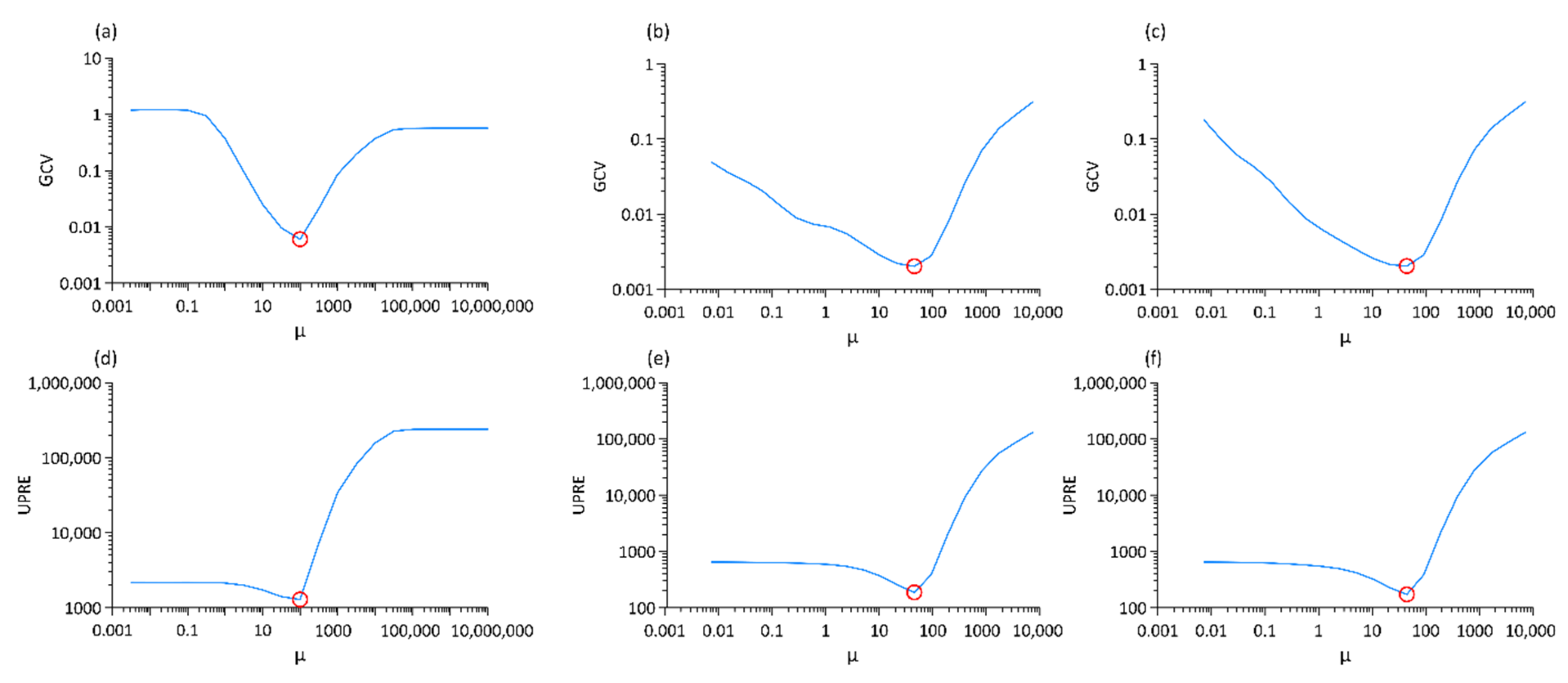
3. Estimation of Regularization Parameter

When estimating the regularization parameter, we only focused on (5) without considering the barrier function. In this way, the regularization parameter is still suitable in the minimization of (7). Here, the GCV [7] and the UPRE [9] methods are used to estimate the regularization parameter.

3.1. Generalized Cross-Validation Method

The randomized trace estimation was introduced into the GCV function to solve the difficulty of a trace calculation in the GCV function [13]. Then, this function for Equation (5) has the form

$$GCV(\mu )\approx \frac{{‖r-h{\left(h^{T}h+{\mu }^2{W}_m{}^T{W}_m\right)}^{-1}{h}^{T}r‖}_2^2}{{\left\{n-R^{T}h{\left(h^{T}h+{\mu }^2{W}_m{}^T{W}_m\right)}^{-1}{h}^{T}R\right\}}^2},$$

(11)

where R is a random vector consisting of −1 and 1, each with a probability of 0.5. The parameter μ which minimizes (11) is the optimal regularization parameter μ_opt. This parameter μ_opt can be determined by line search within a range for regularization parameter, and the process can be solved by using the CG method [13]. However, when using the CG method, an optimal range for regularization parameter is difficult to determine, and sometimes the optimal regularization parameter μ_opt is not within the selected range. Moreover, the GCV method using the CG method is time-consuming.

The GSVD of the matrix pair $\left[h,W_m\right]$ can be used to compute the GCV function [5]. Based on the GSVD, the spectrum of h can be obtained. The optimal linear search range can be determined by analyzing the spectrum of h [9]. However, the calculation of GSVD is time-consuming and has a large memory requirement. When the scale of data is large, the calculation of GSVD is even impractical. Instead, the RGSVD algorithm is adopted. The RGSVD algorithm uses the randomized algorithm to provide a low-rank approximation of the GSVD [10]. Compared with the GSVD, the RGSVD can reduce computational costs and memory demands, and results with good accuracy can be obtained. Algorithm 2 shows the RGSVD algorithm [10], which is used in this study. The parameter q determines the accuracy and efficiency of the RGSVD algorithm. As the value of the parameter q increases, the result becomes more accurate and the computation time is longer.

Algorithm 2. Randomized generalized singular value decomposition (RGSVD) algorithm. $\mathrm{Given} h\in R^{n\times m}$ ($n\le m$) and $W_m\in R^{4m\times m}$, a target matrix rank q ($q\le n$), calculate an approximate GSVD of the matrix pair $\left[h,W_m\right]$$: h\approx UCX$, $W_m\approx VSX$ with $U\in R^{n\times q}$, $V\in R^{4m\times q}$$, C\in R^{q\times q}$, $S\in R^{q\times q}$, and $X\in R^{q\times m}$.

$\mathrm{Generate} \mathrm{a} q\times n$ Gaussian random matrix $A$. Calculate the $q\times m$ matrix $Y=Ah$. Calculate the $m\times q$ orthonormal matrix $Q$ via QR factorization $Y^T=QR$. Form the $n\times q$ matrix $B_1=hQ$ and the $4m\times q$ matrix $B_2=W_{m}Q$. Use $\left[U,V,W,C,S\right]=\mathrm{gsvd}(B_1,B_2,0)$ to calculate the economy-sized GSVD of the matrix pair $\left[B_1,B_2\right]$$: \left[\begin{array}{c}{B}_1\\ B_2\end{array}\right]=\left[\begin{array}{cc}U& \\ & V\end{array}\right]\left[\begin{array}{c}C\\ S\end{array}\right]W^T$. Form the $q\times m$ matrix $X=W^T{Q}^T$. $\mathrm{Note}: h\approx UCX$ and $W_m\approx VSX$.

In the RGSVD algorithm, $C=diag\left(c_1,c_2\dots ,c_q\right)\in R^{q\times q}$ with

$$0<c_1\le c_2\le \cdots \le c_q<1,$$

(12)

and $S=diag\left(s_1,s_2,\dots ,s_2\right)\in R^{q\times q}$ with

$$1>s_1\ge s_2\ge \cdots \ge s_q>0,$$

(13)

$c_i^2+s_i^2=1$, $\forall i=1:q$, that is $C^{T}C+S^{T}S=I_q$. According to the result of the RGSVD, Equation (11) has the form

$$GCV(\mu )\approx \frac{{‖r-h\left[{\displaystyle \sum _{i=1}^q\frac{{\gamma }_i^2}{{\gamma }_i^2+{\mu }^2}\frac{u_i^{T}r}{c_i}{(X^{†})}_i}\right]‖}_2^2}{{\left\{n-R^{T}h\left[{\displaystyle \sum _{i=1}^q\frac{{\gamma }_i^2}{{\gamma }_i^2+{\mu }^2}\frac{u_i^{T}R}{c_i}{(X^{†})}_i}\right]\right\}}^2},$$

(14)

where ${\gamma }_i={c_i/s}_i$ denotes the ith generalized singular value, $u_i$ represents the ith column of matrix U, and ${(X^{†})}_i$ denotes the ith column of the Moore-Penrose inverse of matrix X. The parameter μ_opt can be found between the minimum and maximum of the generalized singular value ${\gamma }_i$. Here, the parameter q is set as n. Therefore, the full generalized singular values can be obtained. The value of n is slightly large, but the computation time of the RGSVD algorithm with $q=n$ is still much shorter than that of GSVD.

3.2. Unbiased Predictive Risk Estimator Method

The UPRE function for Equation (5) has the form [16]

$$\begin{array}{l}UPRE(\mu )={‖r-h{\left(h^{T}h+{\mu }^2{W}_m{}^T{W}_m\right)}^{-1}{h}^{T}r‖}_2^2\\ +2 trace\left[h{\left(h^{T}h+{\mu }^2{W}_m{}^T{W}_m\right)}^{-1}{h}^T\right]-n\end{array},$$

(15)

where $trace\left[ \right]$ is the trace of the term in the brackets. The randomized trace estimation [9] was also introduced in Equation (15) to solve the difficulty from the calculation of the trace. Then, the UPRE function is approximated by

$$\begin{array}{l}UPRE(\mu )\approx {‖r-h{\left(h^{T}h+{\mu }^2{W}_m{}^T{W}_m\right)}^{-1}{h}^{T}r‖}_2^2\\ +2 R{ }^T h{\left(h^{T}h+{\mu }^2{W}_m{}^T{W}_m\right)}^{-1}{h}^{T}R-n\end{array}.$$

(16)

The result of the RGSVD is introduced into Equation (16), and Equation (16) has the form

$$\begin{array}{l}UPRE(\mu )\approx {‖r-h\left[{\displaystyle \sum _{i=1}^q\frac{{\gamma }_i^2}{{\gamma }_i^2+{\mu }^2}\frac{u_i^{T}r}{c_i}{(X^{†})}_i}\right]‖}_2^2\\ +2 R^{T}h\left[{\displaystyle \sum _{i=1}^q\frac{{\gamma }_i^2}{{\gamma }_i^2+{\mu }^2}\frac{u_i^{T}R}{c_i}{(X^{†})}_i}\right]-n\end{array}.$$

(17)

Similarly, when the value of Equation (17) is the minimum, its corresponding parameter μ is the optimal regularization parameter μ_opt, which can be found between the minimum and maximum of the generalized singular value ${\gamma }_i$ as well. Here, the parameter q is also set as n.

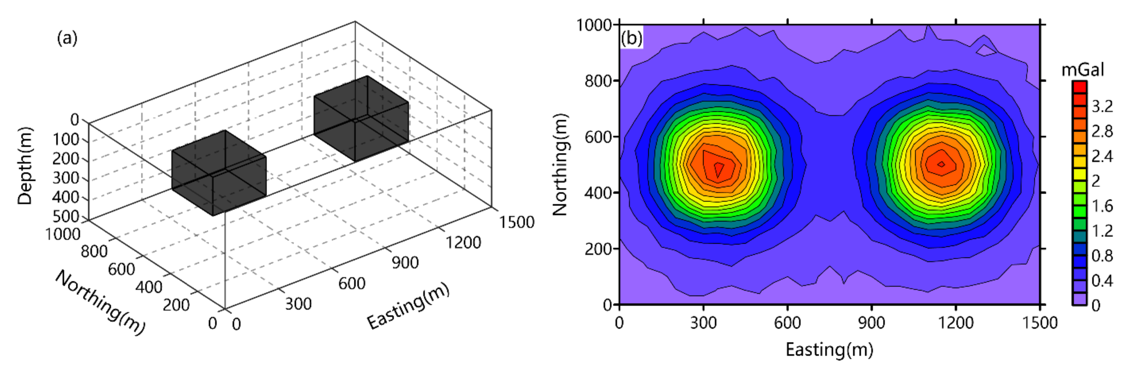
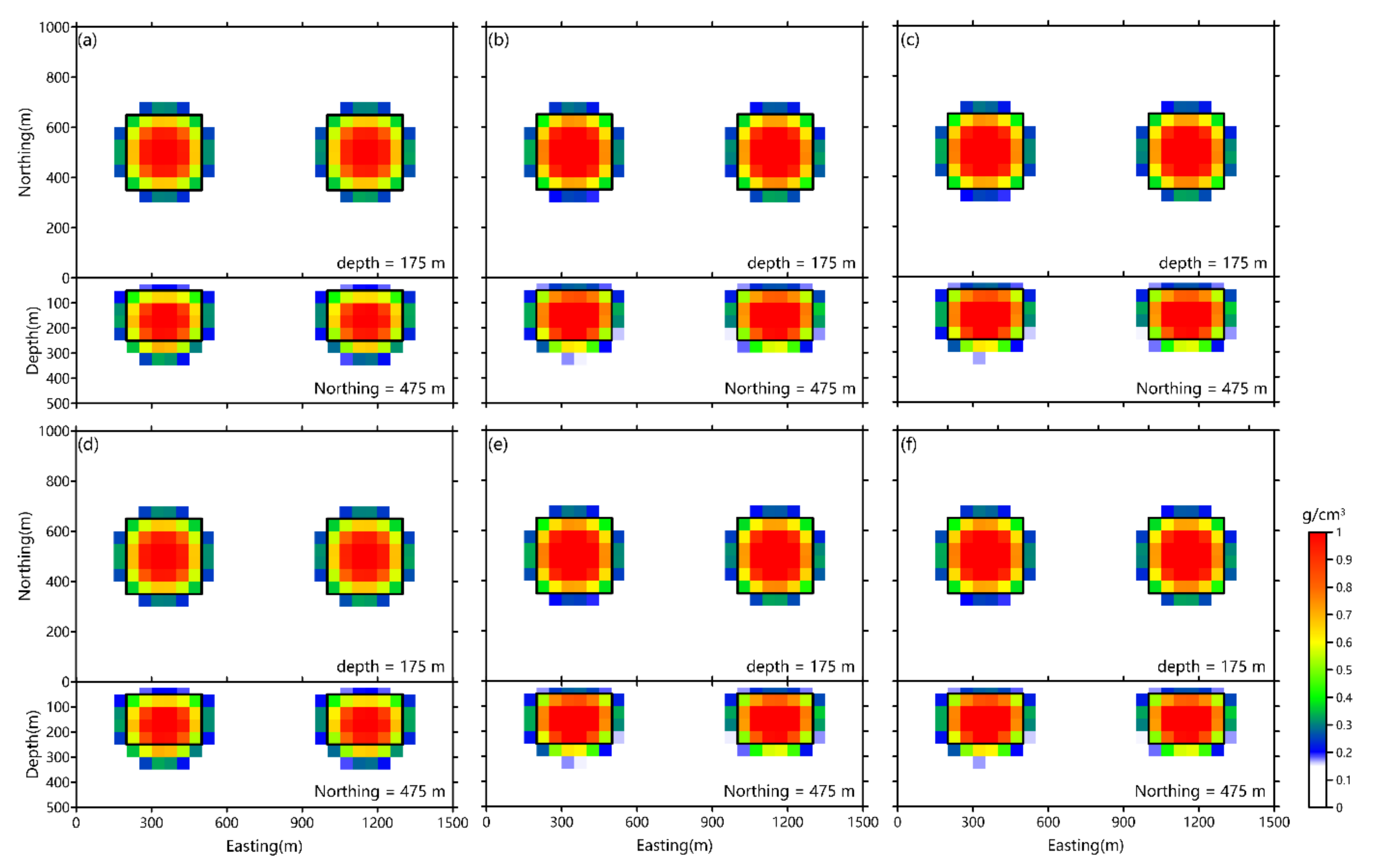
4. Synthetic Example Tests

In this study, one example was used to demonstrate the performances of the GCV and the UPRE methods using the RGSVD algorithm. For comparison, the CG method and the GSVD method were also used in the GCV and UPRE methods. The following tests were run on a computer with a 3.00 GHz processor and 32 GB RAM.

The model consists of two cuboids, and Figure 1a shows its 3D perspective view. The dimensions of the two cuboids are both 300 m × 300 m × 200 m, and the depths of their tops are both 50 m. Both of them have a density contrast of 1 g/cm³. The gravity data were generated on a grid with 31 × 21 = 651 points and 50 m × 50 m spacings. Meanwhile, random Gaussian noise, whose standard deviation is 0.02 mGal plus 2% of each datum, were incorporated in the gravity data (Figure 1b). The subsurface was divided into 30 × 20 × 10 = 6000 cells, and dimension of each cell is 50 m × 50 m × 50 m. In the following inversions, the density range was 0–1 g/cm³ and $K_{\max }$ was set as 50.

First, we used the GCV method to determine the regularization parameter in inversion. In the GCV method, the CG method, the GSVD, and the RGSVD algorithm were used, respectively. Figure 2a–c show the inversion results from the GCV methods using the CG method, the GSVD, and the RGSVD algorithm, respectively. These three inversion results are very similar: two source bodies with cuboid shape are in the actual position of the true model. Their corresponding GCV function curves are shown in Figure 3a–c, and these three curves have similar trends. Meanwhile,

Table 1. The optimal regularization parameters and the elapsed times for different regularization methods.

	GCV Method			UPRE Method
	CG	GSVD	RGSVD	CG	GSVD	RGSVD
${\mu }_{opt}$	100.0	45.3	44.4	100.0	45.3	44.4
Time	117.5 s	113.0 s	1.3 s	111.2 s	114.3 s	1.4 s

Note: μ_opt is the optimal regularization parameter, and Time denotes the elapsed time for different regularization method.

records the corresponding optimal regularization parameters μ_opt, and the corresponding elapsed times for the process of choosing the regularization parameter. The GCV methods using the GSVD and the RGSVD algorithm have very similar μ_opt, and the μ_opt of the GCV method using the CG method is slightly large. The GCV method using the RGSVD algorithm has the shortest elapsed time, at only 1.3 s.

Then, the UPRE method was implemented in inversion. Similarly, the UPRE method used the CG method, GSVD, and the RGSVD algorithm, respectively. Their inversion results are shown in Figure 2d–f, respectively. These inversion results are similar to those obtained using the GCV method. The curves for the UPRE function are demonstrated in Figure 3d–f, and they also have similar trends. Table 1 also lists the value of optimal regularization parameters and the elapsed times for the UPRE method. Their optimal regularization parameters are the same as them from the GCV method, and the elapsed times are close to them from the GCV method. The UPRE method using the RGSVD algorithm also has the shortest elapsed time.

Through the above comparative test, it was concluded that the GCV and the UPRE methods using the RGSVD algorithm can quickly provide an optimal regularization parameter that can generate a satisfying inversion result.

5. Conclusions

We introduced the GCV and the UPRE methods using the RGSVD algorithm, with which the optimal regularization parameter can be determined fast in the inversion of potential field data. We demonstrated the effect of these two methods through a comparative test.

References

1. Yan, J.; Lü, Q.; Chen, X.; Qi, G.; Liu, Y.; Guo, D.; Chen, Y. 3D lithologic mapping test based on 3D inversion of gravity and magnetic data: A case study in Lu-Zong ore concentration district, Anhui Province. Acta Petrol. Sin. 2014, 30, 1041–1053. [Google Scholar]
2. Yan, J.; Chen, X.; Meng, G.; Lü, Q.; Deng, Z.; Qi, G.; Tang, H. Concealed faults and intrusions identification based on multi-scale edge detection and 3D inversion of gravity and magnetic data: A case study in Qiongheba area, Xinjiang, Northwest China. Interpretation 2019, 7, T331–T345. [Google Scholar] [CrossRef]
3. Wang, J.; Meng, X.; Li, F. Fast Nonlinear Generalized Inversion of Gravity Data with Application to the Three-Dimensional Crustal Density Structure of Sichuan Basin, Southwest China. Pure Appl. Geophys. 2017, 174, 4101–4117. [Google Scholar] [CrossRef]
4. Tikhonov, A.N.; Arsenin, V.Y. Solutions of Ill-Posed Problems. Math. Comput. 1977, 32, 491. [Google Scholar]
5. Vatankhah, S.; Ardestani, V.E.; Renaut, R.A. Automatic estimation of the regularization parameter in 2D focusing gravity inversion: Application of the method to the Safo manganese mine in the northwast of Iran. J. Geophys. Eng. 2014, 11, 045001. [Google Scholar] [CrossRef] [Green Version]
6. Morozov, V.A. On the solution of functional equations by the method of regularization. Sov. Math. Dokl. 1966, 7, 414–417. [Google Scholar]
7. Golub, G.H.; Heath, M.; Wahba, G. Generalized cross-validation as a method for choosing a good ridge regression parameter. Technometrics 1979, 21, 215–223. [Google Scholar] [CrossRef]
8. Hansen, P.C. Analysis of discrete ill-posed problems by means of the L-curve. SIAM Rev. 1992, 34, 561–580. [Google Scholar] [CrossRef]
9. Vogel, C.R. Computational Methods for Inverse Problems. In SIAM Frontiers in Applied Mathematics; SIAM: Philadelphia, PA, USA, 2002. [Google Scholar]
10. Wei, Y.; Xie, P.; Zhang, L. Tikhonov Regularization and Randomized GSVD. SIAM J. Matrix Anal. Appl. 2016, 37, 649–675. [Google Scholar] [CrossRef]
11. Li, Y.; Oldenburg, D.W. 3-D inversion of magnetic data. Geophysics 1996, 61, 394–408. [Google Scholar] [CrossRef]
12. Li, Y.; Oldenburg, D.W. 3-D inversion of gravity data. Geophysics 1998, 63, 109–119. [Google Scholar] [CrossRef]
13. Li, Y.; Oldenburg, D.W. Fast inversion of large-scale magnetic data using wavelet transforms and a logarithmic barrier method. Geophys. J. Int. 2003, 152, 251–265. [Google Scholar] [CrossRef] [Green Version]
14. Li, Z.; Yao, C.; Zheng, Y.; Wang, J.; Zhang, Y. 3D magnetic sparse inversion using an interior-point method. Geophysics 2018, 83, J15–J32. [Google Scholar] [CrossRef]
15. Li, Z.; Yao, C. 3D sparse inversion of magnetic amplitude data when strong remanence exists. Acta Geophys. 2020, 68, 365–375. [Google Scholar] [CrossRef]
16. Vatankhah, S.; Renaut, R.A.; Ardestani, V.E. Total variation regularization of the 3-D gravity inverse problem using a randomized generalized singular value decomposition. Geophys. J. Int. 2018, 213, 695–705. [Google Scholar] [CrossRef] [Green Version]
Figure 1. (a) 3D perspective view of the model consisting of two cuboids; (b) gravity data produced by this model.
Applsci 11 06326 g001
Figure 2. Inversion results from different regularization methods. The generalized cross-validation (GCV) methods using (a) the conjugate gradient (CG) method, (b) the generalized singular value decomposition (GSVD), and (c) the randomized generalized singular value decomposition (RGSVD algorithm; the unbiased predictive risk estimator (UPRE) methods using (d) the CG method, (e) the GSVD, and (f) the RGSVD algorithm. In all these panels, the black lines indicate the real position of the model.
Applsci 11 06326 g002
Figure 3. The GCV functions using (a) the CG method, (b) the GSVD, and (c) the RGSVD algorithm; the UPRE functions using (d) the CG method, (e) the GSVD, and (f) the RGSVD algorithm. The blue curve is GCV function or UPRE function, and the red ○ is the optimal regularization parameter.
Applsci 11 06326 g003