
Study on Two-Phase Mixing Inside Flow Focusing/Blurring Nozzle by Gray Distribution Analysis Method

Abstract
:1. Introduction
2. Materials and Methods
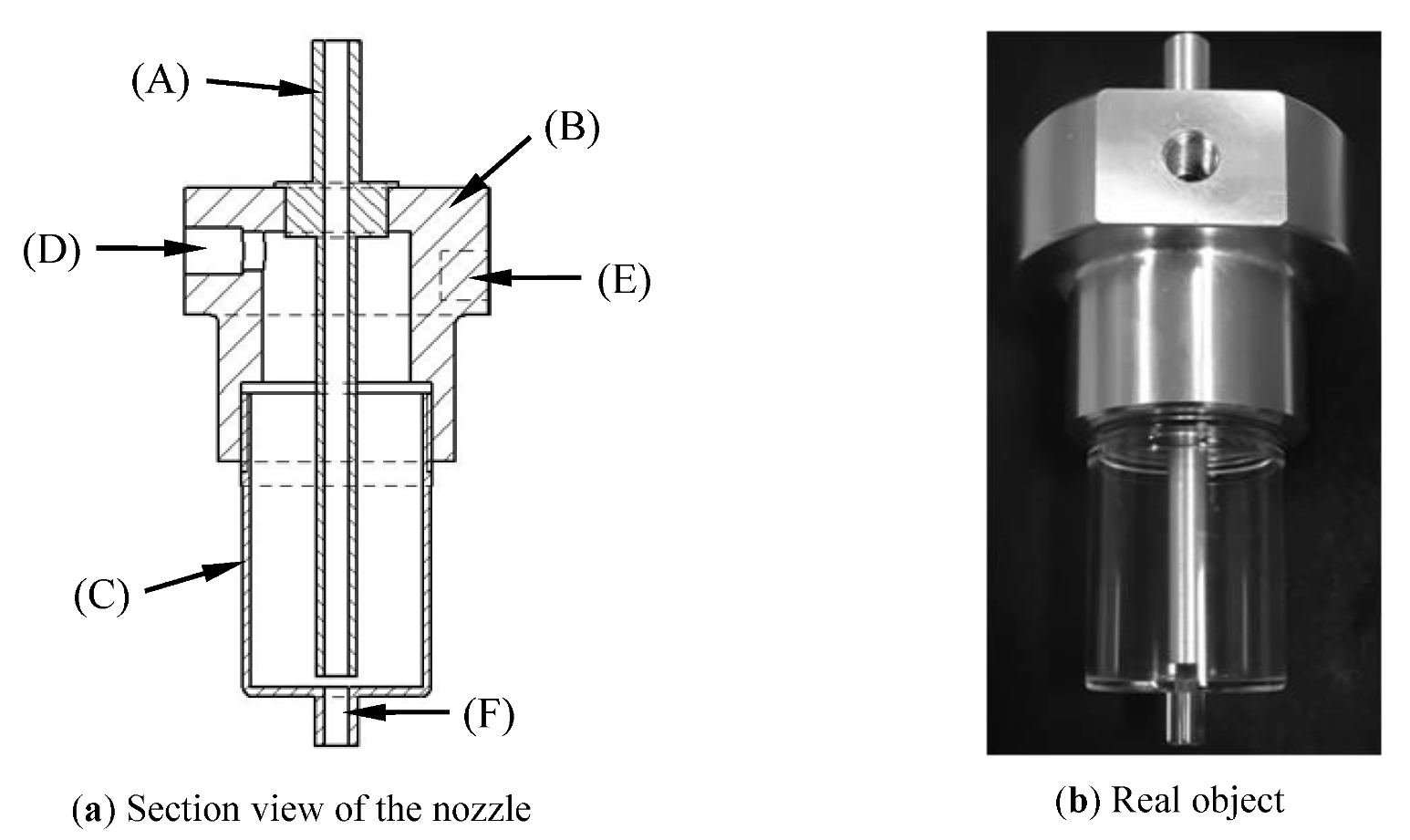
2.1. Atomizer
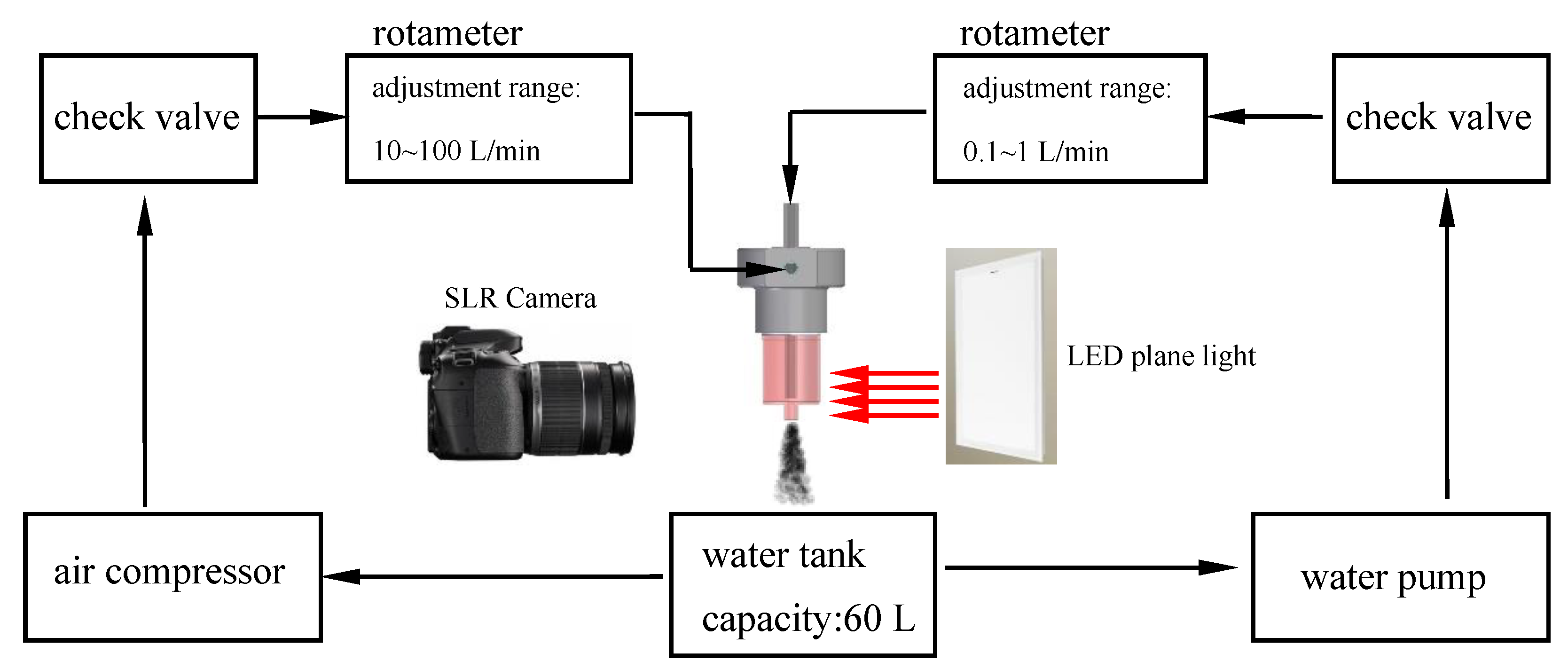
2.2. Experimental Platform
3. Gray Distribution Analysis of Experimental Images
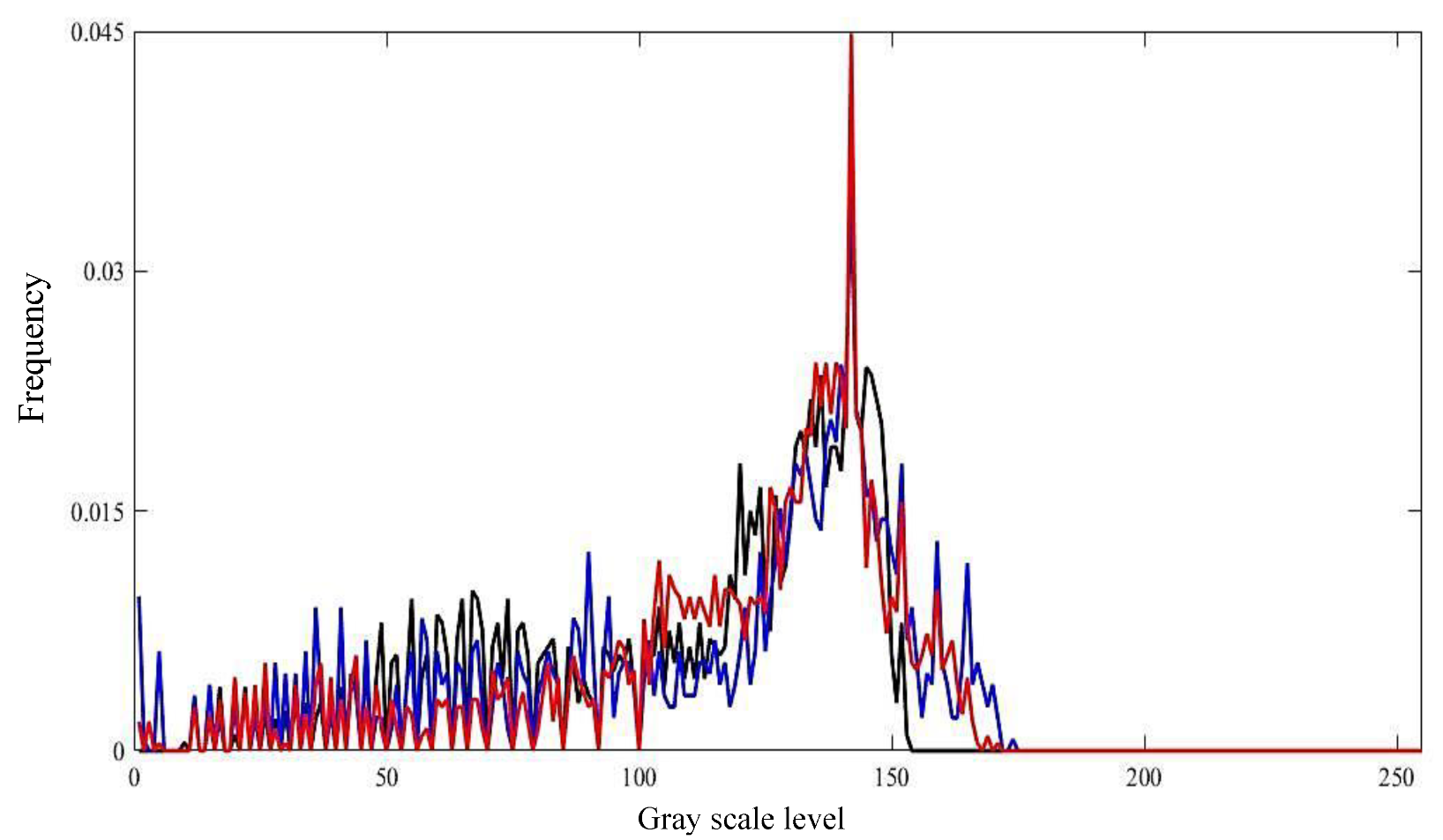
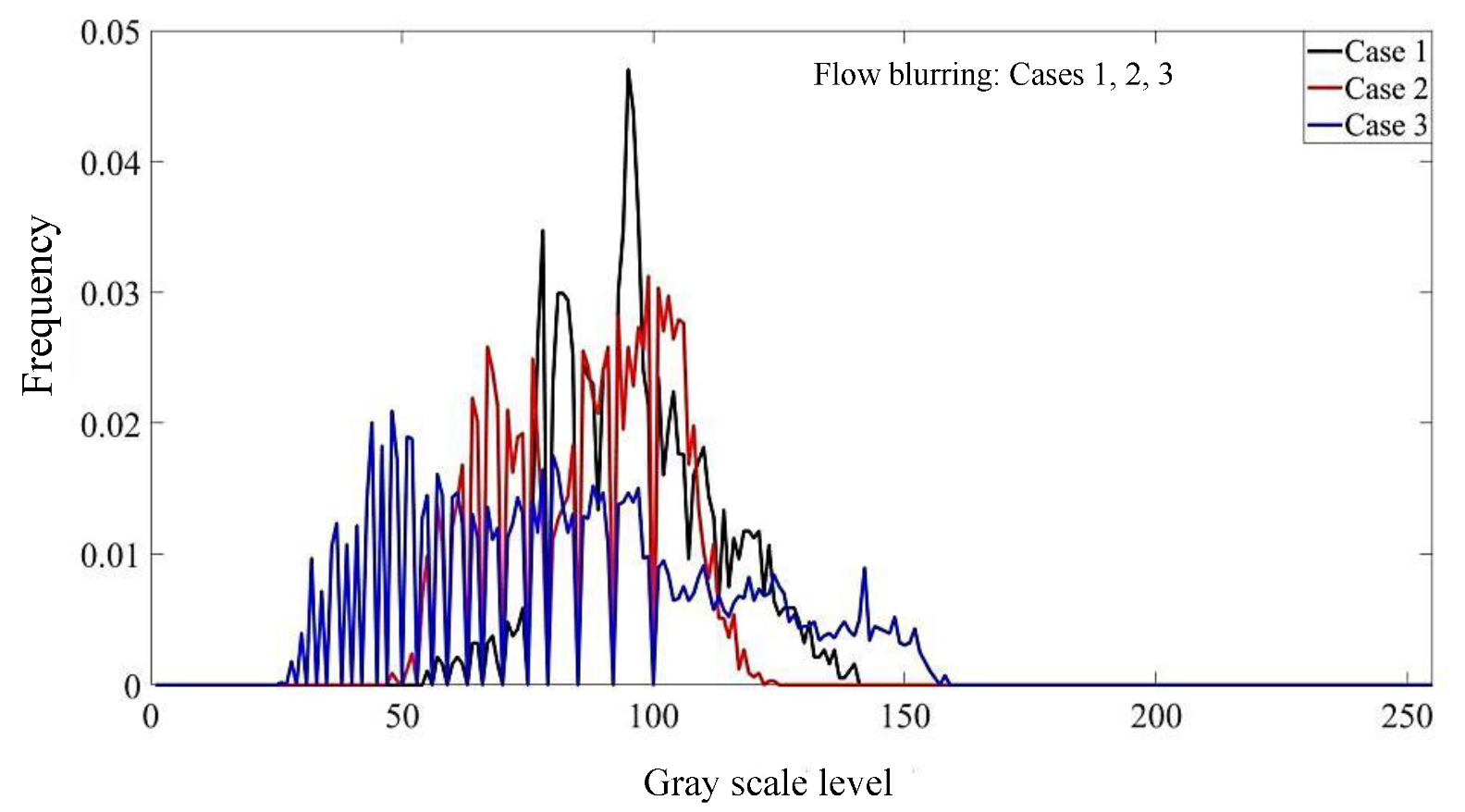
3.1. Gray Distribution of Image
3.2. Feasibility Analysis
4. Results and Discussions
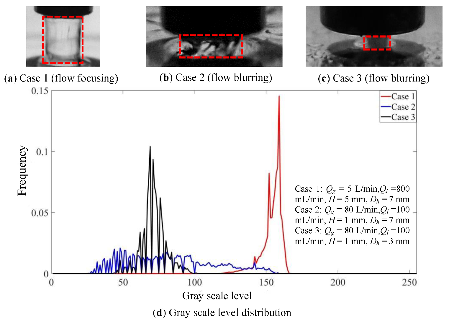
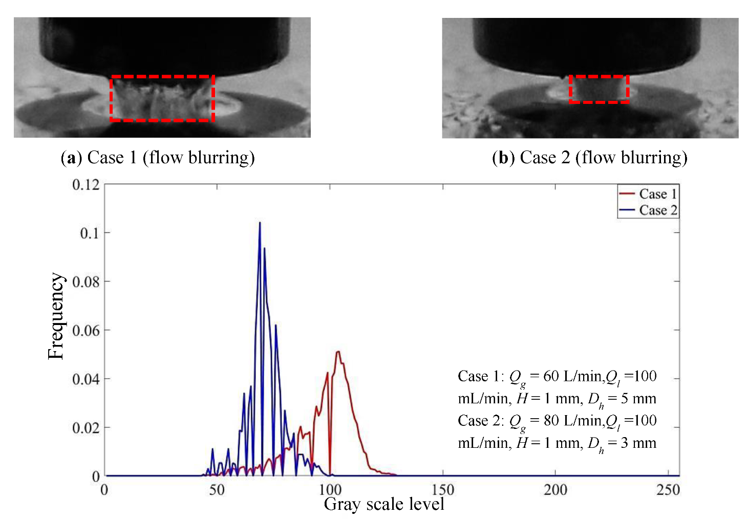
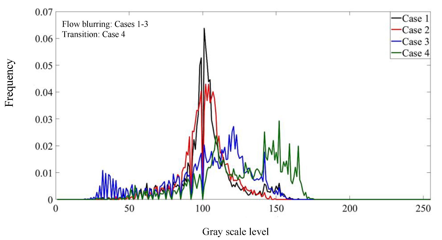
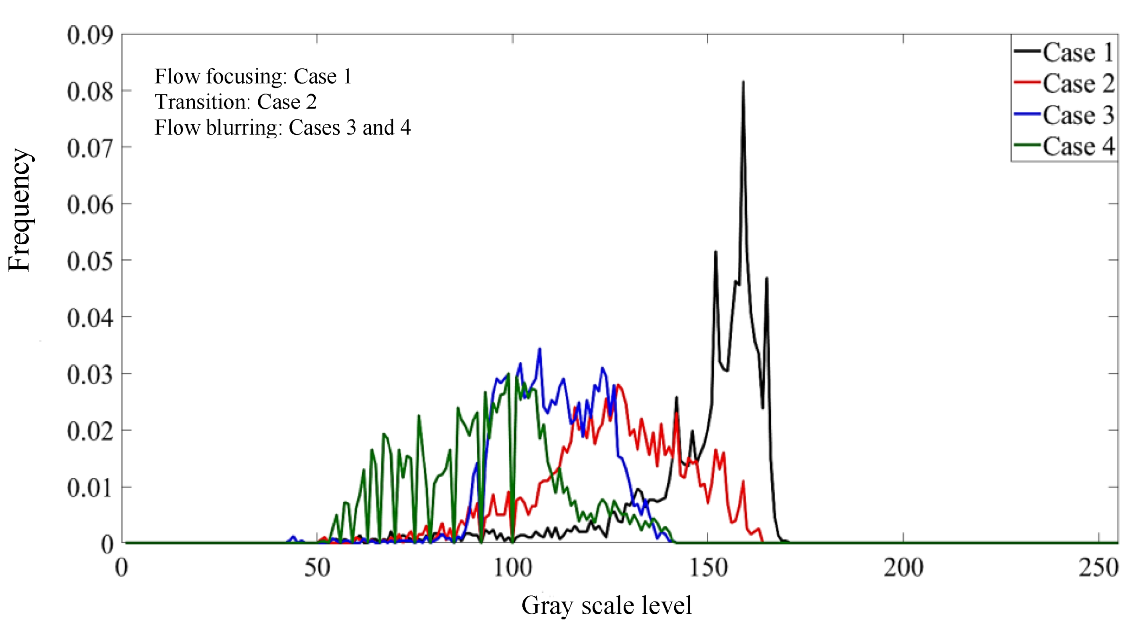
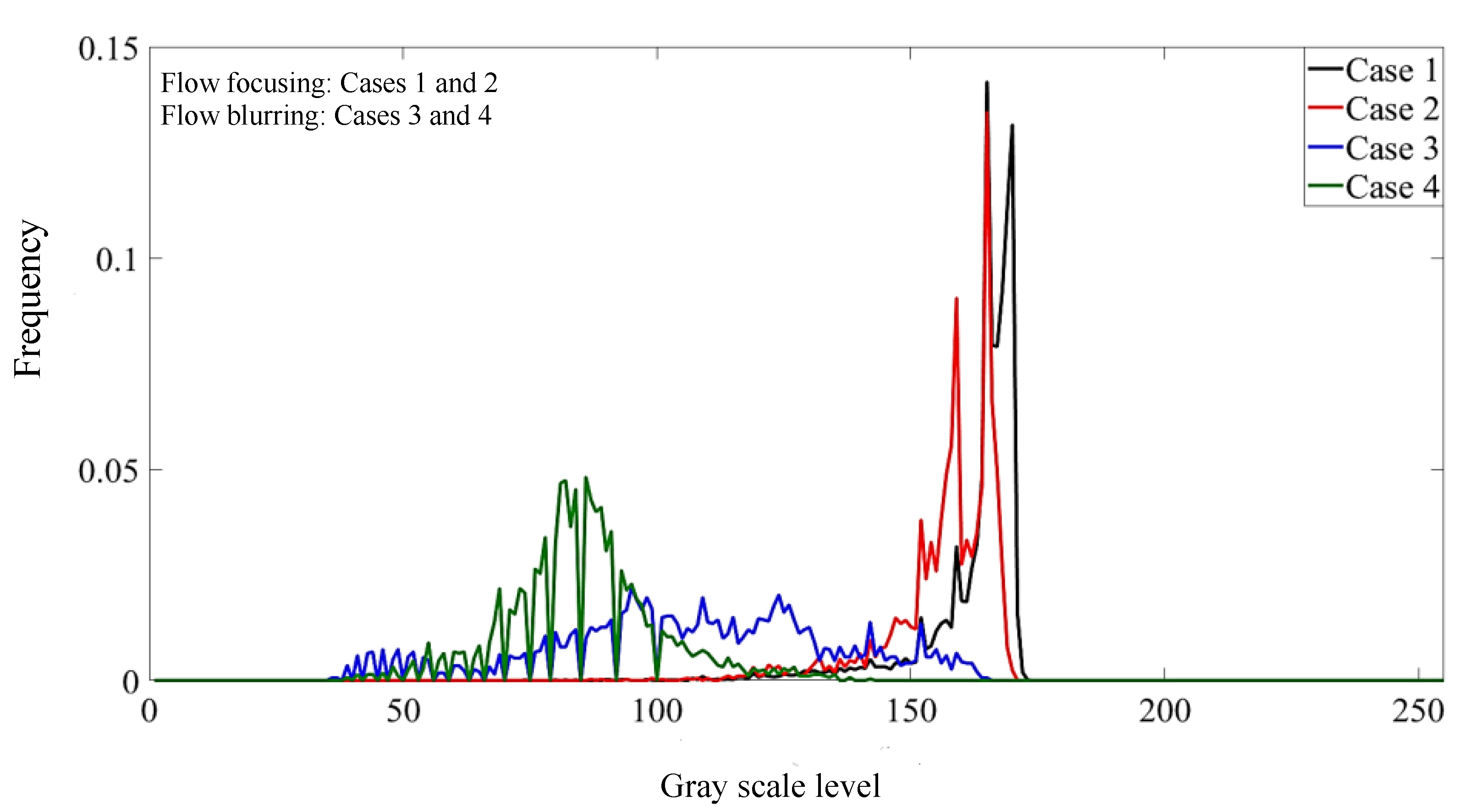
4.1. The Influence of Flow and Structure Parameters on Two-Phase Mixing Inside the Nozzle
4.2. Comparison of the Influence of Different Parameters on Two-Phase Mixing
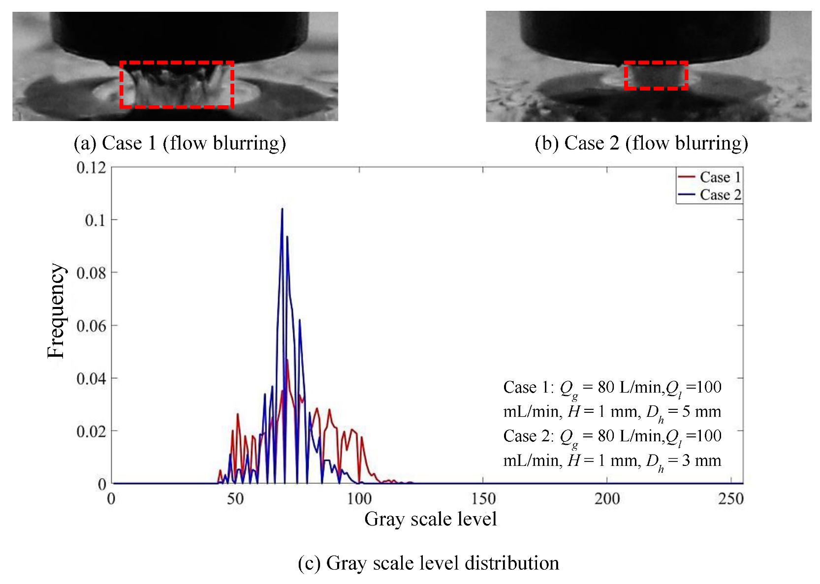
4.3. Local Analysis of Two-Phase Flow Field in Mixing Zone
5. Conclusions
Author Contributions
Funding
Institutional Review Board Statement
Informed Consent Statement
Data Availability Statement
Conflicts of Interest
References
- Ganan-Calvo, A.M. Generation of steady liquid microthreads and micron-sized monodisperse sprays in gas streams. Phys. Rev. Lett. 1998, 80, 285–288. [Google Scholar] [CrossRef]
- Ganan-Calvo, A.M. Enhanced liquid atomization: From flow-focusing to flow-blurring. Appl. Phys. Lett. 2005, 86, 4601. [Google Scholar] [CrossRef]
- Si, T.; Yin, X.Z. Progress and application of flow focusing. Chin. Sci. Bull. 2011, 56, 537–546. [Google Scholar] [CrossRef]
- Ganan-Calvo, A.M.; González-Prieto, R.; Riesco-Chueca, P.; Herrada, M.A.; Flores-Mosquera, M. Focusing Capillary Jets Close to the Continuum Limit. Nat. Phys. 2007, 3, 737–742. [Google Scholar] [CrossRef]
- Vega, E.J.; Montanero, J.M.; Herrada, M.A.; Ganan-Calvo, A. Global and local instability of flow focusing: The influence of the geometry. Phys. Fluids 2010, 22, 064105. [Google Scholar] [CrossRef]
- Montanero, J.M.; Muñoz, N.R.; Herrada, M.A.; Ganan-Calvo, A. Global stability of the focusing effect of fluid jet flows. Phys. Rev. E 2011, 83, 036309. [Google Scholar] [CrossRef] [PubMed]
- Herrada, M.A.; Ganan-Calvo, A.; Ojeda-Monge, A.; Bluth, B.; Riesco-Chueca, P. Liquid flow focused by a gas: Jetting, dripping, and recirculation. Phys. Rev. E 2008, 78, 036323. [Google Scholar] [CrossRef] [PubMed] [Green Version]
- Si, T.; Li, F.; Yin, X.-Y. Modes in flow focusing and instability of coaxial liquid–gas jets. J. Fluid Mech. 2009, 629, 1–23. [Google Scholar] [CrossRef] [Green Version]
- Jiang, L.; Agrawal, A.K. Investigation of Glycerol Atomization in the Near-Field of a Flow-Blurring Injector using Time-Resolved PIV and High-Speed Visualization. Flow Turbul. Combust. 2015, 94, 323–338. [Google Scholar] [CrossRef]
- Jiang, L.L. Investigation of Atomization Mechanisms and Flame Structure of a Twin-Fluid Injector for Different Liquid Fuels. Ph.D. Thesis, The University of Alabama, Tuscaloosa, AL, USA, 2014. [Google Scholar]
- Simmons, B.M.; Agrawal, A.K. Flow Blurring Atomization for Low-Emission Combustion of Liquid Biofuels. Combust. Sci. Technol. 2012, 184, 660–675. [Google Scholar] [CrossRef]
- De Azevedo, C.G.; Andrade, J.C.D.; Costa, F.D.S. Characterization of a blurry injector for burning biofuels in a compact flameless combustion chamber. In Proceedings of the 14th Brazilian Congress of Thermal Sciences and Engineering, Rio de Janeiro, Brazil, 18–22 November 2012. [Google Scholar]
- Xiao, Q.-T.; Pan, J.-X.; Xu, J.-X.; Wang, H.; Lv, Z.-H. Hypothesis-testing combined with image analysis to quantify evolution of bubble swarms in a direct-contact boiling heat transfer process. Appl. Therm. Eng. 2017, 113, 851–857. [Google Scholar] [CrossRef]
- Xiao, Q.; Yang, K.; Wu, M.; Pan, J.; Xu, J.; Wang, H. Complexity evolution quantification of bubble pattern in a gas-liquid mixing system for direct-contact heat transfer. Appl. Therm. Eng. 2018, 138, 832–839. [Google Scholar] [CrossRef]
- Xiao, Q.; Luo, W.; Huang, J.; Xu, J.; Wang, H. Interplay of fluids mixing and heat transfer in a dual-loop ORC direct contact heat exchanger used for waste heat utilization. Inst. Mech. Eng. Part C J. Mech. Eng. Sci. 2020, 234, 2294–2305. [Google Scholar] [CrossRef]
- Wang, C.; Yang, P.Y.; Xu, J.X.; Wang, S.B.; Wang, H. Study on flow regime identification of gas-liquid two phase flows in the mixing process by top blowing. J. Kunming Univ. Sci. Technol. 2014, 39, 77–82. [Google Scholar]
- Yang, L. Study of Gray Feature of Water Bubbles Group Image. Master’s Thesis, Harbin Engineering University, Harbin, China, 2015. [Google Scholar]
- Li, X.; Liu, N.; Hao, P.; Zhang, X.; He, F. Screech feedback loop and mode staging process of axisymmetric underexpanded jets. Exp. Therm. Fluid Sci. 2021, 122, 110323. [Google Scholar] [CrossRef]
- Li, X.-R.; Zhang, X.-W.; Hao, P.-F.; He, F. Acoustic feedback loops for screech tones of underexpanded free round jets at different modes. J. Fluid Mech. 2020, 902. [Google Scholar] [CrossRef]
- Semlitsch, B.; Malla, B.; Gutmark, E.J.; Mihăescu, M. The generation mechanism of higher screech tone harmonics in supersonic jets. J. Fluid Mech. 2020, 893. [Google Scholar] [CrossRef] [Green Version]
- Gonzalez, R.C.; Woods, R.E. Digital Image Processing, 4th ed.; Pearson: London, UK, 2017. [Google Scholar]


| Parameter | Symbol | Value/mm |
|---|---|---|
| Nozzle inner tube diameter | D | 5 |
| Tube hole distance | H | 1/2/3/4/5 |
| Orifice diameter | Dh | 3/5/7 |
| Hole length | lh | 10 |
Publisher’s Note: MDPI stays neutral with regard to jurisdictional claims in published maps and institutional affiliations. |
© 2021 by the authors. Licensee MDPI, Basel, Switzerland. This article is an open access article distributed under the terms and conditions of the Creative Commons Attribution (CC BY) license (https://creativecommons.org/licenses/by/4.0/).
Share and Cite
Zhao, J.; Ning, Z.; Lü, M.; Sun, C. Study on Two-Phase Mixing Inside Flow Focusing/Blurring Nozzle by Gray Distribution Analysis Method. Appl. Sci. 2021, 11, 6260. https://doi.org/10.3390/app11146260
Zhao J, Ning Z, Lü M, Sun C. Study on Two-Phase Mixing Inside Flow Focusing/Blurring Nozzle by Gray Distribution Analysis Method. Applied Sciences. 2021; 11(14):6260. https://doi.org/10.3390/app11146260
Chicago/Turabian StyleZhao, Jin, Zhi Ning, Ming Lü, and Chunhua Sun. 2021. "Study on Two-Phase Mixing Inside Flow Focusing/Blurring Nozzle by Gray Distribution Analysis Method" Applied Sciences 11, no. 14: 6260. https://doi.org/10.3390/app11146260
APA StyleZhao, J., Ning, Z., Lü, M., & Sun, C. (2021). Study on Two-Phase Mixing Inside Flow Focusing/Blurring Nozzle by Gray Distribution Analysis Method. Applied Sciences, 11(14), 6260. https://doi.org/10.3390/app11146260