Article

Application Study on Fiber Optic Monitoring and Identification of CRTS-II-Slab Ballastless Track Debonding on Viaduct

1
School of Civil Engineering, Wuhan University, Wuhan 430072, China
2
Key Laboratory for Resilient Infrastructures of Coastal Cities (MOE), College of Civil and Transportation Engineering, Shenzhen University, Shenzhen 518060, China
3
School of Computer Science and Engineering, Beihang University, Beijing 100191, China
4
Structural Health Monitoring and Control Institute, Shijiazhuang Tiedao University, Shijiazhuang 050043, China
*
Authors to whom correspondence should be addressed.
Appl. Sci. 2021, 11(13), 6239; https://doi.org/10.3390/app11136239
Submission received: 13 May 2021 / Revised: 22 June 2021 / Accepted: 3 July 2021 / Published: 5 July 2021

Abstract

:
China Railway Track System (CRTS)-II-slab ballastless track is a new type of track structure, and its interlayer connection state is considerably important for the operation safety and ride comfort of high-speed trains. However, the location and multiple influencing factors of interlayer debonding lead to difficulties in monitoring and identification. Here, the research on the design and application of a monitoring scheme that facilitates interlayer debonding detection of ballastless track and an effective indicator for debonding identification and assessment is proposed. The results show that on-site monitoring can effectively capture the vibration signals caused by train vibration and interlayer debonding. The features of the data acquired in the situations with and without interlayer debonding are compared after instantaneous baseline validation. Some significant features capable of obviously differentiating a debonding state from the normal state are identified. Furthermore, a new indicator, combining multiple debonding-sensitive features by similarity-based weights normalizing the initial difference between mutual instantaneous baselines, is developed to support rational and comprehensive assessment quantitatively. The contribution of this study includes the development and application of an interlay-debonding monitoring scheme, the establishment of an effective-feature pool, and the proposal of the similarity-based indicator, thereby laying a good foundation for debonding identification of ballastless track.

1. Introduction

The CRTS-II-slab ballastless track in the China high-speed railway (HSR) track system is a new type of track structure that is developed on the basis of Germany’s Burger-slab ballastless track system. The foundation of the CRTS-II-slab ballastless track in China takes the forms of viaducts or subgrades, of which viaducts account for a large proportion of the rail line. For example, the viaducts of Beijing–Tianjin intercity railway and Beijing–Shanghai HSR account for 93% and 91.8% of the whole line, respectively [1]. The CRTS-II-slab ballastless track on the viaduct consists of rail, track slab, cement emulsified asphalt mortar (CA mortar) layer, concrete supporting layer, and bridge deck. The track slab and the concrete supporting layer are connected by a cast-in-place CA mortar layer, and the concrete supporting layer and the bridge deck are connected by a so-called “two cloth and one film sliding layer”, forming a monolithic layering structure vertically. The adjacent track slabs are connected by cast-in-place joints in the longitudinal direction, constituting a seamless structure. This type of track structure is widely advocated for its low vibration and noise, good smoothness, and lower maintenance. Nonetheless, during the long-term service life, the track structure may suffer from various problems, such as cracking of track slab, debonding between track slab and CA mortar layer, and slab upwarping [2,3,4,5]. Under the double effects of operational and environmental loads, the debonding between track slab and CA mortar layer tends to develop into a void of CA mortar layer and slab upwarping. Interlayer debonding is the root cause of the void defect of CA mortar layer and upwarping defect of the track slab, so it has attracted the focused attention of scholars and engineers, and it is also the focus of this study.
Investigations into nondestructive testing (NDT) and structural health monitoring (SHM) of ballastless rail track and concrete slabs are globally existent and extensive. A group of scholars from Taiwan and Hong Kong studied the detection of delaminated cracks inside the CA mortar layer by a nondestructive method and validated the method by using a sandwiched slab specimen [6]. They used amplitude spectra of impact–echo (IE) waveform to detect the delaminated flaw inside the CA mortar layer of the HSR track, and the results showed that the method could identify different lateral sizes of cracks in the CA mortar layer of a concrete–CA mortar–concrete sandwiched slab specimen. Hoda et al. in the United States investigated the assessing sensitivity of impact–echo and ultrasonic-surface-wave (USW) methods for nondestructive evaluation of concrete structures [7]. They employed the dominant frequency of the IE waveform, and the USW dispersion curves to identify the artificial defects (delaminated zones, air void, or water void) embedded in the center of the slabs at different depths. Taekeun et al. in Korea applied three different processing methods for analyzing data acquired from the IE test of a concrete slab with simulated delamination and void defects, namely the classical impact–echo method, the peak frequency map, and the 4D spectrum technique [8]. In addition, several other approaches, including hammer test [9,10], full-wavefield imaging [11], and ground-penetrating radar (GPR) [12,13,14] methods, have been employed by scholars in different countries for the damage detection of the track or concrete slab. Guidelines for track maintenance are commonly seen in both eastern and western areas [15,16]. Regarding the NDT of CRTS-II-slab ballastless track for debonding detection, Yin [17] employed on-board sensors on a vehicle, and Yang et al. [14] used a GPR method to detect debonding. Tian et al. [18] adopted the IE method and took advantage of elastic waves to identify interlayer defects. Some of the investigations, including the NDT using IE [18] and GPR [14] methods, belong to the partners/colleagues of the authors in this paper, and their experiments were conducted on a CRTS-II-slab track model with mortar defects. The NDT techniques are generally performed intermittently by technical personnel or inspection vehicle going to the field for examining specific sections of track, leading to the late awareness of damage and the occupation of skylight time or the interruption of the normal operation of the high-speed train.
Structural health monitoring, supporting timely detection of damage, and exempting the interruption of the normal operation of a monitored system (e.g., track-vehicle system), has been widely applied to different civil structures [19,20,21,22,23,24,25,26,27,28,29,30,31,32,33,34,35,36,37]. Examples in railway engineering without the interruption of the normal operation of the train include the interval dynamic analysis of the train–bridge system [23], rail crack identification [24], wheel damage detection [21,25], and track condition monitoring [26,27,28,29,30,31,32,33,34,35,36,37]. The studies on track condition monitoring involve track slab deformation measurement by using computer vision [33,34], dynamic strain and acceleration [27], and displacement measurement [28] by remote sensing, measurement of different parameters (such as stress and sound wave) by using wireless sensor networks [29], deformation measurement by using fiber Bragg grating (FBG) sensors [30,31,32,33], or distributed fiber optic sensors [34,35], track axial force measurement by using FBG sensors and electronic sensors [36], and geometrical rail track condition monitoring by using FBG and Raman distributed temperature sensors [37]. Both fiber optic sensors and piezoelectric sensors are commonly used in SHM. As the voltage of HSR can reach thousands or even tens of thousands of volts, traditional piezoelectric vibration sensors are potentially subjected to great electromagnetic interference. Fiber optic sensing technology [38] takes light waves as a carrier and fiber as a medium, which has the advantages of anti-electromagnetic interference, corrosion resistance, long-distance transmissibility, strong multiplexing, and networking ability, and thus meeting the needs of on-site monitoring of rail track. The partners of the authors in this paper have developed interferometric fiber optic accelerometers for vibration measurement [39]. These sensors were used for measuring the vibration of a CRTS-II-slab track and investigating the relationship between temperature and track vibration [40]. Different from the previous investigations, a monitoring scheme that facilitates interlayer debonding detection of in-service CRTS II slab track and diminishes the influence of environmental and operational conditions on feature and indicator comparison is developed in this study. Fiber optic vibration sensors [39] are deployed in a cable trough because in the region allowed for sensor placement, the cable trough is the transversely nearest place to the debonding-prone area. Conventionally, feature comparison between the situations with and without damage is based on the comparison of the current feature to a pre-stored baseline built when the structure was in its pristine state. This comparison between current data and past pristine baseline data (i.e., the subtraction between them) can bring complications in data management and the inability to accommodate the effects of varying environmental and operational conditions, followed by false alarm or undetected damage. Therefore, an instantaneous baseline, which can be a series of geometrically identical wave-transmission paths designed for crosschecking the path health conditions by using current data, was developed [41,42]. Similarly, the instantaneous baseline built in this study is designed to diminish the effects of varying environmental and operational conditions on feature comparison and indicator comparison. Two track segments are selected and validated as mutual instantaneous baselines for each other.
There are various feature-extraction methods for analyzing the field monitoring data acquired by the fiber optic monitoring system, including sophisticated ones using machine learning approaches [43,44], but it is hard to tell which one is suitable for debonding detection. For the purpose of easy implementation and fast calculation in real applications, six statistical methods in the time domain, Fourier transform [45,46] in the frequency domain, Hilbert–Huang Transform (HHT) [47] in the time–frequency domain, are adopted for features extraction in this paper, and it is followed by the proposal of a new indicator combining multiple debonding-sensitive features. The features include clearance factor, crest factor, impulse factor, kurtosis factor, shape factor, and peak acceleration in the time domain, amplitude and frequency in the frequency domain, and local peak and energy in a frequency band and their maximums in the time–frequency domain. In addition, correlation assurance criterion (CAC) values are calculated in the time–frequency domain and they are additional features in this domain. The equation of CAC is the same as that of modal assurance criterion (MAC), and the term CAC is used herein for avoiding the confusion with the MAC commonly in modal analysis. The feature values acquired in situations with and without interlayer debonding are compared for identifying some significant features capable of obviously differentiating debonding state from the normal state. On this basis, a new indicator that combines the significant features is developed. The weight of each feature in this indicator is obtained by calculating the feature similarity between the two track segments in the early stage of monitoring. Euclidean distance between the indicators of the two track segments in the current monitoring stage is employed for quantitatively assessing the deviation between one segment with debonding and the other segment in a normal state. To the authors’ knowledge, the study on this type of interlayer-debonding monitoring scheme and its application to the debonding identification of an in-service HSR track with the assistance of the new indicator is rarely reported.
The rest of the paper is organized as follows. Section 2 presents the monitoring scheme with the design of mutual instantaneous baselines and trackside sensor deployment near debonding-prone areas for facilitating debonding detection and describes the high-sensitivity fiber optic system for the implementation of the monitoring scheme. It is followed by the description of feature extraction methods and the development of a new indicator combining multiple debonding-sensitive features in Section 3. The application of the methods is provided in Section 4, in which all features are compared, and the new indicator is applied to the identification and assessment of interlayer debonding. The conclusion of this work is given in Section 5.

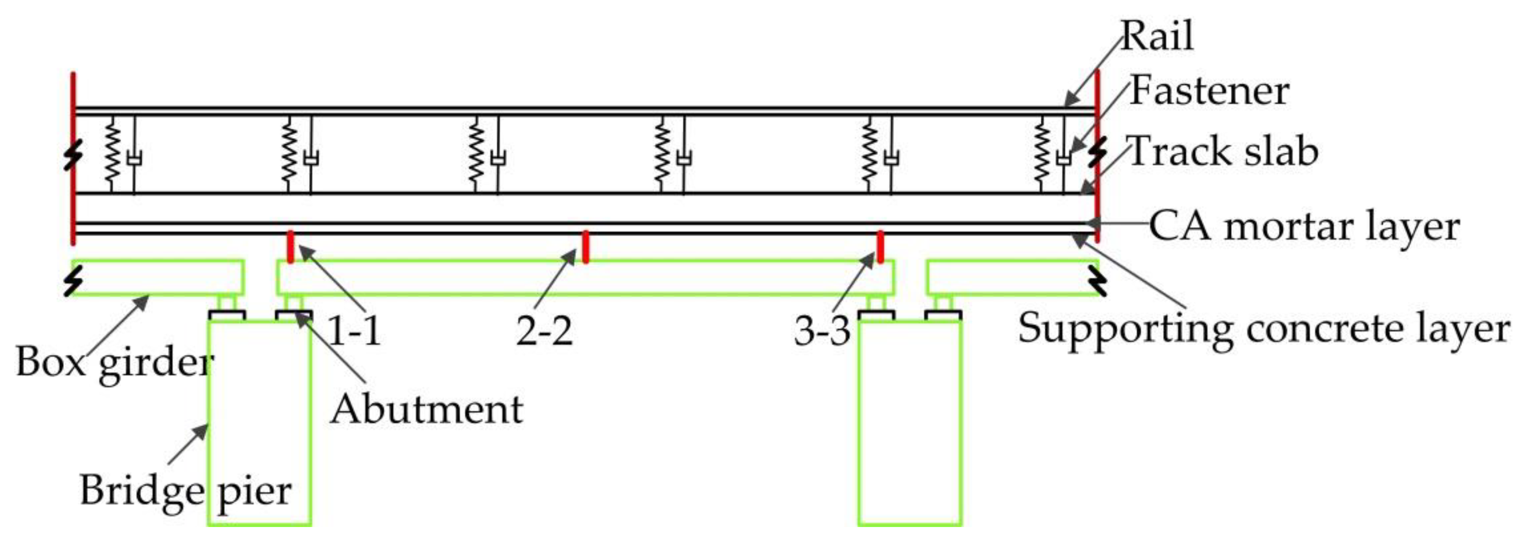
2. Monitoring Scheme

2.1. Instantaneous Baseline Establishment for Comparative Monitoring

Railway monitoring in the field is closely related to the form of track structure and foundation [48], temperature loads [49], train loads [50], and other factors. After communicating with the railway management and conducting on-site research and surveys for more than half a year, the authors found that two different segments in the same line at a distance of approximately 3 km had different chances to debond. Segment 1 was in a good state without debonding, while Segment 2 was in a poor state with slight debonding. The form of track structure and foundation are identical in two segments eliminating monitoring errors caused by differences in the form of structure. The track structure, which is composed of concrete, could lead to different temperature stresses when it is subjected to different temperature loads because of the thermal expansion and contraction effect, and therefore temperature loads have a significant impact on the monitoring. The monitoring errors caused by temperature loads may be introduced if the same zone is monitored at different times. In order to eliminate the influence of temperature loads on the monitoring results, comparative monitoring is carried out in two segments simultaneously. Due to the large variation in loads from one train to another, the use of comparative monitoring of two segments ensures consistency of train loads. In summary, the two segments are monitored simultaneously can eliminate errors introduced by structural differences, temperature loads, and train loads. At the beginning of the monitoring period, the differences between the parameters of the two segments were not significant, and as the monitoring time increased, the differences between the parameters of the two segments were large. This phenomenon indicates that Segment 1 is still in a good state, while Segment 2 has suffered from an interlayer debonding defect. As of May 2021, the track structure in Segment 1 was found to be still intact after a site survey, indicating that the monitoring system proposed in this paper was effective within a limited period of time.
Instead of using the conventional feature-comparison concept, which contrasts the current value of a feature with the historically pre-stored value of the same feature, this study builds an instantaneous baseline for diminishing the effects of varying environmental and operational conditions during the comparative analyses of debonding-associated features. Two CRTS-II-slab ballastless track segments of a standard simply-supported box-girder concrete viaduct in an in-service HSR were selected. Their cross-section sketch and longitudinal sketch are shown in Figure 1 and Figure 2. Figure 1 displays the cross-section of CRTS-II-slab ballastless track on a viaduct which is composed of rail, track slab, CA mortar layer, supporting concrete layer, and box-girder. Figure 2 shows three measurement positions of each track segment.
The two segments were intended to serve as a mutual instantaneous baseline for each other in feature comparison because they have the same structure and boundary conditions. In the early stage of monitoring, both Segment 1 and Segment 2 were in normal state, while Segment 2 seemed to have minor and negligible marginal debonding between track slab and CA mortar layer. The on-site monitoring system was implemented in January 2019. The early stage of monitoring included the first half-year in 2019, and the current stage of monitoring mentioned in this paper was from early October 2020. The vibration characteristics of Segment 1 and Segment 2 were analyzed to examine the effectiveness of instantaneous baseline. The high similarity between their vibration characteristics demonstrated that the two selected segments can be an instantaneous baseline for each other. If the feature values of one segment are significantly different from those of the other segment in the current stage, distinct damage may occur. The detailed validation process is described in Section 4.1. The interlayer debonding is a gap between track slab and CA mortar layer, longitudinally along the track slab in length, transversely along the track slab in width, and vertically along the track slab in height. The length of debonding is measured directly by a meter ruler. The end of the meter ruler is inserted into the gap until it stops moving; the scale of the meter ruler is the width of debonding. The height is measured by a thickness gauge, which consists of a number of pieces with different thicknesses, and the thickness of the piece inserted into the gap determines the height of debonding. In this manuscript, the debonding refers to the height of the interlayer debonding. As the structural inspection of the high-speed railway must be carried out in the skylight and the number of skylights is limited, we had to measure the size of the debonding at irregular intervals. A total of eight tests were carried out in March, June, August, October in 2019, and January, June, August, October in 2020. In October 2020, the health condition of Segment 2 had deteriorated, and the size of interlayer debonding in Segment 2 was about 6.45 m in length, the maximum height was about 2 mm (Figure 3), and the maximum width was about 155 mm. The location of the interlayer debonding was under a track slab near the middle of the viaduct. The discrimination of multiple time-domain, frequency-domain, and time–frequency features at cross-sections 1-1, 2-2, and 3-3 between the two segments will be examined in Section 4 to identify debonding-sensitive features and constructing a new indicator combining multiple debonding-sensitive features together.

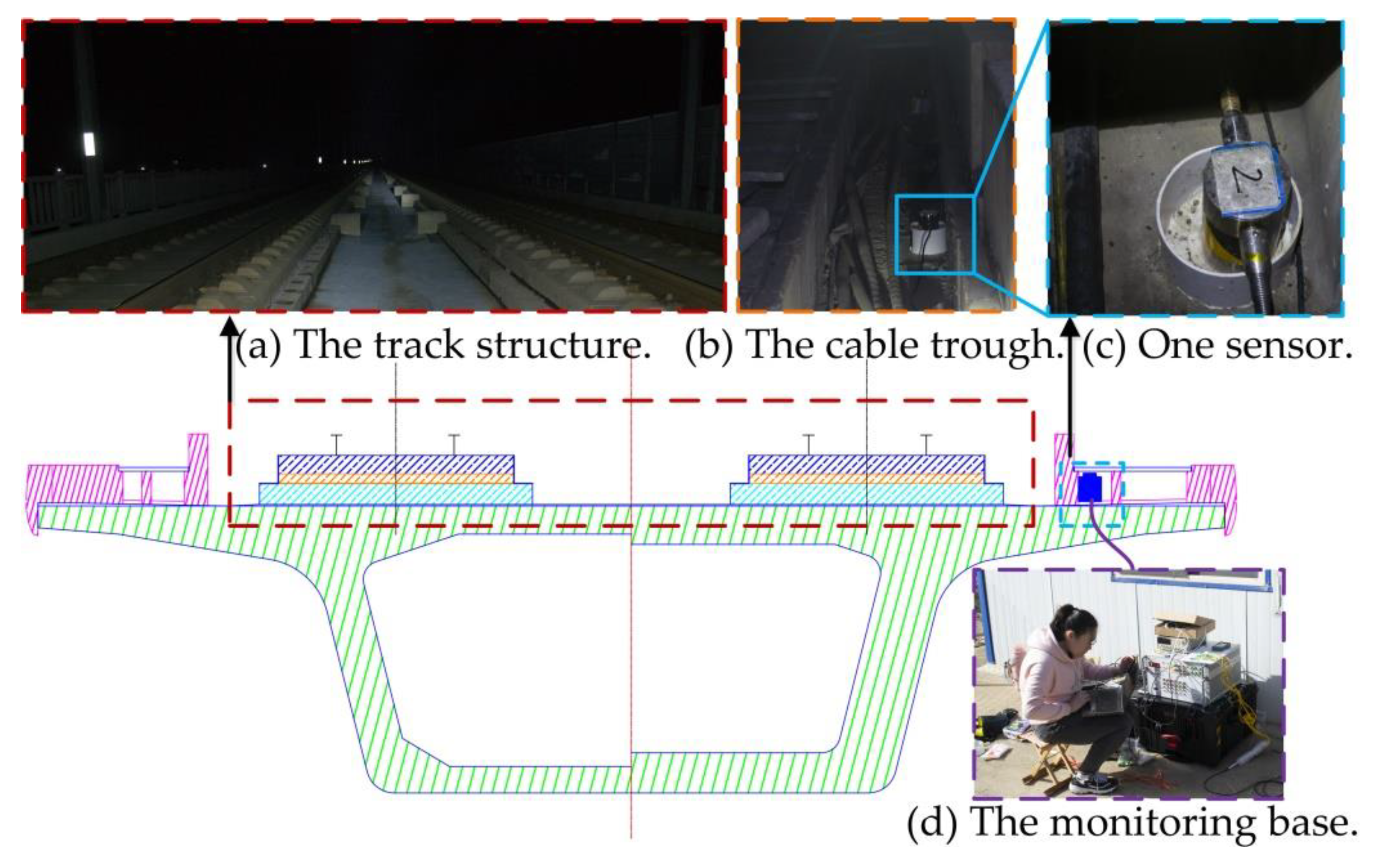
2.2. Fiber Optic Monitoring System and Deployment

The monitoring system shown in Figure 4 was adopted to establish a monitoring system that facilitates interlayer debonding detection, and its deployment is illustrated in Figure 5. The monitoring system mainly consisted of a signal generator, tunable laser, demodulator, and sensors. The selected sensors were interferometric fiber optic accelerometers with suitable bandwidth and high sensitivity [39]. Their sensitivity was tested to be 500 rad/g within the range of 0.1 to 1000 Hz. The measurement range was ±2 g. The interrogation of the interferometric fiber optic accelerometers in this paper was realized by the Phase Generation Carrier (PGC) demodulation technique [51]. The sampling frequency of the monitoring system was set to 1000 Hz.
In the field deployment scheme, there were six sensors in total for monitoring the two track segments. Three sensors were placed in the cable trough (Figure 5b) of each segment because the cable trough was the transversely nearest place to the debonding-prone area in the safety-securing zone allowed for sensor placement. As shown in Figure 2, the sensors were installed at the three cross-sections of each track segment. The white circular tube in Figure 5c was to prevent electric cables from touching the fiber optic accelerometers. The fiber optic transmission cable of the monitoring system was connected with the monitoring base (Figure 5d), which was about 1000 m away from the monitoring area, for signal demodulation and data accumulation.

3. Feature Extraction Methods and Indicator Development

3.1. Multi-Feature Extraction Methods in Time Domain

Six statistical methods were adopted, including clearance factor, crest factor, impulse factor, kurtosis factor, shape factor, and peak acceleration, to extract multi-perspective features in the time domain. The mathematical expressions and explanations of these statistical approaches are presented in Table 1. A comparative analysis between the baseline track segment without interlayer debonding and the track segment with interlayer debonding was performed, and the performance of time-domain features is assessed in Section 4.2.

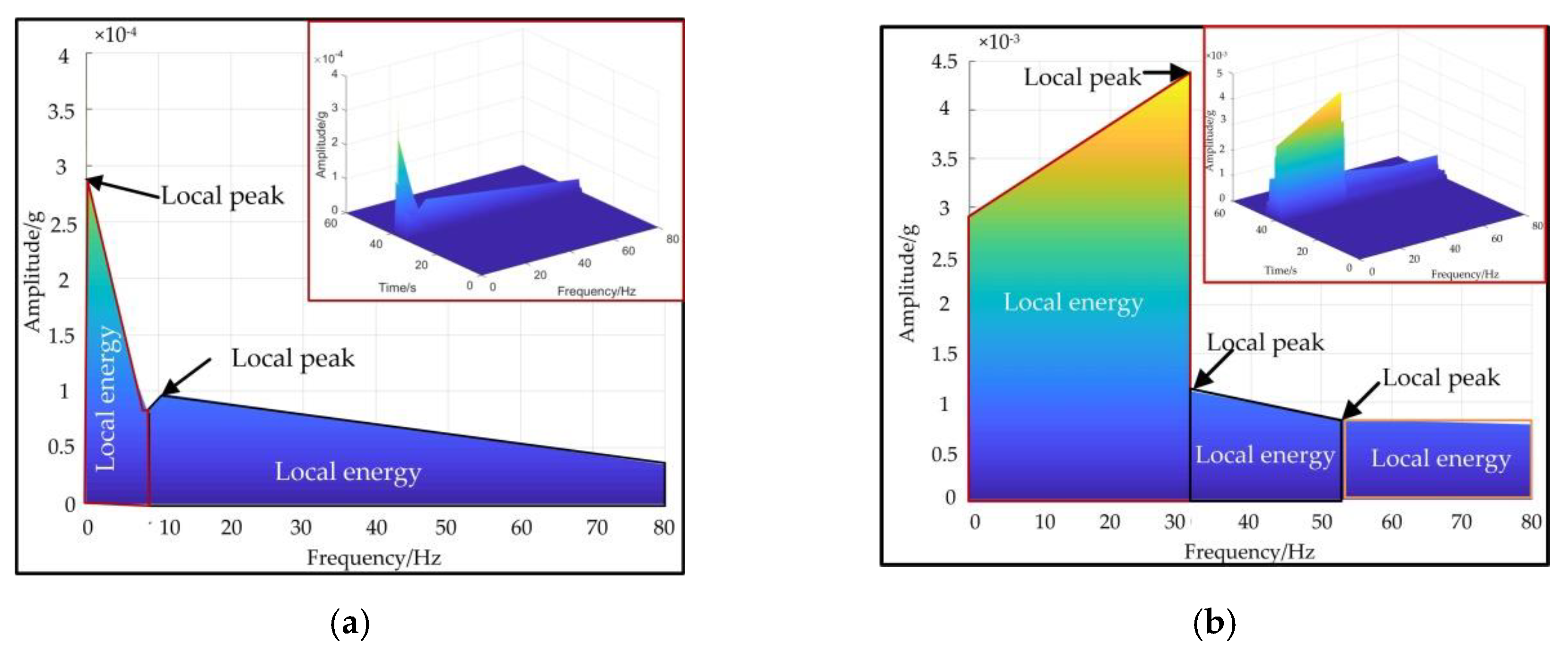
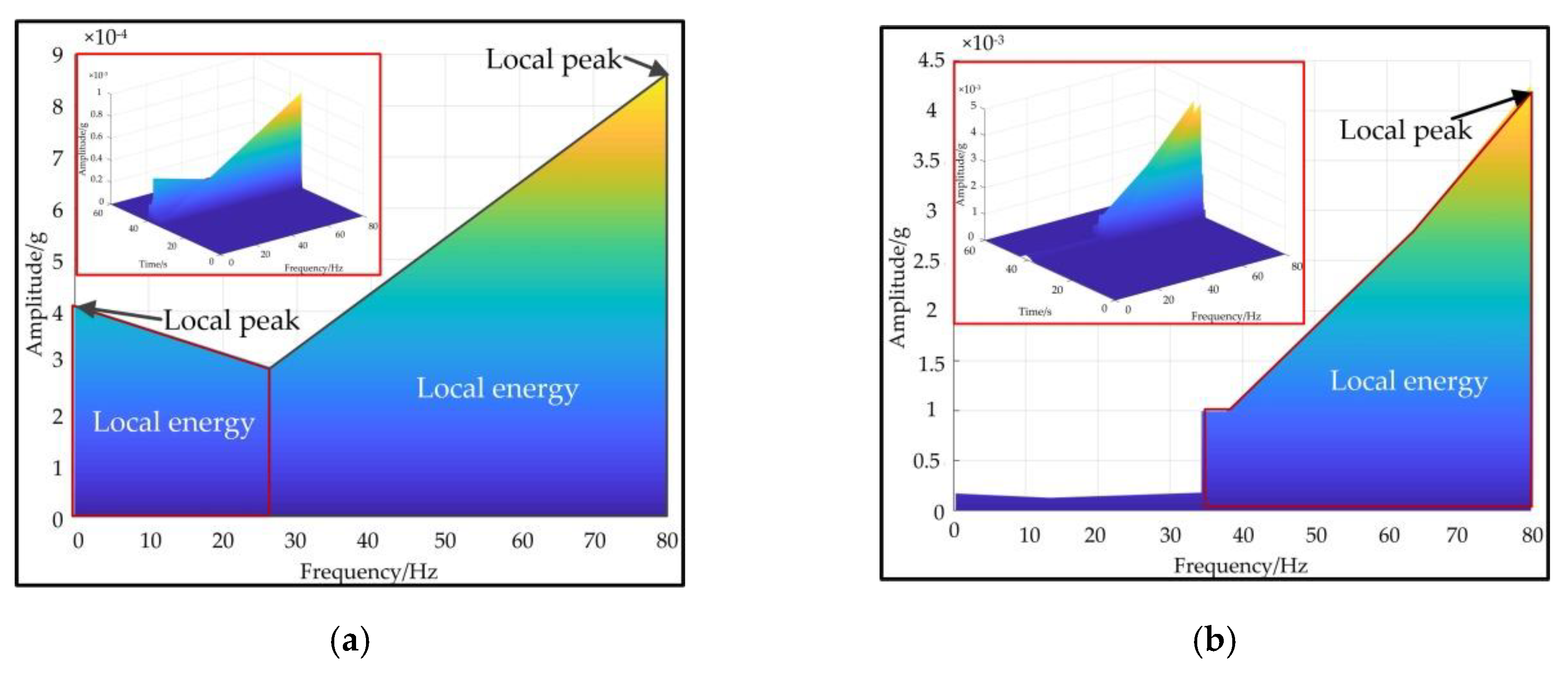
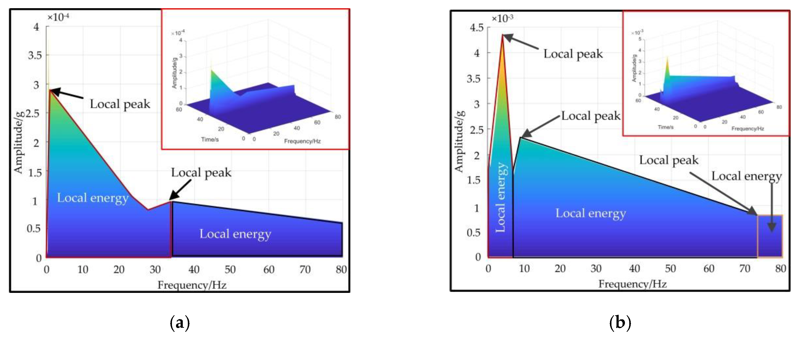
3.2. Multi-Feature Extraction Method in Frequency Domain

The fast Fourier transform method was employed to analyze the monitoring data acquired in normal state and interlayer debonding state to observe the changes in amplitude and frequency. This method was also used to extract the ground vibration caused by high-speed trains and analyze the vibration characteristics of ballastless track on bridges [44,45]. The mathematical expressions are presented in this section. A comparative analysis between the baseline track segment without interlayer debonding and the track segment with interlayer debonding was performed, and the performance of the frequency-domain features is assessed in Section 4.3.
The Fourier transform of a time-domain signal x(t) can be expressed as
X ( ω ) = + x ( t ) e j ω t d t
by which the continuous spectrum of the signal x(t) was calculated. However, in the actual monitoring system, discrete samples of continuous signals were obtained. The Discrete Fourier Transform (DFT) of a finite length discrete signal x(n), n = 0, 1, …, N − 1, is defined as
X ( k ) = n = 0 N 1 x ( n ) W N k n ( k = 0 ,   1 ,   ,   N 1 )
where W N = e j 2 π N . Using the symmetry and periodicity of WN, the DFT of N points is decomposed into two DFT with N/2 points, and the computational cost is reduced to half of the original.

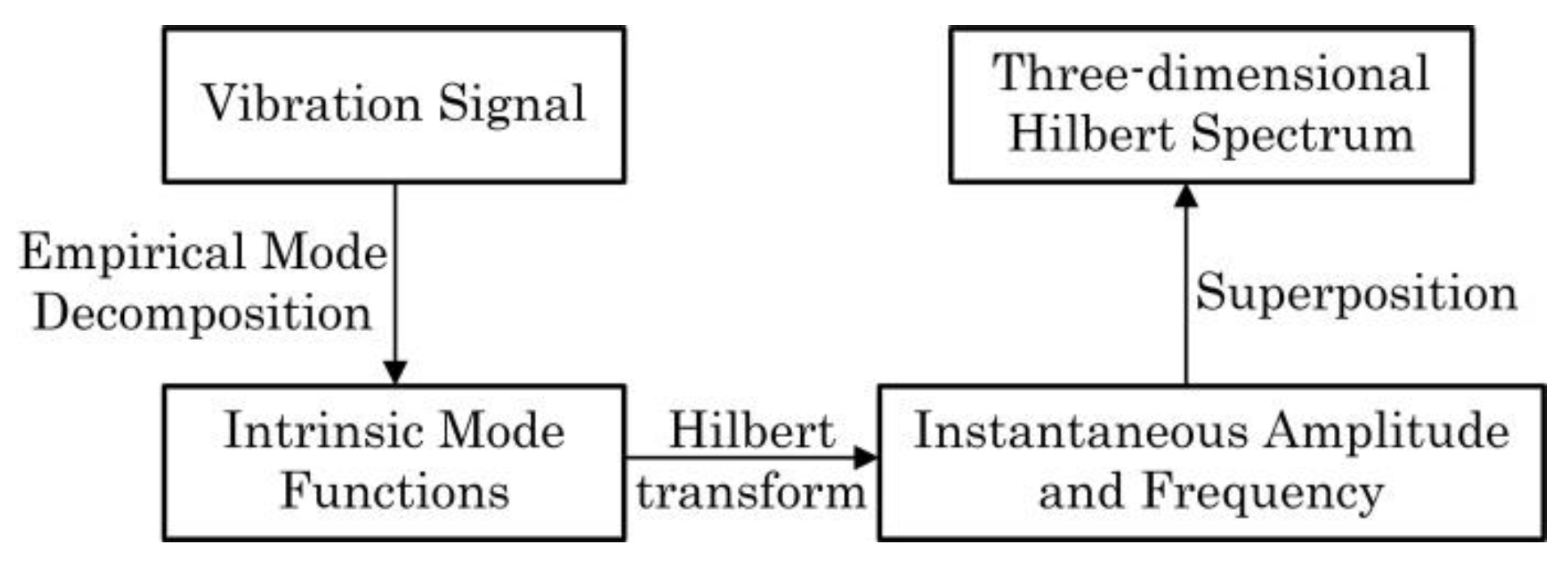
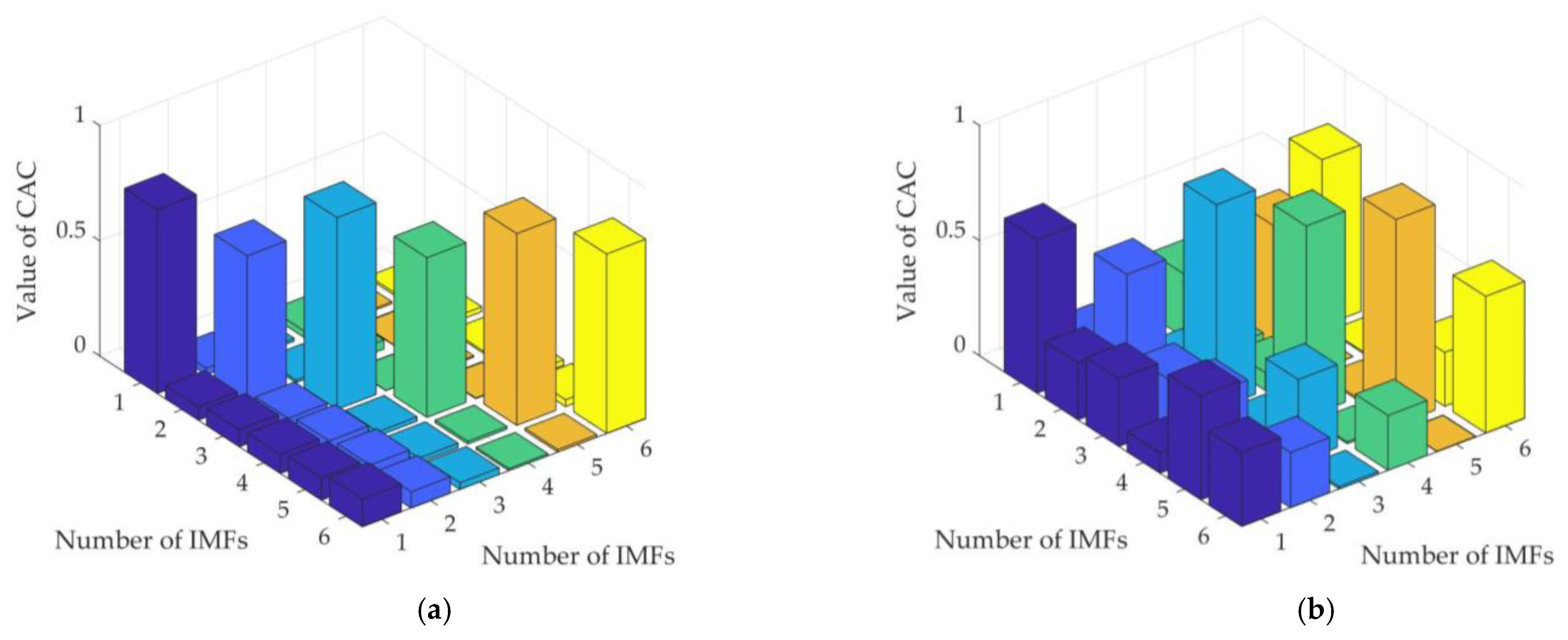
3.3. Multi-Feature Extraction Method in the Time–Frequency Domain

Track vibration is typically a nonstationary signal, and many scholars conduct time–frequency analysis for feature extraction. Zhang et al. [52] used short-time Fourier transform to analyze local deformation of HSR subgrade. Xu et al. [53] applied wavelet energy spectrum for track defect identification. Li et al. [54] adopted improved Empirical Mode Decomposition (EMD) to achieve the track irregularities detection. Chen et al. [55] applied EMD to diagnose the train wheel faults. HHT was applied for analyzing the damage-induced change in time-varying frequency and energy of rail structure [56].
To support the extraction of time–frequency features, such as local peak and energy in a frequency band, the HHT method [47], an adaptive time–frequency analysis method, was adopted. A comparative analysis between the baseline track segment without interlayer debonding and the track segment with interlayer debonding was conducted, and the performance of time–frequency features is evaluated in Section 4.4.
The flow chart of HHT is displayed in Figure 6. This algorithm starts with a temporally adaptive decomposition of a signal (i.e., EMD), producing a set of intrinsic mode functions (IMFs) and a remainder. On the basis of EMD, the original signal x(t) can be expressed in the following form:
x ( t ) = i = 1 n x i ( t ) + r ( t )
where xi(t) is the ith IMF and r(t) is the remainder. The Hilbert transform of the xi(t) is obtained by the following equation:
y i ( t ) = P π + x i ( τ ) t τ d τ
where P is the Cauchy principal value, yi(t) is the Hilbert transform of each IMF, and y(t) is obtained by superimposing the Hilbert transforms of all IMFs. Combining the x(t) and y(t), we can obtain the analytic signal z(t).
z ( t ) = x ( t ) + j y ( t ) = a ( t ) e i φ ( t )
a ( t ) = [ x 2 ( t ) + y 2 ( t ) ] 2 , ϕ ( t ) = arctan ( y ( t ) / x ( t ) )
where a(t) is the instantaneous amplitude of x(t) which can reflect the energy of x(t) varies with time, and φ(t) is the instantaneous phase of x(t).
One important property of the Hilbert transform is that if the signal x(t) is a mono-component, then the time derivative of instantaneous phase φ(t) is the instantaneous frequency ω(t) of the signal x(t).
ω ( t ) = d φ ( t ) d t
when the remainder is ignored, the original signal x(t) can be expressed as:
x ( t ) = Re i = 1 n A i ( t ) exp ( j w i ( t ) d t )
where ω(t) and Ai(t) are functions of time. By using HHT, rich information about frequency and amplitude can be obtained for further analysis. HHT is a time–frequency analysis method that can simultaneously obtain information about the time, frequency, and amplitude of a signal. In this study, three-dimensional time–frequency spectrums by HHT, which clearly show the change in frequency and amplitude, were obtained. In order to quantify the time–frequency spectrum, the front view of the three-dimensional time–frequency diagram is also displayed. The wheel–rail coupling system produces abnormal vibration in the debonding state which leads to a change in the waveform of the vibration, so it is necessary to focus on the amplitude of the vibration signal. Therefore, the local peak was one of the time–frequency domain indicators. Since the wheel–rail vibration in field has a large randomness, local energy was selected as one of the time–frequency domain characteristic indicators to eliminate uncertainty.
In addition to time–frequency features, the equation of MAC was introduced to calculate the relationship between any two dominant IMFs and generate more features. The term CAC (Equation (9)) replaces MAC to avoid confusion with the MAC in modal analysis.
C A C ( g , h ) = | x g T x h | 2 ( x g T x g ) ( x h T x h )   ( g = 1 ,   2 ,   ,   6 ;   h = 1 ,   2 ,   ,   6 )
where xg and xh represent the gth and hth IMF vector. A higher MAC value in modal analysis indicates a greater likelihood that the two modes belong to the same mode order. In this study, a higher CAC value represented a stronger correlation between two IMFs.

3.4. Development of a Similarity-Based Indicator

A new indicator was developed to quantify the feature difference between Segment 1 and Segment 2, which serve as a mutual instantaneous baseline for each other to combine debonding-sensitive features and realize comprehensive assessment. As formulated in Equation (10), the indicator is a weighted summation of p features. Since different features differ in contribution to the identification effect, weights were introduced to quantify the contribution of different features. The weight of each feature was calculated by normalizing the difference in feature values between the two segments in the early stage of monitoring.
F = b 1 f 1 + b 2 f 2 + + b l f l + + b p f p   ( l = 1 , 2 ,   ,   p )
The lth weight is expressed as b l = | f s e g 1 e a r l f s e g 2 e a r l | / l = 1 p | f s e g 1 e a r l f s e g 2 e a r l | . f s e g 1 e a r l represents the lth feature value of Segment 1, f s e g 2 e a r l represents the lth feature value of Segment 2 where l = 1 p b l = 1 . The superscripts ‘ear’ and ’cur’ denote the early stage and current stage of monitoring, respectively, and the subscripts ‘seg1’ and ‘seg2’ represent Segment 1 and Segment 2, respectively. The weights can characterize the importance of a feature to the identification, and the contribution to the identification increases with increasing weight. In the subsequent analysis, all of the adjustable constants were equal. The current values of the indicator for the two segments can be expressed as:
F s e g 1 c u r = b 1 f s e g 1 c u r 1 + b 2 f s e g 1 c u r 2 _ + + b p f s e g 1 c u r p
F s e g 2 c u r = b 1 f s e g 2 c u r 1 + b 2 f s e g 2 c u r 2 + + b p f s e g 2 c u r p
A significant difference between F s e g 1 c u r and F s e g 2 c u r implies that a distinct anomaly happens to one of the track segments, based on the assumption that the two track segments do not encounter damage at the same time.

4. Analysis and Discussion

The track monitoring was conducted for two years, demonstrating the applicability of the monitoring system and accumulating plenty of field monitoring responses. The responses excited by one type of vehicle was selected to reduce influential factors due to the different vehicle types in the subsequent analyses. This type of vehicle is characterized by eight carriages with two bogies and four wheelsets in each carriage. The axial distance between two wheelsets is 2.5 m, the central distance of two bogies is 17.5 m, and the whole length is 208.8 m. Generally, responses excited by a total of at least 39 trains of this type were recorded every day, and the passing-by speeds range from 71 km/h to 273 km/h. Before the subsequent analyses of these data, de-noising process of raw signals was performed. The ‘sym5′ wavelet function for multi-layer threshold de-noising [57] was employed in this paper. A typical raw signal before and after de-noising is shown in Figure 7. Figure 7b is an enlargement of the inset in Figure 7a. The blue and the red curves represent the raw signal and the de-noised signal, respectively. The correlation coefficient between raw signals and their de-noised signals was more than 0.95, so de-noised signals could be used for subsequent analyses. The analysis of historical data was performed at first to evaluate the reasonability of choosing the two segments as the mutual instantaneous baseline for each other. On this basis, comparative analyses between current features of Segment 1 and those of Segment 2 were conducted to identify the effective features which can distinctly differentiate interlayer debonding from the normal state.

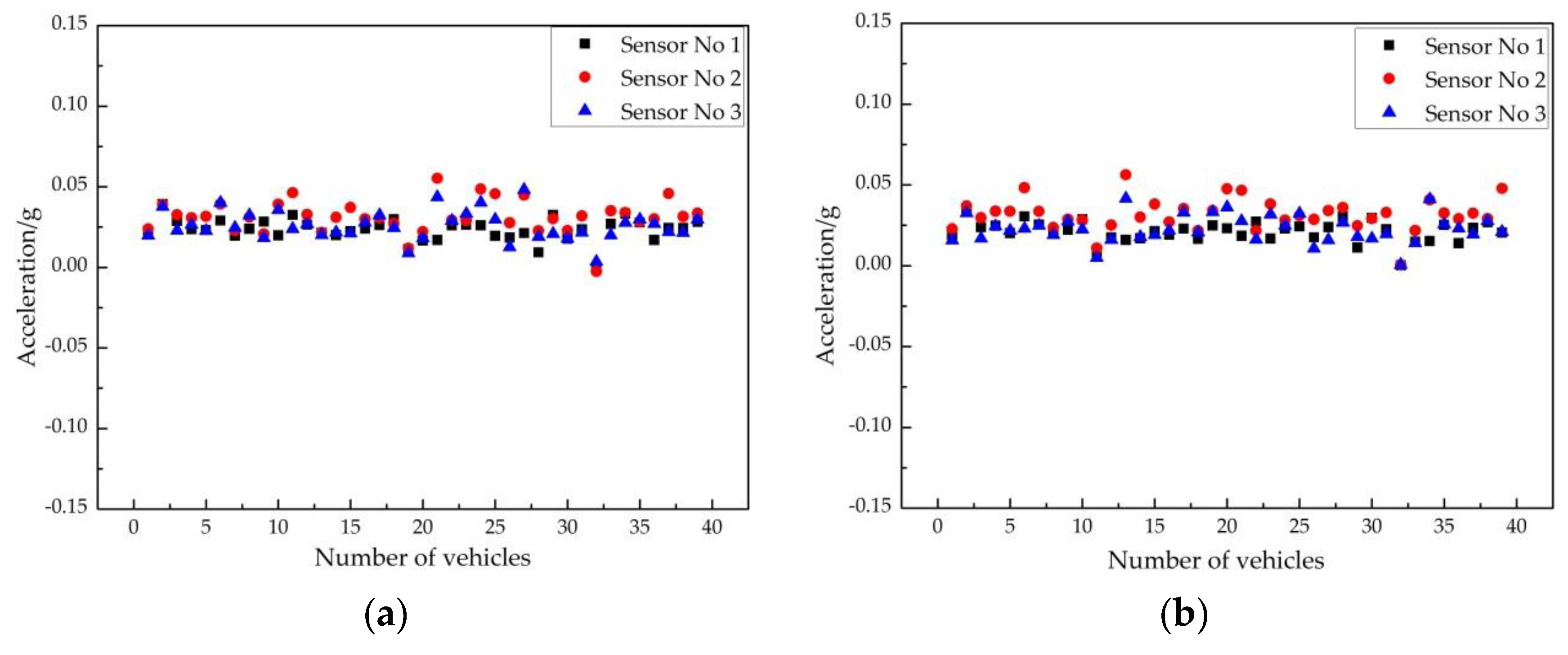
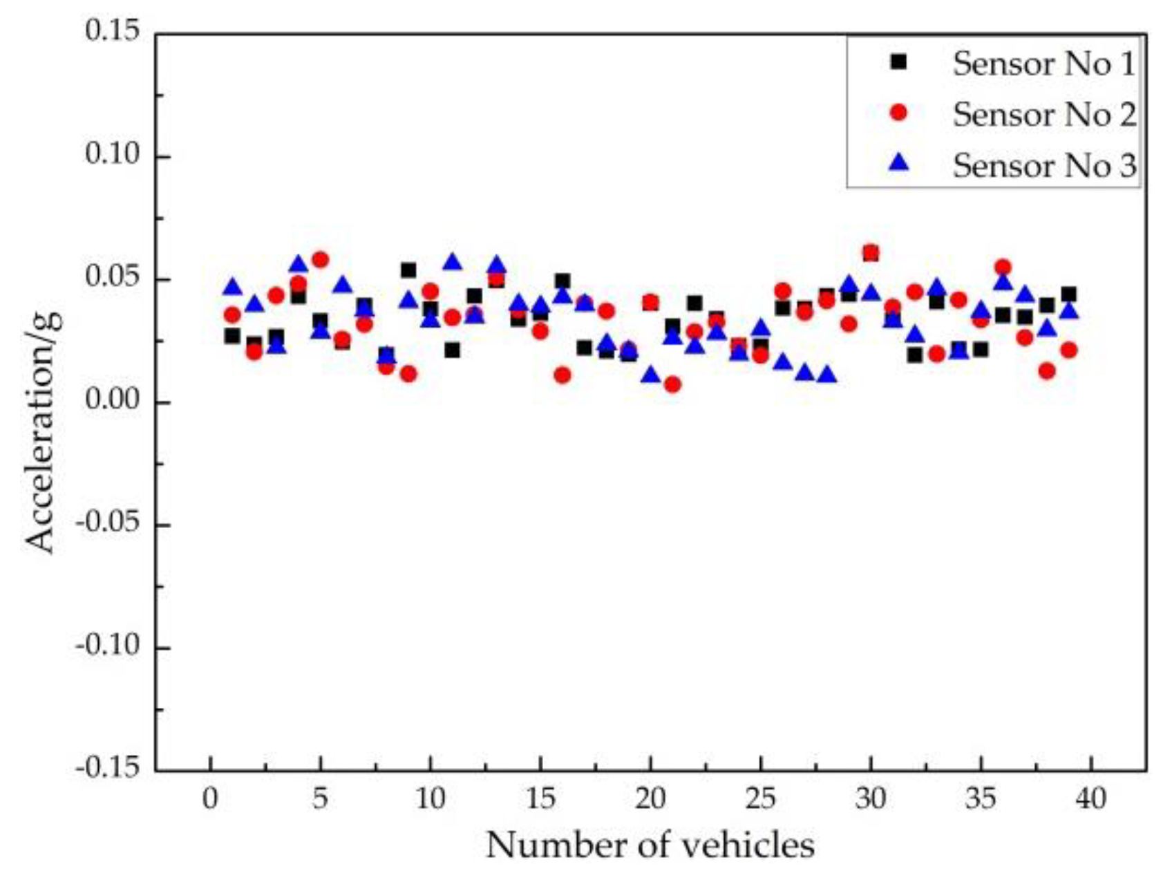
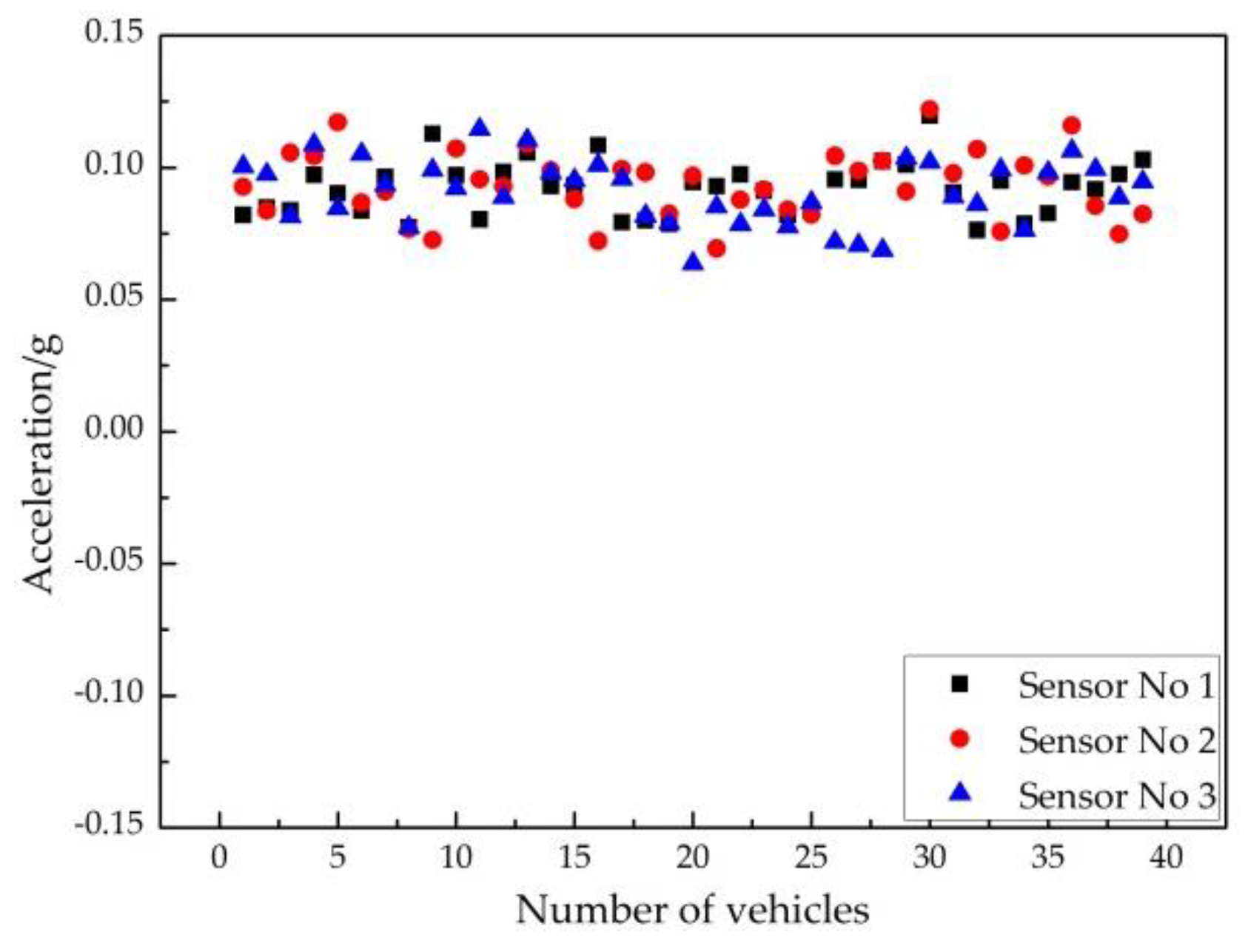
4.1. Validation of Instantaneous Baseline

In the early stage of on-site monitoring, both Segment 1 and Segment 2 were in a normal state, and Segment 2 seemed to have slight and negligible marginal debonding between track slab and CA mortar layer. The vibration characteristics of Segment 1 and Segment 2 were analyzed to examine the effectiveness of setting the two segments as mutual instantaneous baselines. The methods described in Section 3.1 were applied. The time-domain feature values are presented in this section, and the frequency-domain and time–frequency-domain feature values are omitted because their findings were accordant with those of the time-domain analysis. The six time-domain feature values and their differences between the two segments in the early monitoring stage are summarized in Table 2. Each value in this table is the average of all feature values of the responses from sensors No. 1–No. 3, induced by 39 passing-by vehicles in a typical day. The high similarity between their vibration characteristics demonstrates that the two selected segments could be an instantaneous baseline for each other.
Specifically, one of the time-domain features, peak acceleration, is illustrated in Figure 8 to observe their consistency. In Figure 8a,b, the horizontal coordinate displays the number of passing-by vehicles in a typical day, and the vertical coordinate exhibits the vertical acceleration of three sensors. The black rectangle and blue triangle represent the vertical accelerations of sensor No. 1 and sensor No. 3 in the cable trough of cross-sections 1-1 and 3-3 of the track segments, respectively, and the red circle stands for the vertical acceleration of sensor No. 2 in the cable trough of the cross-section 2-2 of the track segments. Figure 8a shows the scatter plot of the peak acceleration at the three measurement positions of Segment 1. Figure 8b shows the scatter plot of the same feature of Segment 2. The consistency in vibration levels between the two segments can be observed from Figure 8a,b.

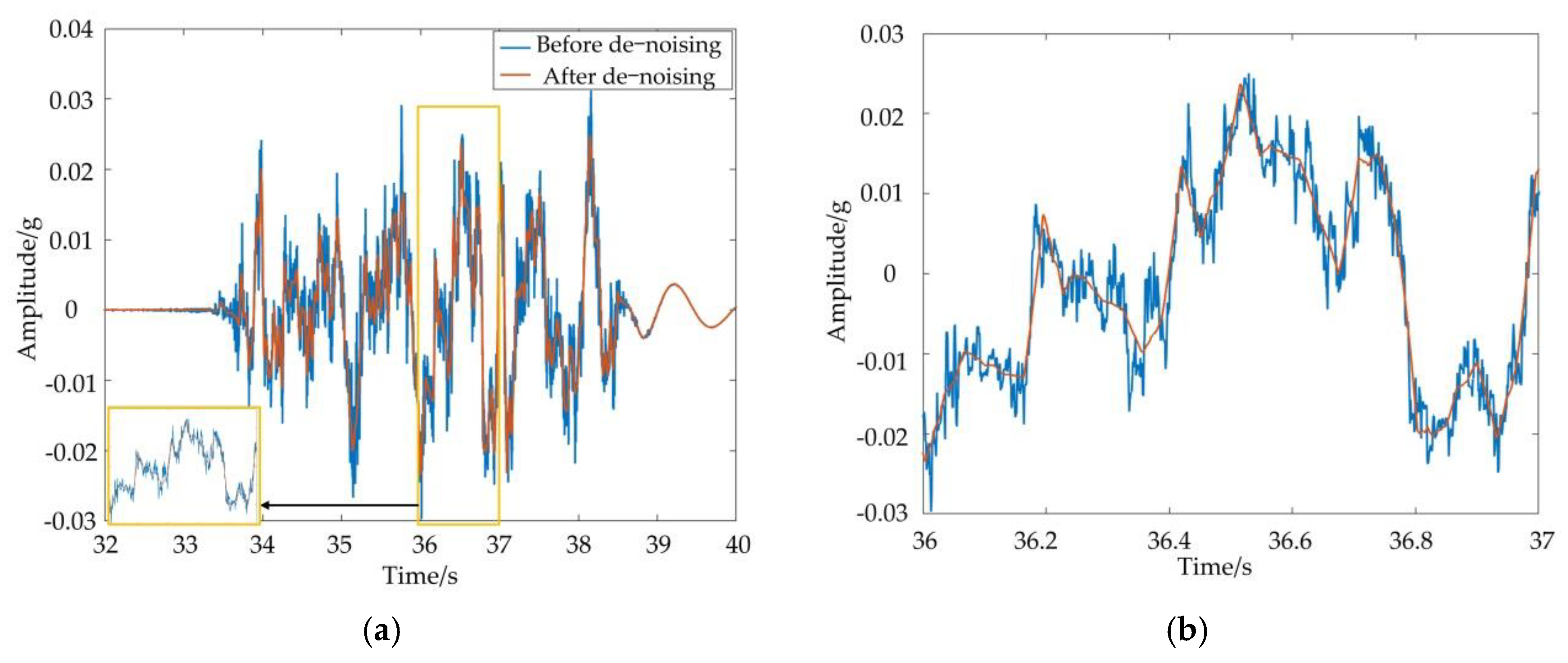
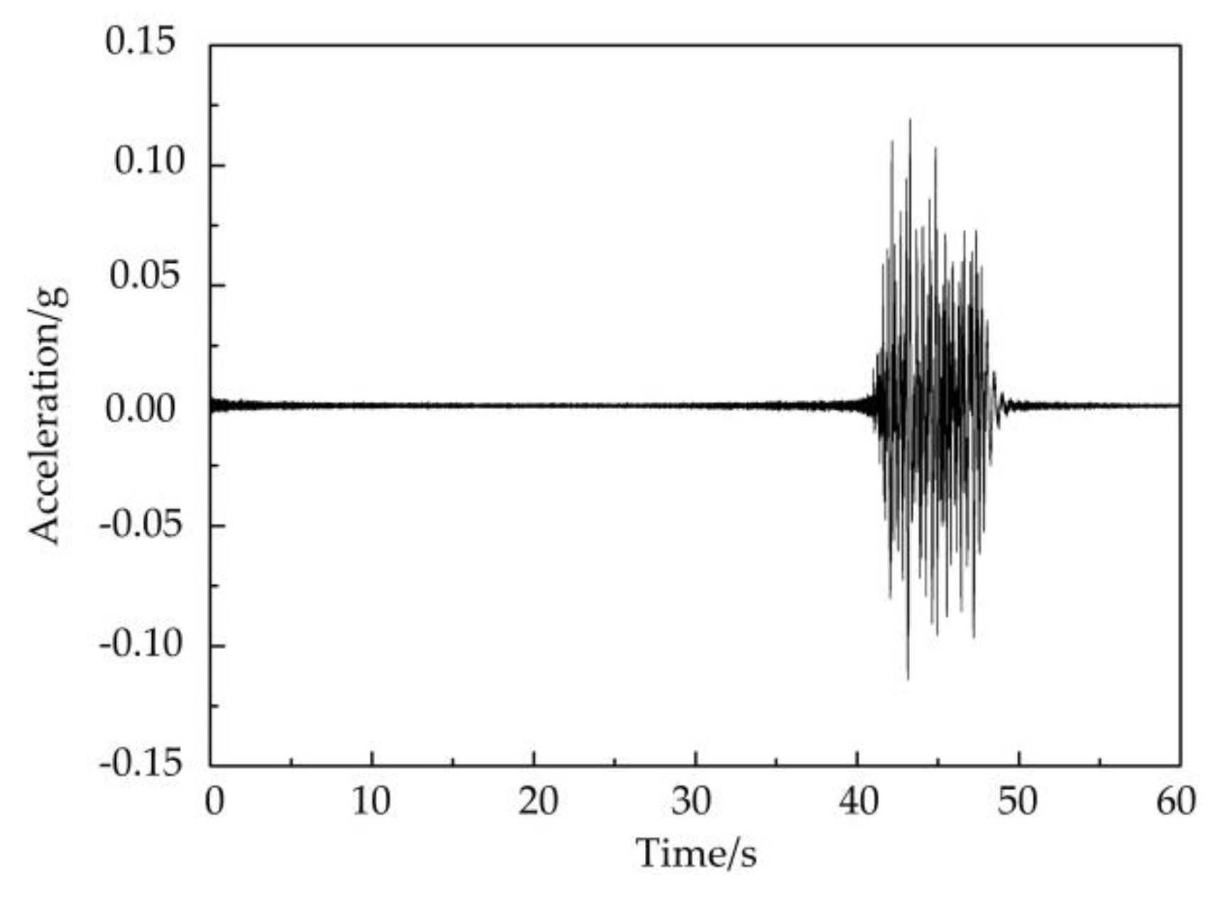
4.2. Time-Domain Analysis for Multi-Feature Extraction and Assessment

The health condition of Segment 2 was deteriorated, and it had a debonding of about 2 mm in thickness in the current monitoring stage after being subjected to train loads and environmental loads during long-term service. The discriminations between the time-domain features of the two track segments are shown in Table 3. Based on the mechanism of instantaneous baseline, if the features of one segment are significantly different from those of the other segment in the current monitoring stage, distinct damage may occur. From Table 2 and Table 3, it can be found: (i) compared to those in the early stage of monitoring, the relative differences of all the six time-domain parameters in the current stage of monitoring were larger, reflecting a debonding-induced change in responses; and (ii) the difference in peak acceleration in current monitoring stage was significantly higher than that in the early stage, indicating it is a dominant debonding-sensitive feature among the six features. Therefore, the peak acceleration feature was used in the subsequent analysis of Section 4.5. According to Table 1, these features were related to characteristics of response (i.e., the maximum, the mean value, and the RMS, etc.), so the reason for the enlarged differences between the early and current monitoring stages can be attributed to the debonding-induced stiffness reduction and the resultant change in track response.
Typical responses of Segment 1 and Segment 2 in the current stage of monitoring are illustrated in Figure 9 and Figure 10. The debonding-sensitive feature, peak acceleration, is illustrated in Figure 11 and Figure 12 to observe their discrimination. In Figure 11 and Figure 12, the horizontal coordinate displays the sequence number of passing-by vehicles in a typical day, and the vertical coordinate exhibits the vertical acceleration of three sensors. The black rectangle and blue triangle represent the vertical acceleration of sensor No. 1 and sensor No. 3 in the cable trough of cross-sections 1-1 and 3-3 of the track segments, respectively, and the red circle stands for the vertical acceleration of sensor No. 2 in the cable trough of the cross-section 2-2 of the track segments. It can be found by comparing Figure 11 and Figure 12 that the vibration level of Segment 2 was about three times higher than that of Segment 1, indicating the high sensitivity of this feature to debonding. The tolerable limit of peak acceleration of bridge deck on a viaduct of the ballastless track is 0.5 g [58], so both Segment 1 and Segment 2 were still in a safe state, although Segment 2 had a debonding of 2 mm in thickness. The CRTS-II-slab ballastless track system is famous for its low vibration and noise, but the vibration level has deteriorated due to the increased severity of debonding. Therefore, it is necessary to pay more attention to the track segment with debonding.

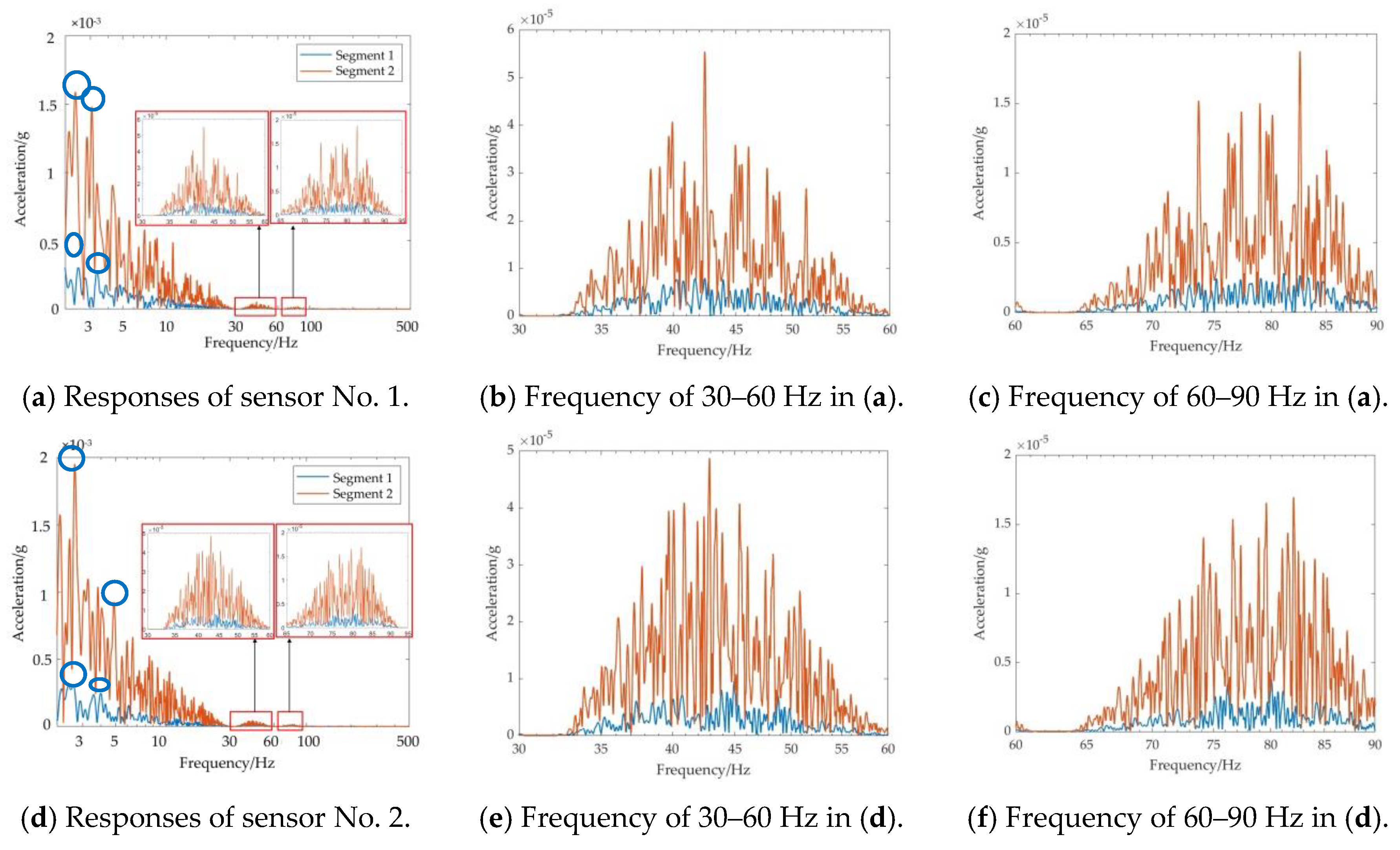
4.3. Frequency-Domain Analysis for Multi-Feature Extraction and Assessment

Previous studies have shown that the vibration frequency spectrum of the ballastless track of HSR changes when it is damaged [18,59]. In this section, the frequency spectrums of Segment 1 and Segment 2 are studied. Fourier transform was used to extract spectrum characteristics. The frequency-domain responses of Segment 1 and Segment 2 are shown in Figure 13, in which the blue line represents the spectrum of Segment 1, and the orange line stands for that of Segment 2. As the measurement positions at cross-sections 1-1 and 3-3 were symmetrical regarding the measurement position at cross-section 2-2, the spectrums of sensor No. 1 and sensor No. 3 were similar. As shown in Figure 13, the horizontal coordinate adopted a logarithmic scale, and the vibration energy was distributed in the frequency bands of 0~30 Hz, 30~60 Hz, and 60~90 Hz. The responses in 0~30 Hz accounted for the dominant proportion of energy, and the details of responses in 30~60 Hz and 60~90 Hz are also displayed in Figure 13a,i. Similar to the findings in Section 4.2, the vibration level of Segment 2 was considerably larger than that of Segment 1, which is consistent with the fact that Segment 2 had a distinct debonding defect.
Vibration is the cause of waves, and waves are the result of vibration. The low-frequency vibration in the manuscript is the wheel–track vibration wave reaching the cable trough after attenuation, and the frequency of the wheel–track vibration wave can reach 5 kHz [60], which is also a high-frequency wave like GWs [61]. The monitoring object is the China Railway Track System (CRTS)-II-slab ballastless track structure, which has a complex layer structure. The high-frequency wheel–rail vibration wave is attenuated through the CA mortar layer, which has the effect of vibration and noise reduction [3] to reach the cable trough to a low-frequency vibration wave. Further, the frequency of the vibration signal in the cable trough is concentrated within 100 Hz, as shown in Figure 13 and Table 4. This means that the wave used in this manuscript was also a high-frequency vibration wave. However, the ballastless track structure attenuates the high-frequency vibration wave to a low-frequency vibration wave. The authors in [62] conducted an in-depth study of damage detection of ballastless track structures by using low-frequency and high-frequency waves, respectively, and showed that high-frequency vibration waves with frequencies of 1–20 kHz are attenuated to 500 Hz when they pass through the track structure and reach the detection point. This is more consistent with the results of this manuscript and shows that the method proposed in this paper is reliable.
The peak frequencies and peak amplitudes of Segment 1 and Segment 2, marked by the blue circles in Figure 13a–c, are respectively listed in Table 4. The relative differences of peak frequencies and amplitudes between the two track segments are listed in the last column of these two tables. The peak frequencies of Segment 2 were slightly lower than those of Segment 1, and the peak amplitudes of Segment 2 were significantly higher than those of Segment 1. The reason for this phenomenon is that the stiffness of the ballastless track structure decreases due to the creation of interlayer debonding. As a result, the peak frequencies of the track structure decrease, and when subjected to the transient impact of passing-by trains, the vibration level of this track segment increases. These findings are coincident with the descriptions in [56]. The differences among the three graphs in Figure 13 may be ascribed to the longitudinal non-uniformity of the interlayer debonding thickness. The peak amplitudes exhibited obvious change, and this was similar to that situation in the time domain. The two features were able to distinguish interlayer debonding, so the peak frequency in the frequency domain was used as a feature for feature fusion.
It can be seen from Figure 13 and Table 4 that the vibration energy was concentrated in the frequency band of 0~30 Hz, and the peak frequencies were around 2.58 Hz and 3.68 Hz. The relationship between this phenomenon and the periodic excitation caused by the geometric characteristics of high-speed vehicles is explored in this part. The frequencies related to the geometric characteristics can be formulated as follows [63]:
f = v / L m   ( m = 1 ,   2 ,   3 ,   4 )
where v is the running speed of a passing-by high-speed vehicle, and Lm is a geometric characteristic of the vehicle. As shown in Figure 14, the lengths L1L4 were the distance between the two wheelsets of one bogie, the central distance between two bogies in a carriage, the distance between the front and rear bogies of two adjacent carriages, and the carriage length of the selected train type.
When the running speed was 232 km/h (measured by tachometer), the frequencies associated with the geometric characteristics were calculated by applying Equation (13) and listed in Table 5. The peak frequencies (around 2.58 Hz and 3.68 Hz) in Table 4 are ascribed to the two dominant geometric characteristics L4 and L2 in Table 5. The geometric-characteristics-related frequencies, namely 2.58, 3.68, 8.59, and 25.78 Hz, contributed to the energy concentration in 0~30 Hz. The measured frequencies deviated from these characteristic frequencies, and this may result from the Doppler effect happening when a high-speed train is approaching or leaving the measurement positions.
The vibration acceleration level [64] can reveal the vibration level of a structure. The formula of the vibration acceleration level VAL is shown in Equation (14):
V A L = 20 log a a 0
where VAL is vibration acceleration level (dB); a is the effective value of vibration acceleration (m/s2); a0 is the base acceleration, which is taken as 10−6 m/s2.
As can be seen from Table 6, the vibration level of Segment 2 was larger than that of Segment 1, indicating that the vibration response of the track structure increased significantly when the track structure was in an interlayer debonding state. In addition, there was little difference in the vibration level between sensor No. 1 and sensor No. 3 regardless of the segment, owing to the fact that sensor No. 1 and sensor No. 3 were both located at the end of the viaduct. The vibration level of sensor No. 2 was greater than that of sensors No. 1 and 3 in that sensor No. 2, which was located in the middle of the viaduct, vibrated larger than the end of the viaduct when subjected to train loads. This also verifies that the monitoring system proposed in this manuscript is accurate.

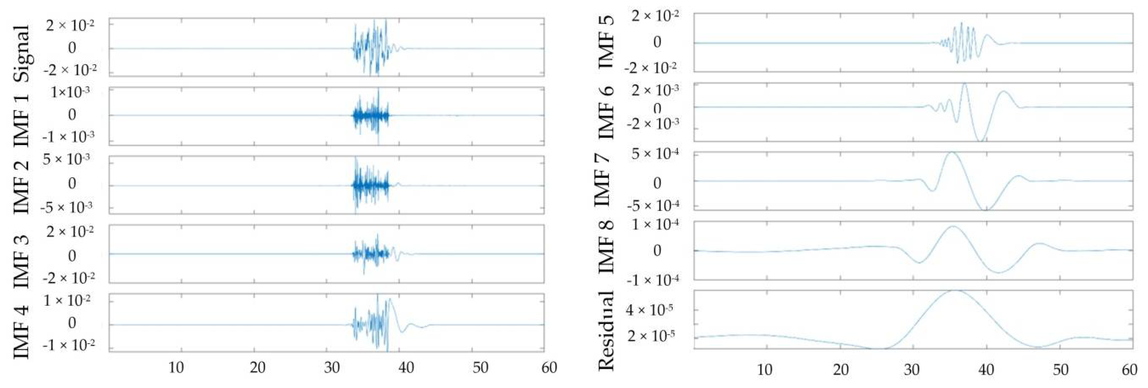
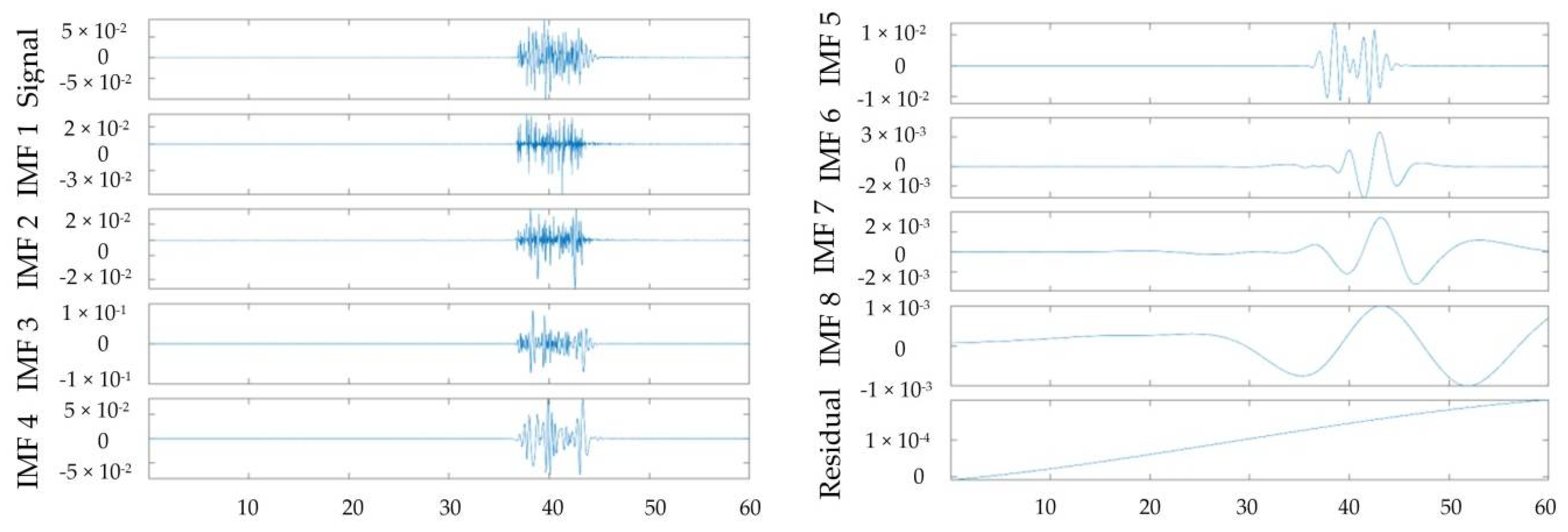
4.4. Time–Frequency-Domain Analysis for Multi-Feature Extraction and Assessment

Time–frequency analysis of current data was conducted by using the HHT method described in Section 3.3. The IMFs of a typical response of Segment 1 and those of Segment 2 are shown in Figure 15 and Figure 16. The correlation coefficient is a quantity that examines the degree of linear correlation between variables. The formula for the correlation coefficient between one IMF and the original signal is:
r ( x i , x ) = C o v ( x i , x ) V a r ( x i ) V a r ( x )
where xi denotes the ith IMF vector, x denotes the vector of the original signal, Cov(xi,x) is the covariance of xi and x, Var(xi) is the variance of xi, and Var(x) is the variance of x.
In Figure 15 and Figure 16, IMF1-IMF8 represents the eight IMFs obtained by using EMD of the original signal, and the residual are the remaining components. The correlation coefficients between IMF1~IMF8 and the original signal were −0.0639, 0.1293, 0.5204, 0.3890, 0.6243, 0.0028, −1.1562 × 10⁻⁴, and −1.9159 × 10⁻⁴. Since the correlation coefficients of the first six orders of IMF were larger, the Hilbert transform was performed by using IMF1~IMF6. In Figure 16, the correlation coefficients of eight IMFs were 0.0586, 0.3286, 0.6378, 0.4109, 0.0200, −7.541 × 10⁻⁴, −3.8681 × 10⁻⁴, and 1.9866 × 10⁻⁵, respectively, so the time–frequency response was obtained by the Hilbert transform with the use of IMF1~IMF5.
The results of HHT are depicted in Figure 17, Figure 18 and Figure 19. The changes in local peaks and energy in different frequency bands shown in these figures are summarized in Table 6. Energy is represented by the colored area above the coordinate axis. The local peak is the maximal value of amplitude in a frequency band. It can be seen that the energy distribution of Segment 2 was significantly different from that of Segment 1 at all measurement positions. Energy-concentration frequency bands changed, and local peaks and energy were higher due to the debonding. Specifically, the main energy-concentration area of sensor No. 1 was shifted from 0~10 Hz to 0~35 Hz, and the local peak and energy of this sensory signal had a drastic rise with the occurrence of the debonding. Similar changes happened in the response of sensor No. 3. The main energy-concentration area of sensor No. 2 was shifted from 0~80 Hz to 36~80 Hz, and the local peak and energy of this sensor also witnessed significant increases, accompanied by the occurrence of debonding. In the main energy-concentration area, the local peak and energy of Segment 2 (in the debonding state) were 10 and 14 times higher than those of Segment 1 (in normal state), respectively. The features in Table 7 include the maximum local peak and the maximum local energy from one of the three sensors, and their relative differences is listed in the last column in this table. According to Table 7, it was found that the local peak, local energy, maximum local peak, and maximum local energy experience significant increased accompanied by the occurrence of debonding. Therefore, the features in time–frequency domain are effective in differentiating debonding state from the normal state.
Further, the CAC values among the first six IMFs of Segment 1 and those of Segment 2 were calculated by using Equation (9) in Section 3.3. The CAC values of Segment 1 and Segment 2 in the current stage of monitoring are shown in Figure 20. The CAC represents the degree of correlation between two IMFs. When the track structure is in a state of interlayer debonding, the wheel–rail vibration signal waveform will definitely change. The change in signal leads to a change in IMF and, therefore, a change in CAC mode. Compared to the normal state of the track structure, interlayer debonding results in more reflective surfaces in the propagation path of the vibration, and thus the vibration signal is complicated. As can be seen by comparing Figure 20a,b, the interlayer debonding led to a complex CAC pattern. By comparing Figure 20a,b, it was found that the CAC pattern of Segment 2 obviously deviated from that of Segment 1, which is accordant to the fact that Segment 2 is in a debonding state while Segment 1 is in a normal state. The CAC pattern (the group of 36 CAC values) is also debonding-sensitive. In time–frequency-domain feature extraction, the CAC deviation from diagonal matrix was more sensitive to interlayer debonding defect because of neglecting the higher diagonal, which is named as active CAC instead of CAC as time–frequency-domain feature. The maximum ones among the local peaks and local energies in different frequency bands in Table 6 and this group of CAC values were used in the subsequent analysis of Section 4.5.

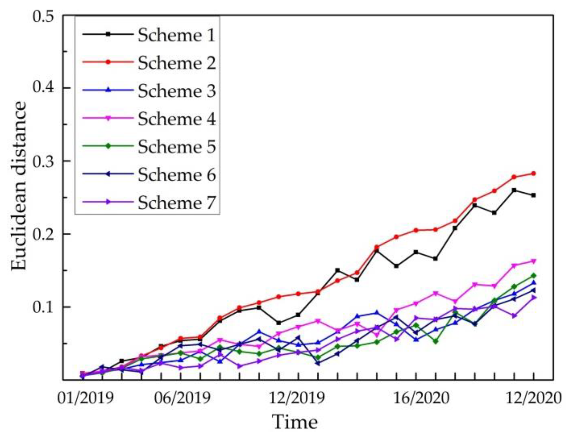
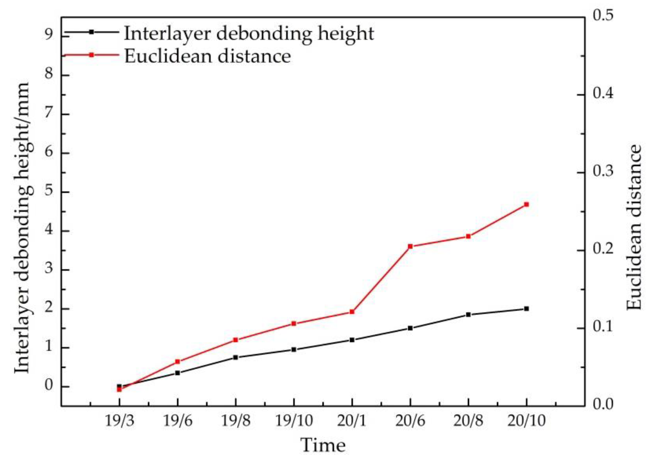
4.5. Quantitative Assessment Using the Similarity-Based Indicator

In order to study the influence of feature selection on recognition results, different features in time domain, frequency domain, and time–frequency domain were selected for fusion, and a total of seven features fusion methods were established, as shown in Table 8. Scheme 1 is the baseline. Scheme 2 verifies the recognition effect of active CAC features, Schemes 3–4 verify the recognition effect of the time-domain feature and frequency-domain feature, respectively, and Schemes 5–7 verify the recognition effect of time–frequency-domain features, respectively. The values of the proposed indicator for Segment 1 and Segment 2, which serve as mutual instantaneous baselines, F s e g 1 and F s e g 2 , were calculated with the use of Equations (11) and (12) in Section 3.4. The time histories of F s e g 1 and F s e g 2 , together with their Euclidean distance of Scheme 1, are plotted in Figure 21. The red and black curves represent the indicator values of Segment 1 and Segment 2, and the blue curve is the Euclidean distance quantifying the feature difference between the two segments. It can be found that the two curves for F s e g 1 and F s e g 2 were coincident with each other in the early stage of monitoring and later F s e g 1 fluctuated stably while F s e g 2 had a continuous increase. The Euclidean distance between them gradually enlarged, which implies that Segment 2 suffered from an anomaly (i.e., debonding in this case), and the severity level of the anomaly had been continuously aggravated. This is coincident with the occurrence and deterioration of interlayer debonding of the monitored track system.
Seven features fusion methods differed in the effect of identifying interlayer debonding, and the identification results are shown in Figure 22. In the figure, it can be seen that seven features fusion methods were able to characterize the increase in interlayer debonding with time, indicating that the proposed method in this manuscript does not depend on feature selection. However, different feature fusion methods differed in the identification effect. Compared with Scheme 1 (black curve), Scheme 2 (red curve) was flatter, less fluctuating, and had the most significant increase, so Scheme 2 has the best recognition. There was little difference in the recognition effect of Scheme 3–Scheme 7.
The contribution of different features which differ in the recognition effect is characterized by the weight index. The weights of different features in seven features fusion methods are shown in Table 9. The contribution to the identification of interlayer debonding increased with increasing weight. In Table 9, it can be seen that time–frequency-domain features contributed the most to the identification effect, accounting for more than 50%, and the time-domain features contributed more than the frequency-domain features.
In addition, the sensitivity of seven features fusion methods was calculated by referring to the calculation method of feature sensitivity in [65], and the results are shown in Table 10. The higher the sensitivity, the better the recognition effect of the feature’s fusion methods. In Table 10, the sensitivity of the seven features fusion methods is ranked as follows: 2 > 1 > 4 > 3 > 5 > 6 > 7, indicating that Scheme 2 had the best recognition effect and Scheme 7 had the weakest recognition effect.
A comparison between the interlayer debonding and Euclidean distance versus time by using scheme 2 was analyzed to investigate the relationship between them, and the results are shown in Figure 23. In Figure 23, the black and red curves represent the variation of debonding and the Euclidean distance with time, respectively. The value of the debonding increased slowly with time, indicating that the interlayer debonding was expanding. The Euclidean distance showed an increasing trend, indicating that the Euclidean distance increased with the interlayer debonding.

5. Conclusions

In this study, the interlayer-debonding monitoring of a new-type track structure, CRTS-II-slab ballastless track, was investigated for supporting debonding identification and assessment. The monitoring framework targeting this issue was built in this study, which included three parts: (i) a monitoring scheme with instantaneous baseline and trackside sensor deployment near the debonding-prone area to facilitate interlayer debonding detection; (ii) a fiber optic system used for implementing the monitoring scheme and continuously capturing the low-frequency small-amplitude acceleration at the measurement positions; and (iii) multiple features characterized by easy implementation and fast calculation and a new indicator combining debonding-sensitive features for identifying and assessing interlayer debonding. The monitoring scheme with the design of mutual instantaneous baselines and trackside sensor deployment near the bonding-prone area was developed to facilitate its interlayer debonding detection and diminish the effects of varying environmental and operational conditions on feature and indicator comparison. With the application of the monitoring scheme to the CRTS-II-slab ballastless track on a viaduct in an in-service high-speed rail line, field monitoring data were continuously acquired by a high-sensitivity fiber optic monitoring system over the past two years. After validating the effectiveness of setting two identical segments of the track as mutual instantaneous baselines, multiple feature-extraction techniques characterized by easy implementation and rapid calculation were employed to differentiate the track segment with interlayer debonding from another track segment in a normal state. Six features in the time domain, two features in the frequency domain, and more than thirty features in the time–frequency domain were extracted. The reasons associated with specific vibration characteristics were explained. By performing seven feature fusion methods, it was found that Scheme 2 exhibited high sensitivity to debonding. Moreover, a new indicator, combining multiple debonding-sensitive features by similarity-based weights normalizing the initial difference between mutual instantaneous baselines, was developed to support rational and comprehensive assessment of interlayer debonding quantitatively. Euclidean distance between the indicator curves of the two track segments of the seven features fusion methods both had a continuous increase, which was coincident with the occurrence and deterioration of interlayer debonding. This study is conducive to the establishment of an effective feature pool and a new indicator for rapid debonding identification and assessment of track system and thus contributes to the safety of train operation and the comfort of passengers. Extensive investigations into the SHM of the ballastless track exist, but the study on this type of interlayer-debonding monitoring scheme and its application to the debonding identification of an in-service HSR track with the assistance of the new indicator is rarely reported. The difficulties for generalizing this work to other applications are the establishment and validation of mutual instantaneous baselines and the development of a damage-sensitive indicator with the mechanism able to normalize initial error between the mutual instantaneous baselines.

Author Contributions

Conceptualization, G.G. and J.W., Methodology, J.W., Formal analysis, G.G., Investigation, G.G., Resources, G.G., Writing-Original draft, G.G., Writing—Review & Editing, G.G. and J.W., Supervision, B.D. and Y.D. All authors have read and agreed to the published version of the manuscript.

Funding

This research was funded by the National Key R&D Program of China (2019YFB2102702 and 2018YFB2101003), National Natural Science Foundation of China (52008258, 51991395, 51822802, 51778033, U1811463, 71901011, and 51808359), the Science and Technology Major Project of Beijing (Z191100002519012), Shenzhen Science and Technology program (KQTD20180412181337494), China Railway Corporation Science and Technology Research and Development Project (P2018G005-2), Guangdong Provincial Science and Technology Plan Project (Grant No. 2018B020207011).

Data Availability Statement

The raw data required to reproduce these findings cannot be shared at this time as the data also forms part of an ongoing study.

Acknowledgments

The authors thank Wentao Zhang at Semiconductor Research Institute of Chinese Academy of Sciences for his provision of optical fiber sensing equipment, thank Xuhao Cui at School of Engineering, Beijing Jiaotong University, for supporting field investigation, and thank Fei Xu at Structural Health Monitoring and Control Institute, Shijiazhuang Tiedao University, for providing resources to support data analysis.

Conflicts of Interest

The authors declare no conflict of interest.

References

  1. Zhang, N.; Guo, W.W.; Xia, H. Dynamic Interaction of Train-Bridge Systems in High-Speed Railway, 1st ed.; Beijing Jiaotong University Press: Beijing, China, 2018; Volume 1, pp. 13–14. [Google Scholar]
  2. Luo, J.; Zhu, S.Y.; Zhai, W.M. An efficient model for vehicle-slab track coupled dynamic analysis considering multiple slab cracks. Constr. Build. Mater. 2019, 215, 557–568. [Google Scholar] [CrossRef]
  3. Wang, P.; Xu, H.; Chen, R. Effect of cement asphalt mortar debonding on dynamic properties of CRTS-II- slab ballastless track. Adv. Mater. Sci. Eng. 2014, 8, 193128. [Google Scholar] [CrossRef] [Green Version]
  4. Shi, H.; Yu, Z.J.; Shi, H.M.; Zhu, L.Q. Recognition algorithm for the disengagement of cement asphalt mortar based on dynamic responses of vehicles. Proc. Inst. Mech. Eng. Part F J. Rail Rapid Transit 2019, 233, 270–282. [Google Scholar] [CrossRef]
  5. Yu, C.Y.; Xiang, J.; Mao, J.H. Influence of slab arch imperfection of double-block ballastless track system on vibration response of high-speed train. J. Braz. Soc. Mech. Sci. 2018, 109, 1–14. [Google Scholar] [CrossRef]
  6. Ke, Y.T.; Cheng, C.C.; Ni, Y.Q.; Hsu, K.T.; Wai, T.T. Preliminary study on assessing delaminated cracks in cement asphalt mortar layer of high-speed rail track using traditional and normalized impact—Echo methods. Seonsors 2020, 30, 3022. [Google Scholar] [CrossRef]
  7. Hoda, A.; Soheil, N.; Deren, Y. Assessing sensitivity of impact echo and ultrasonic surface waves methods for nondestructive evaluation of concrete structures. Constr. Build. Mater. 2014, 71, 384–391. [Google Scholar]
  8. Taekeun, O.; Jongil, P. Comparison of Data-Processing Methods by Air-Coupled Impact Echo Testing for the Assessment of a Concrete Slab. J. Test Eval. 2014, 42, 921–930. [Google Scholar]
  9. Lutz, A.; Samir, S. Track-Soil Dynamics-Calculation and Measurement of Damaged and Repaired Slab Tracks. Transp. Geotech. 2017, 12, 1–14. [Google Scholar]
  10. Xu, J.M.; Wang, P.; Liu, H. Identification of internal damage in ballastless tracks based on Gaussian curvature mode shapes. J. Vibroeng. 2016, 18, 1392–8716. [Google Scholar]
  11. Nikolaos, Z.; Efthymios, T.; Christos, V. Inspection, evaluation and repair monitoring of cracked concrete floor using NDT methods. Constr. Build. Mater. 2013, 48, 1302–1308. [Google Scholar]
  12. Che, A.L.; Tang, Z.; Feng, S.K. An elastic-wave-based full-wavefield imaging method for investigating defects in a high speed railway under track structure. Soil Dyn. Earthq. Eng. 2015, 77, 299–308. [Google Scholar] [CrossRef]
  13. Varnavina, A.V.; Khamzin, A.K.; Torgashow, E.V. Data acquisition and processing parameters for concrete bridge deck condition assessment using ground-coupled ground penetrating radar: Some considerations. J. Appl. Geophys. 2015, 114, 123–133. [Google Scholar] [CrossRef]
  14. Yang, Y.; Zhao, W.G. Curvelet transform-based identification of void diseases in ballastless track by ground-penetrating radar. Struct. Control Health Monit. 2019, 26, 1–18. [Google Scholar] [CrossRef]
  15. Yong, J.X.; Hua, J.L.; Zhong, W.F. Concrete crack case and its damage in ballastless track structure. Int. J. Rail 2009, 2, 30–36. [Google Scholar]
  16. Lichtberger, B. Track Compendium, 1st ed.; Eurorail Press: Hamburg, Germany, 2005. [Google Scholar]
  17. Yin, F. Research on detection method of gap cause by camber of CRTS -II- track slab. Railw. Eng. 2018, 58, 117–133. [Google Scholar]
  18. Tian, X.S.; Zhao, W.G.; Du, Y.L. Detection of mortar defects in ballastless tracks of high-speed railway using transient elastic wave method. J. Civ. Struct. Health 2018, 8, 151–160. [Google Scholar] [CrossRef]
  19. Lin, J.F.; Xu, Y.L.; Zhan, S. Experimental investigation on multi-objective multi-type sensor optimal placement for structural damage detection. Struct. Health Monit. 2019, 18, 882–901. [Google Scholar] [CrossRef]
  20. Wang, Y.W.; Ni, Y.Q.; Wang, X. Real-Time Defect Detection of High-Speed Train Wheels by Using Bayesian Forecasting and Dynamic Model. Mech. Syst. Signal Process. 2002, 139, 106654. [Google Scholar] [CrossRef]
  21. Ni, Y.Q.; Wang, J.F.; Chan, T.H.T. Structural damage alarming and localization of cable-supported bridges using multi-novelty indices: A feasibility study. Struct. Eng. Mech. 2015, 54, 337–362. [Google Scholar] [CrossRef]
  22. Wan, H.P.; Ni, Y.Q. A new approach for interval dynamic analysis of train-bridge system based on Bayesian optimization. J. Eng. Mech. 2020, 146, 04020029. [Google Scholar] [CrossRef]
  23. Wang, J.F.; Liu, X.Z.; Ni, Y.Q. Bayesian probabilistic approach for acoustic emission based rail condition assessment. Comput. Aided Civ. Inf. 2018, 33, 21–34. [Google Scholar] [CrossRef]
  24. Liu, X.Z.; Xu, C.; Ni, Y.Q. Wayside detection of wheel minor defects in high-speed trains by a Bayesian blind source separation method. Sensors 2019, 19, 3981. [Google Scholar] [CrossRef] [Green Version]
  25. Li, Z.W.; He, Y.L.; Liu, X.Z. Long-Term monitoring for track slab in high speed rail via vision sensing. IEEE Access 2020, 8, 156043–156052. [Google Scholar] [CrossRef]
  26. Karakose, M.; Yaman, O.; Murat, K. A new approach for condition monitoring and detection of rail components and rail track in railway. Int. J. Comput. Int. Syst. 2018, 11, 830–845. [Google Scholar] [CrossRef] [Green Version]
  27. Liu, C.; Wei, J.H.; Zhang, Z.X. Design and evaluation of a remote measurement system for the online monitoring of rail vibration signals. Proc. Inst. Mech. Eng. Part F J. Rail Rapid Transit 2014, 230, 724–733. [Google Scholar]
  28. Cosimo, S.; Alessandro, N.; Pietro, S. GNSS integrity monitoring for rail applications: Two-tiers method. IEEE Trans. Aerosp. Electron. Syst. 2019, 55, 1850–1863. [Google Scholar]
  29. Victoria, J.H.; Simon, O.K.; Michael, W.; Anthony, M. Wireless sensor networks for condition monitoring in the railway industry: A Survey. IEEE Trans. Intell. Transp. 2015, 16, 1088–1106. [Google Scholar]
  30. Guo, Y.X.; Liu, W.L.; Xiong, L. Fiber Bragg Grating Displacement Sensor with High Abrasion Resistance for a Steel Spring Floating Slab Damping Track. Sensors 2018, 18, 1899. [Google Scholar] [CrossRef] [Green Version]
  31. Wang, Q.A.; Ni, Y.Q. Measurement and Forecasting of High-Speed Rail Track Slab Deformation under Uncertain SHM Data Using Variational Heteroscedastic Gaussian Process. Sensors 2019, 19, 3311. [Google Scholar] [CrossRef] [Green Version]
  32. Hussaini, S.K.K.; Indraratna, B.; Vinod, J.S. Application of Optical-Fiber Bragg Frating Sensors in Monitoring the Rail Track Deformations. Geotech. Test J. 2015, 38, 387–396. [Google Scholar] [CrossRef] [Green Version]
  33. Yucel, M.; Ozturk, N.F. Real-Time Monitoring of Railroad Track Tension Using a Fiber Bragg Grating-Based Strain Sensor. Instrum. Sci. Technol. 2018, 46, 519–533. [Google Scholar] [CrossRef]
  34. Milne, D.; Masoudi, A.; Ferro, E. An analysis of railway track behaviour based on distributed optical fibre acoustic sensing. Mech. Syst. Signal Process. 2020, 142, 1–4. [Google Scholar] [CrossRef]
  35. Chapeleau, X.; Sedran, T.; Cottineau, L.M.; Cailliau, J.; Taillade, F.; Gueguen, I.; Henault, J.M. Study of ballastless track structure monitoring by distributed optical fiber sensors on a real-scale mockup in laboratory. Eng. Struct. 2013, 56, 1751–1757. [Google Scholar] [CrossRef]
  36. Wang, C.Y.; Tsai, H.C.; Chen, C.S. Railway track performance monitoring and safety warning system. J. Perform. Constr. Fac. 2011, 25, 577–586. [Google Scholar] [CrossRef]
  37. Philippe, V.; Tiziano, N.; Alessandro, S. Monitoring large railways infrastructures using hybrid optical fibers sensor systems. IEEE Trans. Intell. Transp. 2020, 21, 5177–5188. [Google Scholar]
  38. Xu, H.B.; Zheng, X.Y.; Zhao, W.G. High precision, small size and flexible FBG strain sensor for slope model monitoring. Sensors 2019, 19, 2716. [Google Scholar] [CrossRef] [PubMed] [Green Version]
  39. Jiang, D.S.; Zhang, W.T.; Li, F. All-Metal Optical Fiber Accelerometer with Low Transverse Sensitivity for Seismic Monitoring. IEEE Sens. J. 2013, 13, 4556–4560. [Google Scholar] [CrossRef]
  40. Zhang, J.X.; Huang, W.Z.; Zhang, W.T. Train-Induced Vibration Monitoring of Track Slab Under Long-Term Temperature Load Using Fiber-Optic Accelerometers. Sensors 2021, 21, 1–11. [Google Scholar]
  41. Anton, S.R.; Inman, D.J.; Park, G. Reference-Free Damage Detection Using Instantaneous Baseline Measurements. AIAA J. 2009, 47, 1952–1964. [Google Scholar] [CrossRef]
  42. Park, S.; Anton, S.R.; Kim, J.K.; Inman, D.J.; Ha, D.S. Instantaneous baseline structural damage detection using a miniaturized piezoelectric guided waves system. KSCE J. Civ. Eng. 2010, 14, 889–895. [Google Scholar] [CrossRef]
  43. Rao, R.M.; Lakshmi, A. Detection of delamination in laminated composites with limited measurements combining PCA and dynamic QPSO. Adv. Eng. Softw. 2015, 86, 85–106. [Google Scholar] [CrossRef]
  44. Wang, P.; Vachtsevanos, G. Fault prognostics using dynamic wavelet neural networks, artificial intelligence for engineering design. Anal. Manuf. 2001, 15, 349–365. [Google Scholar]
  45. Feng, S.J.; Zhang, X.L.; Wang, L. In Situ Experimental Study on High Speed Train Induced Ground Vibrations with the Ballast-less Track. Soil Dyn. Earthq. Eng. 2017, 102, 195–214. [Google Scholar] [CrossRef]
  46. Jiang, H.W.; Gao, L. Analysis of the vibration characteristics of ballastless track on bridges using an energy method. Appl. Sci. 2020, 10, 2289. [Google Scholar] [CrossRef] [Green Version]
  47. Huang, N.E.; Zheng, S. The empirical mode decomposition and the Hilbert spectrum for nonlinear and non-stationary time series analysis. Proc. R. Soc. A Math. Phys. 1998, 454, 903–995. [Google Scholar] [CrossRef]
  48. Yang, Y.Q.; Yao, J.C.; Meng, X.; Liu, P.; Yin, J.; Dong, Z.; Wang, W. Experimental study on dynamic behaviors of bridges for 300~350 km/h high speed railway. China Railw. Sci. 2013, 34, 14–19. [Google Scholar]
  49. Wang, S.R.; Sun, L.; Li, Q.Y.; Wu, Y.S. Temperature measurement and temperature stress analysis of ballastless track slab. J. Railw. Eng. Soc. 2009, 2, 52–55. [Google Scholar]
  50. Fang, J.; Lei, X.Y.; Lian, S.L. Experimental study on the vibration characteristics of elevated track structures for passenger dedicated lines. Noise Vib. Control 2019, 39, 142–146. [Google Scholar]
  51. Wang, G.Q.; Xu, T.W.; Li, F. PGC demodulation technique with high stability and low harmonic distortion. IEEE Photonic Tech. Lett. 2012, 24, 2093–2096. [Google Scholar] [CrossRef]
  52. Zhang, B.; Liu, X.B.; Ma, S. Local deformation identification method for high speed railway subgrade based on time–frequency analysis. Railw. Eng. 2019, 59, 95–98. [Google Scholar]
  53. Xu, L.; Chen, X.M.; Xu, W.C. Application of wavelet energy spectrum in railway track detection. J. Vib. Eng. 2014, 27, 605–612. [Google Scholar]
  54. Li, Z.W.; Lian, S.L.; Zhou, J.L. Time–Frequency Analysis of Track Irregularity Based on Improved Empirical Mode Decomposition Method. J. Tongji Univ. Nat. Sci. 2012, 40, 702–707. [Google Scholar]
  55. Chen, Y.J.; Wang, X.L.; Zhang, Y. Fault diagnosis of train wheels based on empirical mode decomposition generalized energy. In Proceedings of the 3rd International Conference on Electrical Engineering and Information Technologies for Rail Transportation (EITRT), Changsha, China, 20–22 October 2017. [Google Scholar]
  56. Ho, H.H.; Chen, P.L.; Chang, T.T.; Tseng, C.H. Rail structure analysis by Empirical Mode Decomposition and Hilbert Huang Transform. Tamkang J. Sci. Eng. 2010, 13, 267–279. [Google Scholar]
  57. Cui, J.W.; Niu, Y.Z.; Dang, H. Demodulation method of F-P sensor based on wavelet transform and polarization low coherence interferometry. Sensors 2020, 20, 4249. [Google Scholar] [CrossRef] [PubMed]
  58. Lu, C.F.; He, H.W.; Zheng, J.; An, G.D.; Zhao, G.T. TB 10621-2014 Code for Design of High Speed Railway; Railway Publishing House: Beijing, China, 2014. [Google Scholar]
  59. Wang, L.; Wang, P.; Wu, R.Y. Common deterioration phenomena and effect analysis of mortar bed on CRTS -II- track structure. Railw. Stand. Des. 2012, 11, 11–14. [Google Scholar]
  60. Bracciali, A.; Cascini, G.; Ciuffi, R. Time domain model of the vertical dynamics of a railway track up to 5 kHz. Veh. Syst. Dyn. 1998, 30, 1–15. [Google Scholar] [CrossRef]
  61. Vittorio, M.; Natalino, D.B.; Leandro, M.; Ernesto, M.; Fabrizio, R. Damage localization in composite structures using a guided waves based multi-parameter approach. Aerospace 2018, 5, 21–26. [Google Scholar]
  62. Tian, X.S. Detection and Identification of Mortar Void in Ballastless Track Based on Elastic Wave Method. Master’s Thesis, Beijing Jiaotong University, Beijing, China, 2020. [Google Scholar]
  63. Fryba, L. Vibration of Solids and Structures under Moving Loads; Thomas Telford Ltd.: London, UK, 1999; Volume 1, pp. 339–342. [Google Scholar]
  64. Ren, B. Experimental Research on Vibration Characteristics of Vibration Reducing CRTS III Slab Ballastless Track. Master’s Thesis, Southwest Jiaotong University, Chengdu, China, 2016. [Google Scholar]
  65. Lin, T.; Chen, G.; Zhang, Q.D.; Wang, H.W.; Chen, L.B. Fault sensitivity analysis and fusion technology for vibration features of aero-engine rolling bearings. J. Aerosp. Power 2017, 32, 2205–2217. [Google Scholar]
Figure 1. Cross-section sketch of CRTS-II-slab ballastless track structure on the viaduct.
Applsci 11 06239 g001
Figure 2. Longitudinal sketch of CRTS-II-slab ballastless track structure on the viaduct.
Applsci 11 06239 g002
Figure 3. (a) Debonding area. (b) Measurement by thickness gauge.
Applsci 11 06239 g003
Figure 4. Schematic diagram of fiber optic vibration sensing system.
Applsci 11 06239 g004
Figure 5. The field deployment of vibration monitoring system.
Applsci 11 06239 g005
Figure 6. Flow chart of HHT.
Applsci 11 06239 g006
Figure 7. (a) Contrast between raw signal and de-noised signal. (b) Enlarged view of details.
Applsci 11 06239 g007
Figure 8. (a) Scatter plot of peak acceleration of Segment 1 in early monitoring stage. (b) Scatter plot of peak acceleration of Segment 2 in early monitoring stage.
Applsci 11 06239 g008
Figure 9. Typical vertical acceleration of Segment 1 in the current monitoring stage.
Applsci 11 06239 g009
Figure 10. Typical vertical acceleration of Segment 2 in the current monitoring stage.
Applsci 11 06239 g010
Figure 11. Scatter plot of peak acceleration of Segment 1 in the current monitoring stage.
Applsci 11 06239 g011
Figure 12. Scatter plot of peak acceleration of Segment 2 in the current monitoring stage.
Applsci 11 06239 g012
Figure 13. Frequency-domain responses of Segment 1 and Segment 2.
Applsci 11 06239 g013aApplsci 11 06239 g013b
Figure 14. Sketch of characteristic lengths of a high-speed train.
Applsci 11 06239 g014
Figure 15. IMFs of a typical response of Segment 1.
Applsci 11 06239 g015
Figure 16. IMFs of a typical response of Segment 2.
Applsci 11 06239 g016
Figure 17. (a) Front view of the time–frequency spectrum (sensor No. 1, Segment 1). (b) Front view of the time–frequency spectrum (sensor No. 1, Segment 2).
Applsci 11 06239 g017
Figure 18. (a) Front view of the time–frequency spectrum (sensor No. 2, Segment 1). (b) Front view of the time–frequency spectrum (sensor No. 2, Segment 2).
Applsci 11 06239 g018
Figure 19. (a) Front view of the time–frequency spectrum (sensor No. 3, Segment 1). (b) Front view of the time–frequency spectrum (sensor No. 3, Segment 2).
Applsci 11 06239 g019
Figure 20. (a) The CAC values of Segment 1 in the current monitoring stage. (b) The CAC values of Segment 2 in the current monitoring stage.
Applsci 11 06239 g020
Figure 21. Indicators of Segment 1 and Segment 2 and their Euclidean distance.
Applsci 11 06239 g021
Figure 22. Euclidean distance of seven features fusion methods.
Applsci 11 06239 g022
Figure 23. Variation of interlayer debonding and Euclidean distance with time.
Applsci 11 06239 g023
Table 1. Summary of time-domain features.
NameExpressionDescription
Peak acceleration X max = M a x ( x ( t ) ) Max value of the amplitude of signals.
Shape factor K = X r m s | X ¯ | Shape factor refers to a value that is affected by the shape of waveforms. In this equation, mean value X ¯ = 1 N n = 1 N x n and root mean square (RMS) X r m s = 1 N n = 1 N x n 2
Crest factor C = X max X r m s Crest factor is the measure of a waveform to show the ratio of the peak value to RMS
Impulse factor I = X max | X ¯ | Impulse factor is the measure of a waveform to show the ratio of the peak value to the mean value.
Clearance factor L = X max ( 1 N n = 1 N | x n | ) 2 Clearance factor is the measure of a waveform to show the ratio of the peak value to the ( 1 N n = 1 N | x n | ) 2 .
Kurtosis factor K v = n = 1 N ( x n X ¯ ) 4 / N X r m s 4 Kurtosis factor is the ratio of kurtosis ( n = 1 N ( x n x ¯ ) 4 / N ) to the fourth power of RMS.
Table 2. Six features of the two segments and their relative differences in the early stage of monitoring.
FeaturesSegment 1
(a)
Segment 2
(b)
Difference ( | b a | / a )
Peak acceleration0.02680.03362.537 × 101
Shape factor3.5603.5483.371 × 103
Crest factor17.50917.5033.427 × 104
Impulse factor68.83268.7975.085 × 104
Clearance factor517.106517.0559.863 × 105
Kurtosis factor17,616.66017,616.7223.519 × 106
Table 3. Six features of the two segments and their relative differences in the current stage of monitoring.
FeaturesSegment 1
(a)
Segment 2
(b)
Difference
( | b a | / a )
Peak acceleration0.02570.09102.541
Shape factor3.5843.7490.0460
Crest factor17.51719.3910.107
Impulse factor68.98475.4900.0943
Clearance factor517.051560.4850.0840
Kurtosis factor17,616.58717,360.5580.0145
Table 4. Deviation of peak frequencies and amplitudes.
NumberFeatureSegment 1
(a)
Segment 2
(b)
Difference
( | b a | / a )
Sensor 1Peak frequency 1/Hz2.562.460.039
Peak frequency 2/Hz3.633.430.055
Peak amplitude 1/104 g4.3215.82.66
Peak amplitude 2/104 g5.7314.71.57
Sensor 2Peak frequency 1/Hz2.662.580.030
Peak frequency 2/Hz3.743.630.029
Peak amplitude 1/104 g3.0123.26.71
Peak amplitude 2/104 g2.8115.34.44
Sensor 3Peak frequency 1/Hz2.492.370.048
Peak frequency 2/Hz3.803.670.034
Peak amplitude 1/104 g4.6110.91.36
Peak amplitude 2/104 g5.7619.12.32
Table 5. Geometric characteristics and the associated frequencies when the running speed is 232 km/h.
Characteristic length/mL1L2L3L4
2.517.57.525.0
Characteristic frequency/Hz25.783.688.592.58
Table 6. Values of vibration level of the two segments in the current stage of monitoring.
CategorySegment 1/dBSegment 2/dB
Sensor No 1283.63357.44
Sensor No 2298.42375.63
Sensor No 3284.51357.55
Table 7. Local peak and energy in different frequency bands and maximum local peaks and energies.
NumberWorking ConditionsFrequency BandLocal PeakLocal EnergyMaximum Local PeakMaximum Local Energy
Sensor 1Segment 10–1128.991.8828.994.64
11–808.554.64
Segment 20–35439.70115.00439.70115.00
35–60131.7023.00
60–8089.2045.30
Sensor 2Segment 10–2541.008.9688.5533.70
25–8088.5533.70
Segment 236–80445.00125.00445.00125.00
Sensor 3Segment 10–3428.926.3628.926.36
34–808.505.66
Segment 20–4434.7012.70434.7099.70
8–74231.4099.70
74–8074.3222.80
Table 8. Fusion schemes.
SchemeFused Features
Time-Domain FeatureFrequency-Domain FeatureTime–Frequency-Domain Features
1Peak accelerationPeak frequencyLocal peakLocal energyCAC values
2Peak accelerationPeak frequencyLocal peakLocal energyActive CAC values
3-Peak frequencyLocal peakLocal energyActive CAC values
4Peak acceleration-Local peakLocal energyActive CAC values
5Peak accelerationPeak frequency-Local energyActive CAC values
6Peak accelerationPeak frequencyLocal peak-Active CAC values
7Peak accelerationPeak frequencyLocal peakLocal energy-
Table 9. Weights of different features of seven features fusion methods.
SchemeWeights (%)
Time-Domain FeatureFrequency-Domain FeatureTime–Frequency-Domain Features
118.6310.2714.8219.4336.85
216.298.5715.2917.5442.31
3-10.9718.2722.9347.83
419.27-20.8219.2640.65
522.529.69-24.5143.28
623.0510.2922.49-44.17
736.2815.8421.5726.31-
Table 10. Sensitivity of seven features fusion methods.
SchemeSensitivity
12.87
23.58
32.23
42.67
52.01
61.99
71.32
Publisher’s Note: MDPI stays neutral with regard to jurisdictional claims in published maps and institutional affiliations.

