Visual Tracking Control of Cable-Driven Hyper-Redundant Snake-Like Manipulator

Abstract

The cable-driven hyper-redundant snake-like manipulator (CHSM) inspired by the biomimetic structure of vertebrate muscles and tendons, which consists of numerous joint units connected adjacently driven by elastic materials with hyper-redundant DOF, performs flexible kinematic skills and competitive compound capability under complicated working circumstances. Nevertheless, the drawback of lacking the ability to perceive the environment to perform intelligently in complex scenarios leaves a lot to be improved, which is the original intention to introduce visual tracking feedback acting as an instructor. In this paper, a cable-driven snake-like robotic arm combined with a visual tracking technique is introduced. A visual tracking approach based on dual correlation filter is designed to guide the CHSM in detecting the target and tracing after its trajectory. Specifically, it contains an adaptive optimization for the scale variation of the tracking target via pyramid sampling. For the CHSM, an explicit kinematics model is derived from its specific geometry relationships and followed by a simplification for the inverse kinematics based on some assumption or limitation. A control scheme is brought up to combine the kinematics with visual tracking via the processing tracking errors. The experimental results with a practical prototype validate the availability of the proposed compound control method with the derived kinematics model.

1. Introduction

Robotic arms have been widely developed in the industrial manufactured application and gradually reduced human participation since the first sophisticated robotic arm was designed by da Vinci in 1495. There is a definite trend in the manufacture of robotic arms toward more dexterous devices, more degrees of freedom (DOF), and capabilities beyond the human arm [1]. The redundant DOF tends to perform more competently under some complicated scenarios such as narrow deep cavities or underwater pipe networks, especially with the discrete sets of joints imitating the structure of muscles and tendons with similar functions [2]. High flexibility of avoiding obstacles, good loading capacity, and easy maintenance should be taken into consideration for the structural design of robotic arms to satisfy the requirement of tasks under complicated working circumstances. A snake-like continuum manipulator with redundant DOF inspired by the biomimetic structure of vertebrate limbs has attracted increasing attention of researchers but limited to the drawbacks such as slight load capacity, imprecisely controlled and limited measurements, alleviated after the cable-driven technique introduced [3].

Cable-driven hyper-redundant snake-like manipulator (CHSM) which has numerous joint units connected adjacently driven by elastic cables with hyper-redundant DOF can achieve the desired positions with different postures [4], which means the flexible motion and good obstacle avoidance capability under complicated working circumstances [5]. The biggest difference from traditional rigid manipulators composed of actuated joints is that the CHSM has no driving actuator located in joints, which leads to the rather intractable issue of inverse kinematics [6,7]. Zhao Zhang et al. [8] proposed an approach based on the Product-Of-Exponential (POE) formula to model instantaneous kinematics for a cable-driven snake-like manipulator, computing the numerical solution of inverse kinematics via the Newton-Raphson method. Andres Martin et al. [9] involved the cyclic coordinate descent method named natural-CCD to simply achieve the best result among the innumerable solutions for the inverse kinematics, mapping the hyper-redundant DOF into three spatial dimensions. Since the snake-like manipulator has different kinematic and dynamic behaviors from traditional rigid robots, it is worthy to develop a visual servo system that can improve stability and precision for controlling [10]. Furthermore, the computer vision techniques endow the traditional robotic arms with the ability to perceive the environment to perform intelligently in complex scenarios. Khatib et al. [11] achieved great success in underwater tasks, in which the computer vision techniques play a critical role as the bridge between robotic arms and human cognitive guidance. Considering the advantage of cable-driven snake-like manipulator, visual tracking is recommended as an assistant target-oriented method for guiding the CHSM to lock on mission objectives under tasks such as salvage or rescue, especially in the scenarios such as narrow and tortuous caverns or pipelines.

Most research achievements in the visual tracking field have blossomed over the past few decades, divided into two branches called generative model [12,13,14] and discriminative model [15,16]. The generative approaches establish models or templates with respect to the area of target in the current frame, aim at describing the targets’ appearance and find the most similar areas in the next frame as the estimated new position (e.g., Kalman filtering [17], Particle filtering [18], Mean-shift [19], etc.). The discriminative approaches depend on the extracted features combined with learning evolution, discriminate between the target and background in the current frame as a positive sample and negative sample respectively, and aim at using a classifier training by machine learning algorithm such as SVM to estimate the optimum areas in the subsequent frames. In recent years approaches based on correlation filter stand out among a series of discriminative approaches in many competitions such as VOT, rank top and surpass the other branches with a great superiority not only in accuracy but also on FPS. Correlation is used to measure the similarity between two signals in signal processing subject, involved in visual tracking by Bolme et al. [20] and achieved great success. After a filter with extracted features constructed at the beginning of tracking, the commonly used classifier is replaced by a cross-correlation score which will be computed between the filter and a subsequent frame. The target’s position can be predicted locating on the maximum of the response score as the similar characteristic in signal processing. Henriques [21] introduced the circulant matrices which implement a great simplification for the matrices operation in complex filed due to its diagonalizable characteristics by Fourier matrices. The kernel trick commonly used in SVM was also introduced in [21], enriched the extracted features with great diversification, and improved performance further. Danelljan Martin et al. [22] and Li et al. [23] focused on the variation of target’s scale in tracking, greatly ameliorated the drifting issue caused by the variation of scale. Danelljan Martin et al. [24] and Kiani Galoogahi et al. [25] expanded the ratio of detecting area to filter area and punished the filter coefficient around the border of the tracking box which makes effort to alleviate the boundary effects. Chao Ma et al. [26] and Wang [27] deeply studied on long-term tracking direction through a confidence level evaluated on correlation. They constructed a third filter besides translation and scale used to assess the confidence degree which will be activated to correct the filter reloading when the confidence degree descends below a threshold.

In this work, the main contribution is described as follows. We develop a prototype of CHSM for complicated tasks such as salvage or rescue, which is controlled based on a visual servo framework and consists of a separating structure between the power subsystem and motion subsystem. A simplified forward and inverse kinematics model under the visual servo control is derived under some assumptions to avoid the time-consuming computation of matrix operation. A visual tracking algorithm based on dual correlation filter (DCF) is presented and customized for visual tracking control of the CHSM.

The remainder of this paper is organized as follows. The implementation of the tracking component is proposed in Section 2. In Section 3, the overall structure of the CHSM and kinematics model is introduced, meanwhile, the control method is proposed and analyzed. In Section 4, an experiment is carried out and the experimental results validate the availability of the proposed compound control method with the derived kinematics model. Finally, a conclusion is presented in Section 5.

2. Implementation of Tracking Component

In general, visual tracking means distinguishing the target between foreground objects and background environment in the camera’s field of view (FOV) while the target is moving unrestrictedly with latent variance both in appearance and scale, additionally orienting the camera towards the target. As shown in Figure 1, the moving target is accompanied by an attached bounding box, which highlights the target without many gaps between border and target. The implementation in this paper is derived from DCF which is a classical discriminative method in correlation filter field. At the beginning of tracking, the tracking target is highlighted by a bounding box in an artificial marking manner to train and generate an optimum template called filter which can describe explicit or implicit features of the target as much as possible, as shown in Figure 1a. A translation filter detects the areas of the target in the subsequent frames, marks with a bounding box in a suitable scale, and records the center of bounding box as the estimated result. In addition, a scale filter matches the target at the estimated position and adjusts the size of bounding box with gaps as few as possible, records as a size ratio to the original box in the initial frame. After the estimates both in translation and scale, the filters will learn some features according to the current appearance of the target and update itself to enhance the robustness. To ensure that the target always locates in the camera’s FOV, the control of orientation is combined with the kinematics of CHSM which will be stated in Section 3.4.

2.1. Translation Filter

This filter is used to estimate the instantaneous target’s position in the subsequent frames. In the training processing, some fragments are sampled around the original sample (the segment in the bounding box) to construct the training sample dataset. The linear bridge regression is used to find the optimum filter w which minimizes the squared error over samples $x_i$ and their regression targets $y_i$ stated as Equation (1). Two-dimensional Gaussian Distribution is considered to be the ideal hypothesis for $y_i$ and the peak of Gaussian Distribution is placed in the center of the bounding box which can be presented as the position of the target. In other words, the original sample should be filtered by the optimum filter to formulate a two-dimensional Gaussian Distribution.

$$\underset{w}{min}\sum _i{(w^T{x}_i-y_i)}^2+\lambda {∥w∥}^2$$

(1)

$\lambda$ is a regularization parameter which controls overfitting, the same characteristic as in the SVM. The minimizer has a closed-form solution. Given that Discrete Fourier Transform (DFT) is involved in the calculation of correlation for accelerating, the linear bridge regression should be solved in complex field. The generic solution is shown in Equation (2).

$$W={(X^{H}X+\lambda I)}^{-1}{X}^{H}Y$$

(2)

X and Y represent the training dataset and regression dataset, respectively. $X^H$ is the Hermitian transpose, where $X^H={\left(X^{*}\right)}^T$ and $X^{*}$ is the complex-conjugate of X. Circulant matrices are considered to be an excellent implementation in avoiding the extremely high expense for matrices’ time-consuming calculation, due to its diagonalizable characteristics by Fourier matrices. In that way, the matrices’ Matmul product can be converted into Hadamard product, under the precondition that the training dataset is constructed with cyclically shifted samples around the original sample. The derivation procedure is showed in Appendix A. The derivation is shown in Equation (3):

$$\widehat{W}=\frac{\widehat{x}\odot \widehat{y}}{{\widehat{x}}^{*}\odot \widehat{x}+\lambda }$$

(3)

$\widehat{x}$ represents the DFT of the original sample. In this way, the time complexity is reduced from $O\left(n^3\right)$ to $O\left(nlog\right(n\left)\right)$. KCF (kernel correlation filter) propelled Equation (3) forward by introduced the kernel trick which can map the sample space into a high-dimension and non-linear feature space. Kernel trick plays a critical role in SVM and achieves an effective promotion in KCF as well. However, this trick is not adopted in our implementation by contrasting the insufficient improvement of performance with the accompanied expensively time-consuming increase, considering that the FPS of detection should be guaranteed primarily.

2.2. Multi-Channel Features

Pixel data are the original form of x as shown in Equation (3). However, the DCF approach has recently been extended to multidimensional feature representations based on various feature operators for several applications [22]. It means that x consists of some d-dimensional feature vector $f\left(n\right)\in R^d$ shaped as a rectangular, and the filter w also has a third dimension d. Therefore, Equation (3) is modified by summing over all the channels in the Fourier domain:

$$\widehat{w_l}=\frac{{\widehat{x}}_l\odot \widehat{y}}{{\sum }_{k=1}^d{\widehat{x}}_k^{*}\odot {\widehat{x}}_k+\lambda }l=1,2,3...d$$

(4)

we can calculate the Hadamard product separately for every feature channel and concatenate them by channels to obtain a 3-dimensional filter. As the literature [28] did, we consider two widely used features in visual tasks besides the grayscale pixel of the original sample and select one suited for the working circumstances and the images’ quality in the experimental validation stage. HOG (Histogram of Gradient) extracts the gradient information from a region of pixels and counts the discrete orientation to form the histogram. HOG has been confirmed that it is sensitive to the variation of appearance between target and background [29]. CN (Color-Naming) is a perspective space which abstracts the color attributes of objects but is more similar to human sense than RGB space [28]. HOG takes more attention to the edge of objects and CN emphasis on the color information.

2.3. Adaptive Scale

A robust tracking algorithm should have the ability to respond to the change of target’s size in the pixel space. A standard approach usually applies a tracker at multiple resolutions. We reference the principles as stated in the literature [22] to figure out the changing scale of the target. When the translation filter (obtained as above described) locks the instantaneous position of the target in a new frame then several patches will be sampled by different resolutions centered around the new position. The patches are cropped for each size in $S\in [s_1,s_2,...s_n]$ in the manner of a scale pyramid. All patches are filtered by the scale filter to sift out the most compatible resolution for the target’s size at that moment. The scale filter has the same form of Equation (4) and just flatten the multi-channel features into a 1-dimensional vector. The scale filer finds the optimal solution with the highest correlation response score (introduced in Section 2.4) among all patches.

2.4. Tracking by Detection

At first frame when a rectangular region of an object is selected as the target that will be tracked in the next frame sequence, we use Equation (4) to obtain the optimal correlation filter of the target both for translation and scale. In a subsequent frame, the translation filter is applied on $z_t$ (called test sample) centered around the target’s position inherited from the latest previous frame. $z_t$ is processed similarly to the training sample x. (feature representation, pre-processing, cyclic sampling). Then we use:

$$\widehat{y_t}=\sum _{l=1}^d{\widehat{w}}_l^T\odot \widehat{z_t}$$

(5)

to compute the DFT of correlation scores $y_t$ in the Fourier domain. The location of the maximum value in the correlation score can be regarded as the target’s new position, due to the similar characteristic of correlation in signal processing. Around the new target’s position, a scale pyramid sampling is applied for the scale detection (as stated in Section 2.3). Like the translation filter, we calculate the scale correlation response scores for all the patches:

$$\widehat{y_{st}}=\sum _{l=1}^{d_s}{\widehat{w_s}}^T\odot \widehat{z_{st}}$$

(6)

The most compatible scale is derived by finding the maximum $y_{st}$ among all the $z_{st}$.

2.5. Learning and Update

Although the optimal filter is obtained at the original frame, it is necessary to consider the robustness in the following time instances due to the latent variation of the target’s appearance and size. Usually, this can be achieved by weighted averaging the filter of all training samples but in our case, it is more reasonable to update the correlation filter at the new target position and scale after detection. An adjustment is made for the classical machine learning algorithm $w_t=(1-\eta )w_{t-1}+\eta w_t$ where $\eta$ is the learning rate and t represents the index of tracking view frame sequence:

$$\widehat{w_t^l}=\frac{{\widehat{x}}_t^l\odot \widehat{y}}{{\sum }_{k=1}^d{\left({\widehat{x}}_t^k\right)}^{*}\odot {\widehat{x}}_t^k+\lambda }=\frac{A_t^l}{B_t+\lambda }l=1,2,3...d$$

(7)

$$A_t^l=(1-\eta )A_{t-1}^l+\eta {\widehat{x}}_t^l\odot \widehat{y}l=1,2,3...d$$

(8)

$$B_t=(1-\eta )B_{t-1}+\eta \sum _{k=1}^d{\left({\widehat{x}}_t^k\right)}^{*}\odot {\widehat{x}}_t^{k}l=1,2,3...d$$

(9)

Equations (8) and (9) are used to update the correlation filter both for the translation and scale.

Figure 2 has shown the tracking processing in our implementation.

3. Kinematics Modeling and Control Methodology

3.1. Overall Structure Design of CHSM

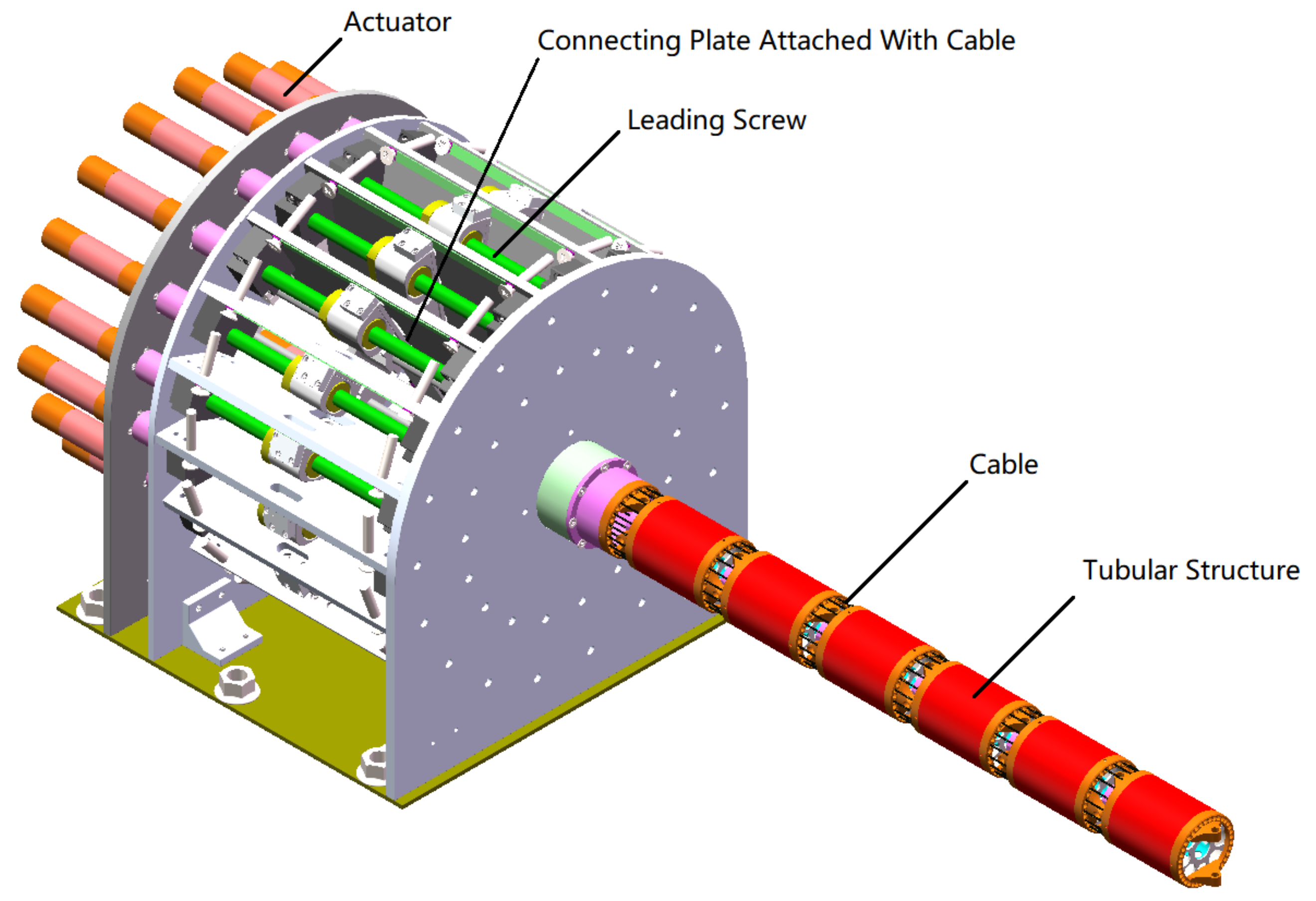
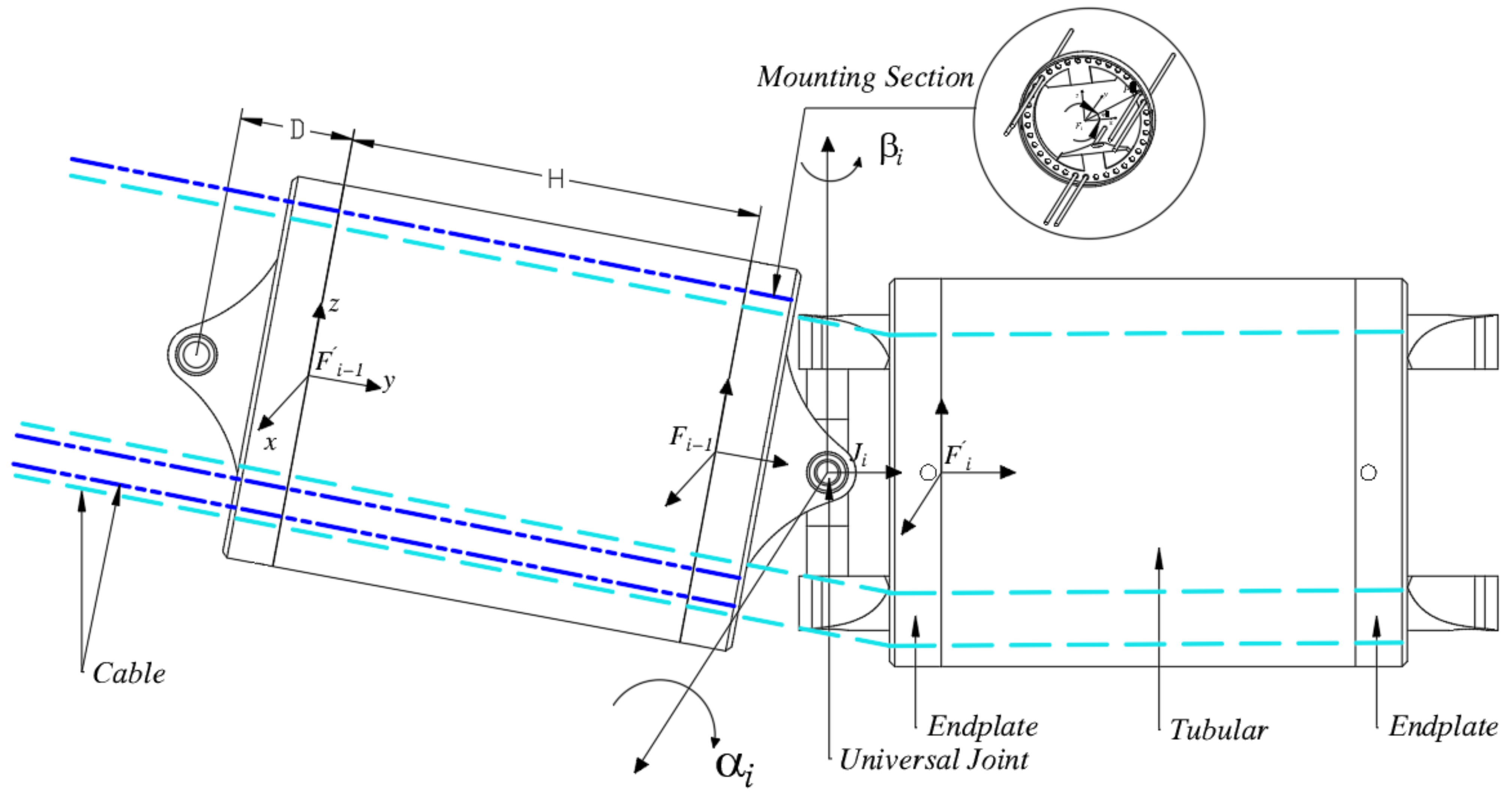
High flexibility of avoiding obstacles, good loading capacity, and easy maintenance should be taken into consideration for the structural design of snake-like manipulators to satisfy the requirement of tasks under complicated working circumstances. The proposed overall structure design of CHSM is presented in Figure 3. A separating structure is adopted in dividing the power and motion subsystem on purpose protecting the power subsystem away from harsh working circumstances but remaining the motion subsystem deploying its task normally. The motion subsystem is composed of repeated tubular structures connected to a universal joint by two fixed endplates as shown in Figure 4. Driving cables from the power subsystem get through a series of piercing holes which are uniformly distributed along the circumferential periphery in the shell of the tubular structure. Three cables are attached on the rear endplate, equally spaced at ${120}^{\circ }$ and used to drive this tubular unit meanwhile the others are maintained piercing to serving for followed tubular units respectively as shown in Figure 5. In the power subsystem, the cables are attached to the sliders which are mounted on the screw nut seat of the leading screw and drive to control the pose of each tubular by rotating upon the universal joint with 2-DOF. The motion subsystem is assembled flexibly to conveniently extend the number of joint units according to diverse task demands.

3.2. Forward Kinematics Analysis

The cable-joint kinematics can be derived from the established geometric model presented in Figure 4. The Frame $F_i$ and $F_i^{{}^{\prime }}$ are fixed on the center of where rear and proximal endplate concatenates the i-th tubular structure whose axial direction is parallel to the Y-axis. The universal joints in the geometric model can be mounted in an odd or even manner but do not influence the formulation. The cross-section for cable mounting is illustrated in Figure 5.

The main purpose of forward kinematics is to inference the end-effector’s position based on the given joint angles $[{\alpha }_i,{\beta }_i](i=1,2,...,N)$ but for CHSM the mapping transformation from unique and defined cable length $L_{i,j}(j=1,2,3)$ to the joint angles is critical and principal.

3.2.1. Coordinate Transformation Matrix between Adjacent Tubular

The pose transformation matrix of Frame $F_{i-1}$ with reference to Frame $F_i^{{}^{\prime }}$ can be formulated as:

$${}_{i-1}^{i}T=Transl(0,D,0)RotZ\left({\beta }_i\right)RotX\left({\alpha }_i\right)Transl(0,D,0)$$

(10)

where $Transl(0,D,0)$ represents the translation function with respect to Y-axis by shifting displacement D. $RotZ\left({\beta }_i\right)$ and $RotX\left({\alpha }_i\right)$ represent the rotation function regarding Z-axis and X-axis, ${\alpha }_i$ and ${\beta }_i$ denote respectively the corresponding counterclockwise rotation angle around axis. Equation (10) can be rewritten as homogeneous matrix expression:

$${}_{i-1}^{i}T=\left[\begin{array}{ccccc}& cos{\beta }_i& -cos{\alpha }_{i}sin{\beta }_i& sin{\alpha }_{i}sin{\beta }_i& -Dcos{\alpha }_{i}sin{\beta }_i\\ & sin{\beta }_i& cos{\alpha }_{i}cos{\beta }_i& -cos{\beta }_{i}sin{\alpha }_i& D+Dcos{\alpha }_{i}cos{\beta }_i\\ & 0& sin{\alpha }_i& cos{\alpha }_i& Dsin{\alpha }_i\\ & 0& 0& 0& 1\end{array}\right]$$

(11)

3.2.2. Mapping Relation between Cable and Joint

As shown in Figure 5, $P_{i,j}$ represents the mounted point of j-th $(j=1,2,3)$ cable on the rear endplate in the Frame $F_i$ and the counterclockwise angle ${\phi }_{i,j}$ can be derived as Equations (12) and (13) where M represents the total number of the holes in an endplate.

$$p_{i,j}={[R\times cos{\phi }_{i,j},0,R\times sin{\phi }_{i,j}]}^T$$

(12)

$${\phi }_{i,j}=i\times \frac{{360}^{\circ }}{M}+(j-1)\times {120}^{\circ }$$

(13)

The through hole (instead of the mounted point if this cable is used for driving subsequent tubular unit) is denoted as $p_{i,j}^{{}^{\prime }}$ in the Frame $F_i^{{}^{\prime }}$ and the Euclidean distance from $p_{i-1,j}$ to $p_{i,j}^{{}^{\prime }}$ denoted as $l_{i,j}$ which represents the cable’s length between the i-th tubular unit and the $(i+1)$-th one in the condition of considering the cable is always straight through the tube and ignoring its deformation. The total lengths of cables in k-th tubular units can be derived as Equation (15).

$$l_{i,j}=∥{}_{i-1}^{i}T\times p_{i,j}-p_{i,j}^{{}^{\prime }}∥$$

(14)

$$L_{m,j}=\sum _i^m(l_{i,j}+H)m=1,2...N$$

(15)

$L_{m,j}$ is formulated as a function $f({\phi }_{i,j},{\alpha }_i,{\beta }_i)$ once all the cables’ lengths are given, each joint angle $[{\alpha }_i,{\beta }_i]$ will be derived uniquely and definitely with respect to Equations (10)–(15).

3.2.3. End-Effector Pose Expression

The end-effector is fixed on the N-th tubular unit and the coordinate transformation matrix is denoted as ${}_N^{E}T$ similarly to ${}_{i-1}^{i}T$. The coordinate transformation matrix from base to the end-effector can be derived as Equation (16) where the $F_0$ represents the global coordinate Frame.

$${}_0^{E}T=\prod _{i=1}^N{(}_{i-1}^{i}T\times Trans(0,H,0)){\times }_N^{E}T$$

(16)

The pose of end-effector can be achieved from Equations (10)–(16) due to the forward kinematics model is stated explicitly from cable space to the working space based on the equations described above. The camera for visual tracking undertakes the obligation of the end-effector in the scenario of this article.

3.3. Inverse Kinematics

In general, inverse kinematics is much more complicated than forward kinematics especially for CHSM due to its high level of redundant DOF which means numerous analytical solutions. Otherwise, the numerical method suffers severe penalty from solving the pseudo-inverse of the Jacobian matrix which costs increasing rapidly computation time. Under these circumstances, an efficient, simplified, and accessible solution could be taken advantage instead of the numerical method.

Two assumptions are introduced to simplify the joints’ motion. First, the last tubular unit keeps horizontal direction paralleling to the Y-axis of the world coordinate system. This restriction improves stability for the visual sampling and keeps away from image distortion. Furthermore, the N-th joint angle $[{\alpha }_N,{\beta }_N]$ could be easily obtained from $[{\alpha }_N,{\beta }_N]+{\sum }_{i=0}^{N-1}[{\alpha }_i,{\beta }_i]=0$ if the other ones are definite. Second, adjust each joint as slightly as possible and primarily use the last couple of joints during moving the end-effector to the desired position. That means if the desired position is contained in the working space of the last three tubular units, the last three joints should be adjusted, and the others should keep remaining unchanged. When the desired position is beyond working space, a requirement of adding some new left-neighbor tubular unit arises. Under this condition, we simplify the model into a Three-Connecting-Rod Mechanism by forcing the middle tubular units to form a straight line which means their joint angles are set to zero.

In the simple model, the tubular units and universal joints are substituted by lines (with a length of $L=H+2D$) and dots respectively where $A_{Nd}$ represents the N-th joint’s position. The subscripts d and o denote the desired position and the initial position. After the tracking target’s moving trajectory is captured by the tracking component, $A_{Nd}$ is definite and the number m of demanding joints to be adjusted can be inferred according to Equation (17). Equation (17) means the desired position is beyond the working space of the last $N-m-1$ joints but is contained in the working space of the last $N-m$ ones.

$$\left\{\begin{array}{c}∥A_{Nd}-A_{(m+1)o}∥ \ge (N-m-1)\times L\\ ∥A_{Nd}-A_{mo}∥ \le (N-m)\times L\end{array}\right.$$

(17)

Based on the simplified Three-Connecting-Rod Mechanism the $A_{md}$, $A_{(m+1)d}$ and $A_{Nd}$ satisfies Equation (18).

$$\left\{\begin{array}{c}∥A_{Nd}-A_{(m+1)d}∥ =(N-m-1)\times L\\ ∥A_{(m+1)d}-A_{md}∥=L\end{array}\right.$$

(18)

$A_{(m+1)d}$ is located on an intersecting circle between a sphere (center at $A_{md}$, radius of L) and another (center at $A_{Nd}$, radius of $(N-m-1)L$). Following the second assumption the $A_{(m+1)d}$ is accessible and the other $A_{id},i=m,m+2,...,N-1$ could be inferenced via the coordinate transformation introduced earlier.

3.4. Control Method

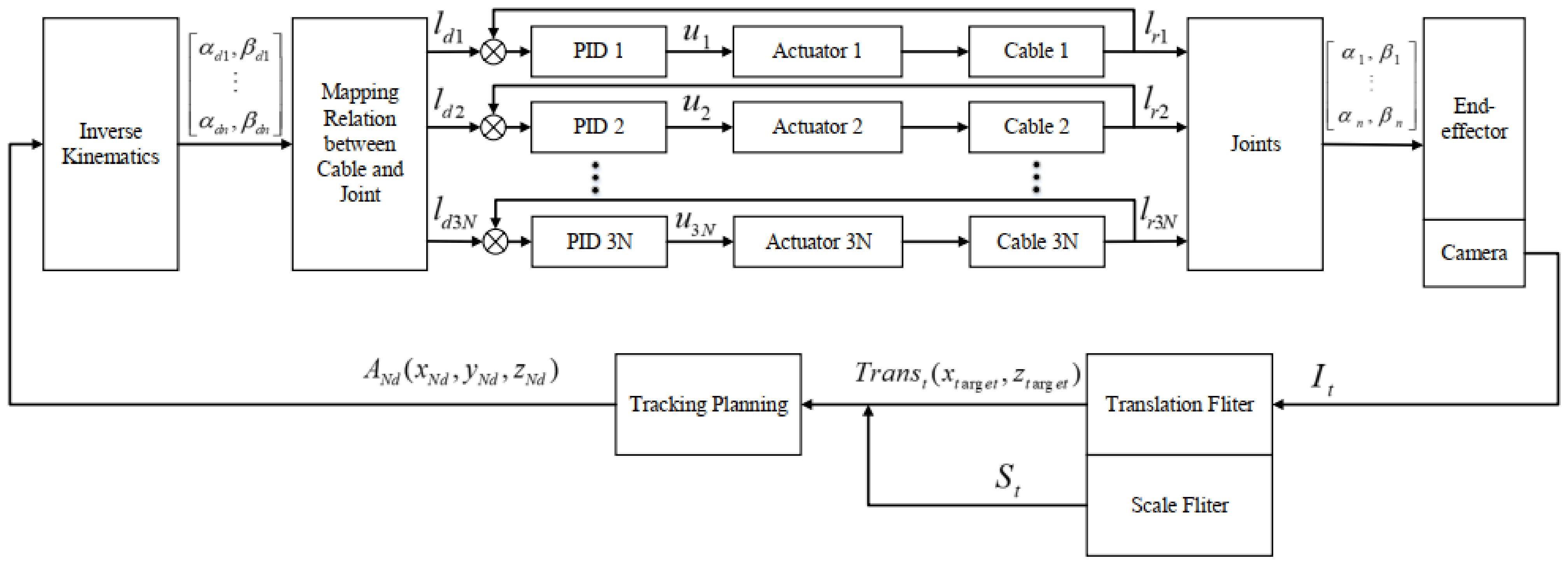
Based on the kinematics discussed previously, a control scheme of CHSM is shown in Figure 6. For the object tracking task, the end-effector is trying to follow the object’s moving trajectory and keep a constant distance from the target. The tracking component is applied to infer the target’s position in the working space according to that in the pixel space by multiplying the inverse instinct matrix of the camera and then calculate the desired end-effector’s pose $A_{Nd}(x_{Nd},y_{Nd},z_{Nd})$. The desired cable’s length $l_{di}(i=1,2,...,3N)$ are calculated from Equations (11)–(15) with desired joint angle $[{\alpha }_{di},{\beta }_{di}](i=1,2,...,N)$ obtained from the inverse kinematics with $A_{Nd}$. The linear magnetic encoder mounted on the actuator measures each practical cable length $l_{ri}(i=1,2,...,3N)$ as inputs for the closed-loop PID controller which is designed as follows:

$$u=K_P(l_d-l_r)+K_I{\int }_0^t(l_d-l_r)d\tau +K_D({\dot{l}}_d-{\dot{l}}_r)$$

(19)

where $K_P,K_I,K_D$ are PID parameters and the output has a linear proportional relation with the cable’s stretching speed.

4. Experiment and Validation

In this section, an experiment is implemented to validate the moving and controlling performances of CHSM based on the introduced visual tracking.

The prototype platform used for the experiment is shown in Figure 7. The primary parameters are illustrated in

Table 1. Some parameters selected in the experiment.

Parameters	Description	Values
$\lambda$	Regularization parameter of ridge regression	0.01
$\eta$	Learning rate for updating correlation filter	0.025
N	Number of tubular units	5
D	Distance from endplate to universal joint	12 mm
R	Radius of tubular structure	33.8 mm
H	Length of tubular structure	106 mm

. Moreover, the PID parameters $K_P,K_I,K_D$ are selected as $K_P=5,K_I=2,K_D=0.05$ in a comprehensive consideration both for rapid response and stability of each actuator. The displacement signal of cable collected by Quanser QUARC software from the linear magnetic encoder to PID controller and the reverse controlling signal are all aggregated and passed via the real-time platform Simulink/Matlab with a sampling frequency at 100 HZ. The visual servo feedback referring signal is captured by the camera (attached on the end tubular structural unit) which is working in BGR color space and 30 HZ refresh frequency. HOG features perform better and are adopted in the next experiments.

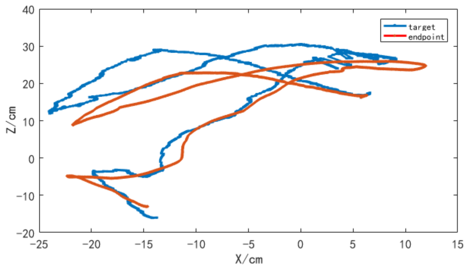
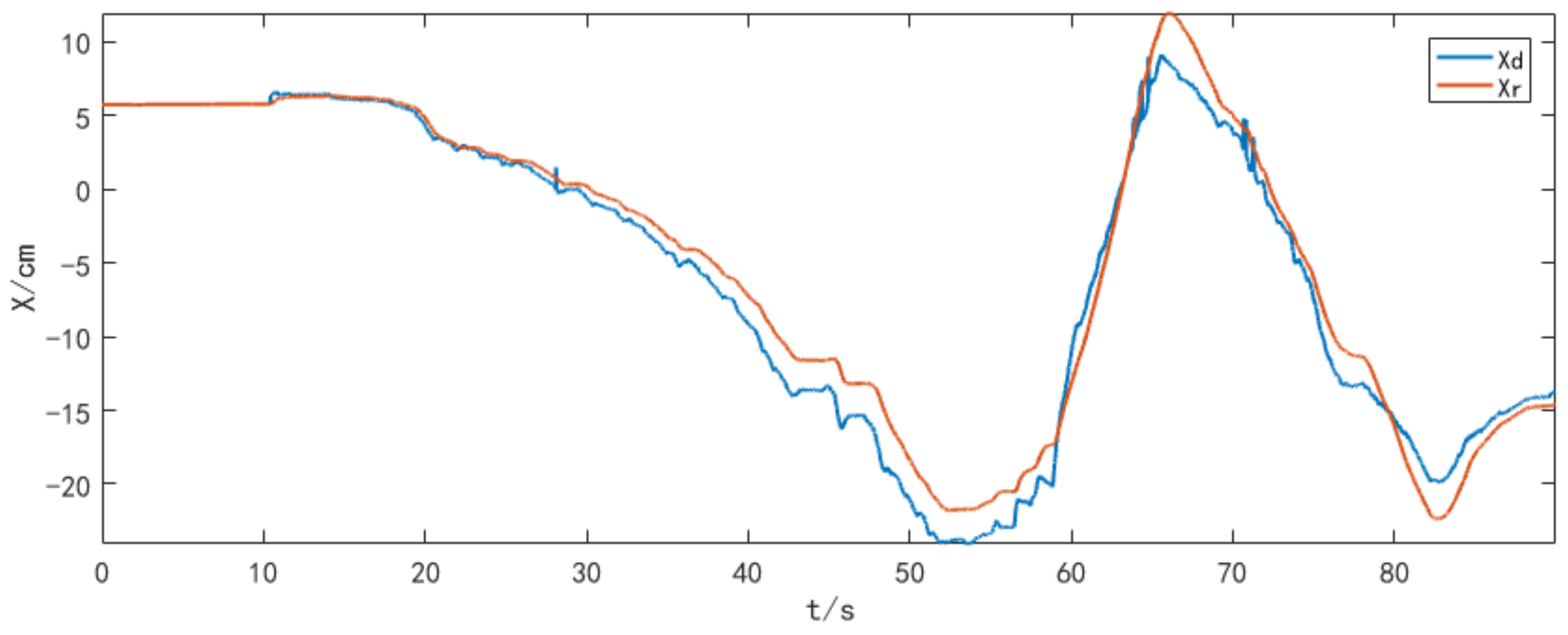
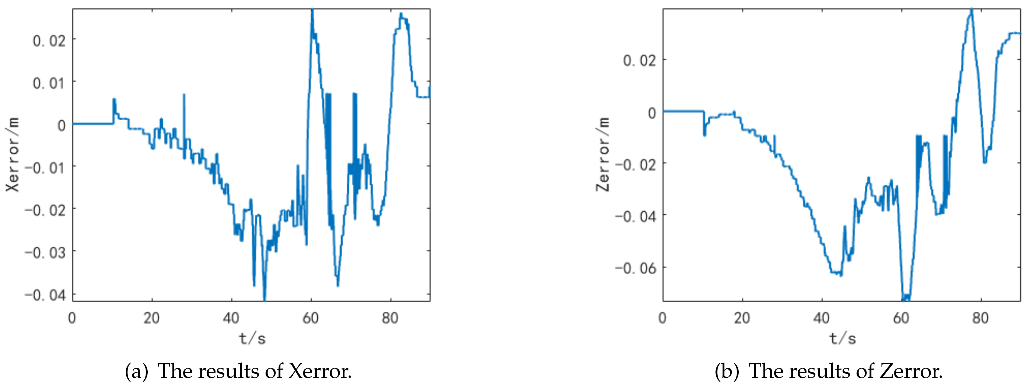
The experimental results of tracking target are shown in Figure 8, Figure 9, Figure 10 and Figure 11, where the target is moving towards a random direction with a slowly increasing velocity earlier and then reduced to a normal level later. The tracking component can accurately capture the target in the visual field and driving the CHSM to adjust its pose (according to the Kinematics Equations (11)–(18)) to focus on the target, which means the target always appears at the center of the camera’s perceived screen in every frame. In that case, the moving trajectory of CHSM’s endpoint should be identical to the target as closely as possible. The CHSM’s moving in the Y-axis is limited to a narrow range due to the scale adaptation of the tracking component. Figure 9 and Figure 10 show the experimental result of the X-axis and Z-axis, respectively.

The subscript labels $d,r$ represent the target and the CHSM’s endpoint respectively and have the same meaning in the Figure 11.

CHSM has a good tracking performance with the target except for a little delay. The absolute value of error has the same variation tendency as the target’s moving speed which may be caused by the limited sampling scope of the tracking component.

Figure 12 shows the recorded perspective from the camera when the target is moving dragged by a rope and four frames are selected as representatives. The target is detected and highlighted by a green bounding box which is nearly located in the center of the frames. When the target moves, the tracking component detects the target’s new position and guides the CHSM to focus on the target so that the bounding box looks such as rooting on the center. The bounding box’s deviation from the center has the same tendency as the error (shown in Figure 11).

5. Conclusion and Future Work

In this paper, we introduce a cable-driven hyper-redundant snake-like manipulator (CHSM), then build up a rigorous forward kinematics model base on coordinate transformation and a simplified inverse kinematics model via geometry relationships which has a low time-consuming for real-time control. The correlation filter technique is introduced to get on well with the tracking task, optimized for the adaptive scale variation, and improved on the robustness under the visual servo. The experimental result shows that CHSM has a good trajectory tracking performance and is endowed with some intelligence by the visual tracking technique. This work brings an advanced computer vision technique into the cable-driven snake-like manipulator to form an intelligent scheme. This scheme can be conveniently expanded for more advanced computer vision techniques involved on comprehensive tasks.

The future work will be carried out as follows. The weight of one tubular unit is a little beyond our expectation which restricts the extension for several units and impacts loading capacity. We have considered two aspects for optimizing it, reducing the radius of the tubular structure or finding an advanced composite material (e.g., carbon fiber reinforced polymer, etc.) instead of steel. The study of this paper is launched on the assumption that the end-effector is restricted to keeping horizontal orientation so that the camera’s field of view is limited to some degree. In future work, this restriction will be relieved, and the end-effector can orientate toward any direction to assure that the manipulator can respond with minimal translation or rotation which is critical under the high-speed tracking circumstance. Meanwhile, the inverse kinematics and control loop should be redesigned.