Considerations about Parameters Estimation into a Minimum Variance Control System

Abstract

The starting point to design a minimum variance control law consists in identifying a linearized mathematical model (valid around an operating point) of a nonlinear process, respectively the on-line estimation of the parameters of this model. This paper presents a comparative study regarding the estimation of these parameters for the case when the process operates in open-loop, respectively the process is integrated into a closed-loop system specific to a minimum variance control. The comparison is made both analytically (for the general case) and through a validation study (by simulation) particularized for the case of an induction generator integrated into a wind energy conversion system. The main contribution of this paper consists in proving the fact that, in closed-loop (under the constraints imposed by the control law), the process parameters estimates differ from the real ones identified in open-loop (in free operating mode, without constraints). In addition, as a novelty, the paper demonstrates that, in steady-state, the process gain estimates are identical, both in closed-loop and open-loop, even though they are calculated based on different estimates of these linear model parameters. Thus, based on parameters estimates in closed-loop, the parameter estimator rather allows the estimation of the real process gain, although it does not accurately estimate the real values of the linearized model parameters (correctly estimated only in open-loop).

1. Introduction

Based on adaptive feature, the minimum variance control systems represent viable solutions for nonlinear process control, for which classical control solutions are difficult to implement due to nonlinearities [1,2,3,4,5,6]. This adaptive feature of such control system is assured by the integration in its structure of an on-line parameters estimator for a linearized model, which describes the nonlinear process functionality around a functioning point. Thus, for the design of a minimum variance control law, the starting point is the identification of a linearized model for the considered process. In the present work, the recursive least squares (RLS) estimator was considered.

The control law, designed for an operating point, is obtained by minimizing a criterion function that contains a sum of two quadratic terms (see Equation (1), where E is an expectation operator). The first quadratic term assures the minimization of the controlled output variance, respectively the second term (weighted by a control penalty factor) allows a minimization of the control variance, absolutely necessary in order to obtain physically achievable control values and implicit stability of the control system [7,8,9]. The technical literature states that in practice the control penalty factor is usually set in the range $\rho =0.0001\dots 0.1$, ensuring a proper control variance penalization [2,5,8].

$$J=E\left\{{\left[\mathrm{output} \mathrm{variance}\right]}^2+\rho {\left[\mathrm{control} \mathrm{variance}\right]}^2\right\}$$

(1)

Although designed based on a linearized model, the real-time estimation and the continuous tracking of the estimates changes leads to a nonlinear control law. In the present paper, it will be proved analytically and validated through a numerical simulation (for a particular chosen case) that, in the closed-loop (due to the constraints imposed by the minimum variance control law), the linear model parameters estimates are not identical with the real ones estimated when the process operates in open-loop. In spite of this fact, in the steady-state (and based on different estimates for the open-loop, respectively the closed-loop regime), the process gain computation for both cases leads to similar values. In other words, in the closed-loop, the parameter estimator allows the computation of exact values of the steady-state process gain and not of the real parameters estimates (taking into account that the real values are the ones obtained in open-loop).

The demonstration of the above mentioned was performed analytically and validated through simulations for the case of an induction generator integrated into a wind energy conversion system (a strong nonlinear process). Even if the complete functionality of an induction generator is described by a seventh order nonlinear model (the classical Park’s equations [10,11]), the technical literature shows that its functionality can be approximated by a fourth order linearized model, accurately enough around an operating point [11,12,13]. This simplified linearized model is used only for the design of the minimum variance control law and, obviously, the accurate seventh order nonlinear model is used to simulate the process. For the tuning of the minimum variance control system (an issue that is not subject of this paper, but is well described by technical literature [6,8,14]), appropriate values have been set for the control penalty factor ($\rho$) and for the estimator’s forgetting factor (λ). In addition, the plant will be disturbed by a stochastic noise of zero mean and σ² = 0.01 variance (ensuring the numerical stability of the RLS estimator) [15,16,17,18,19]. The main objective of the control system is to maintain a constant terminal voltage in two operating regimes, under the action of external disturbances such as: mechanical torque variation (due to wind speed changes), respectively load/unload disturbance (by connecting/disconnecting electrical consumers at induction generator terminals).

Many papers are focused on control performances and less on parameters estimation, which is a vital part of a minimum variance control system [2,5,8]. Precisely this punctual issue of parameters estimation is addressed in this paper. As the manuscript title states, the main goal is to perform a comparative analysis regarding the process parameters estimates (both in open and closed-loop) and not to analyze the control system performances (topic presented by many works, including those of the authors [8,9,14,20]). As will be shown below, such an analysis of the estimation process, performed in open-loop or closed-loop operating conditions, leads to some interesting conclusions regarding the process parameters estimates, respectively the process gain estimate. All these findings are valid only for the identification and control of a nonlinear process (whose limited functionality around an operating point can obviously be described by a linearized model).

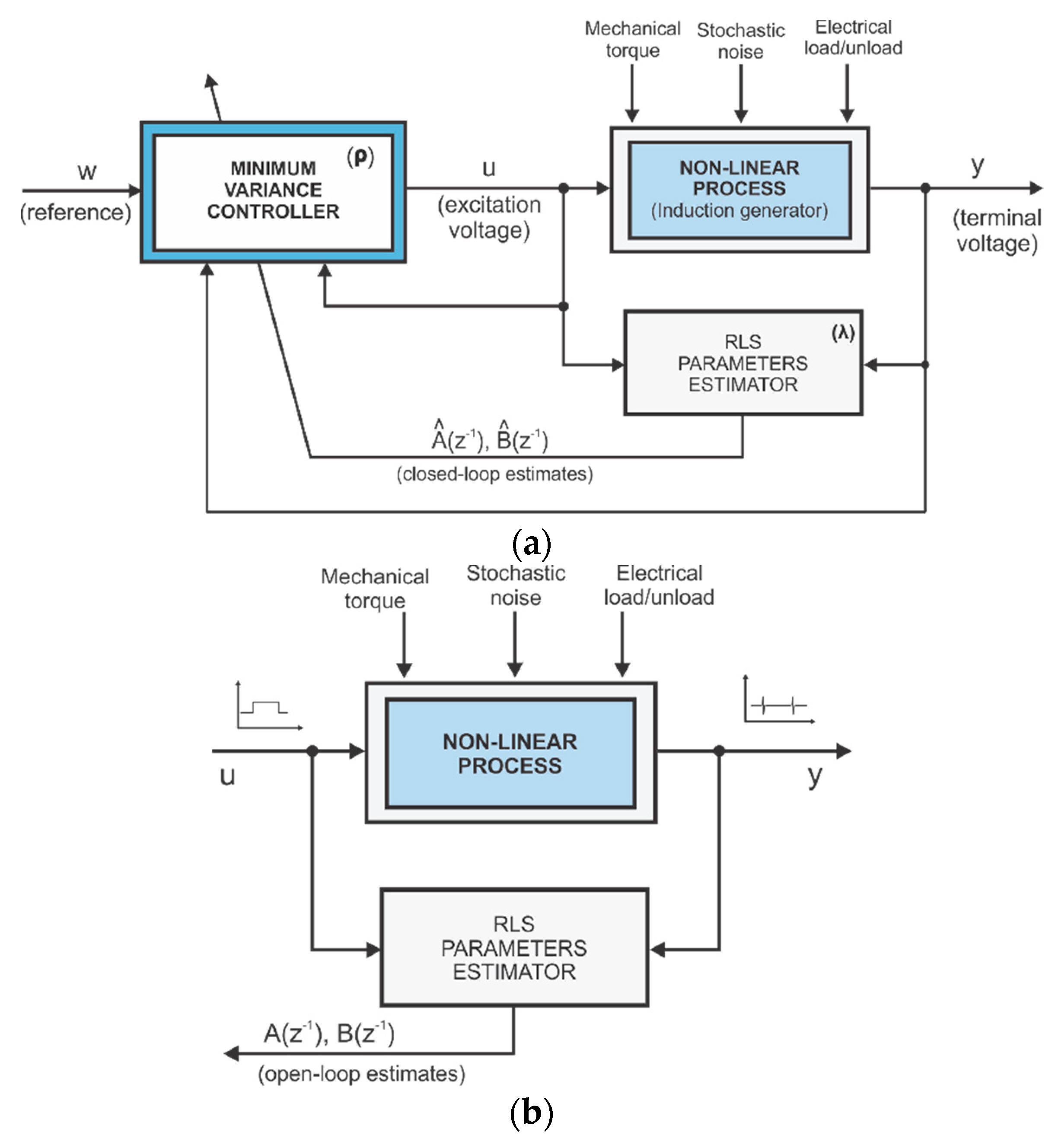
2. Analytical Demonstration Based on Minimum Variance Control Law Design

The general structure of a minimum variance control system (particularized for the considered process-an induction generator integrated into a wind energy conversion system), is depicted in Figure 1a. In addition, the nonlinear process operating in open-loop is illustrated in Figure 1b.

As already mentioned, the starting point of a minimum variance control law design is a linear model described by a discrete difference equation (Equation (2)):

$$A\left(z^{-1}\right)y_t=z^{-1}B\left(z^{-1}\right)u_t$$

(2)

where: $A\left(z^{-1}\right)$ and $B\left(z^{-1}\right)$ are polynomials in $z^{-1}$ shift operator, $y_t$-process output at discrete time t (terminal voltage for the considered process), $u_t$-process input (excitation voltage), $z^{-1}$-shift operator (with one sampling time, therefore $y_t=z^{-1}{y}_{t+1}, y_{t-1}=z^{-1}{y}_t$, and so on).

This discrete linear model (Equation (2)) is valid around an operating point, for a proper set of parameters values. Another operating point means another set of parameters values.

The control law design involves minimizing a criterion function described by Equation (3) [2,8,9,20]:

$$J=E\left\{{\left[y_{t+1}-w_t\right]}^2+\rho {\left[u_t-u_t^{*}\right]}^2\right\}$$

(3)

where, in the context of a control system: $y_{t+1}$-controlled output at discrete time t + 1 (next sampling time); $u_t$-controller output and $u_t^{*}$ –steady state controller output; $w_t$-set point (reference), ρ-control penalty factor (properly set); E{.}-mean operator (expectation).

Considering a steady state regime, therefore $z^{-1}=1$ and $u_t^{*}=\frac{\widehat{A}\left(1\right)}{\widehat{B}\left(1\right)}{y}_t$ (through ^ being noted the estimates of polynomials from Equation (2)), by minimizing the criterion function (Equation (3)) and solving the equation $\frac{dJ}{d{u}_t}=0$, the following control law is obtained [9,13,20]:

$$u_t=\frac{-\mathrm{z}\left[1-\widehat{A}\left(z^{-1}\right)\right]}{\widehat{B}\left(z^{-1}\right)+\rho }{y}_t+\frac{1+\rho \frac{\widehat{A}\left(1\right)}{\widehat{B}\left(1\right)}}{\widehat{B}\left(z^{-1}\right)+\rho }{w}_t$$

(4)

It should be noted that $\widehat{A}\left(z^{-1}\right)$ and $\widehat{B}\left(z^{-1}\right)$ are the estimated polynomials (in closed-loop) which approximates the real polynomials $A\left(z^{-1}\right)$ and $B\left(z^{-1}\right)$ (identified in open-loop).

Based on linear model described by Equation (2), $y_t=z^{-1}\frac{B\left(z^{-1}\right)}{A\left(z^{-1}\right)}{u}_t$ and in the steady state ($z^{-1}=1$), under the control system constraints, the reference and the controlled output are equal: $w_t=y_t$. Taking into account those mentioned and substituting $w_t$ and $y_t$ in Equation (4), it results:

$$u_t=\frac{-\left[1-\widehat{A}\left(1\right)\right]+1+\rho \frac{\widehat{A}\left(1\right)}{\widehat{B}\left(1\right)}}{\widehat{B}\left(1\right)+\rho }\frac{B\left(1\right)}{A\left(1\right)}{u}_t$$

(5)

By simplifying with $u_t$, Equation (5) becomes:

$$A\left(1\right)\widehat{B}\left(1\right)+\rho A\left(1\right)=\widehat{A}\left(1\right)B\left(1\right)+\rho \frac{\widehat{A}\left(1\right)}{\widehat{B}\left(1\right)}B\left(1\right)$$

(6)

Multiplying Equation (6) with $\widehat{B}\left(1\right)$ and grouping on the right member the terms depending on $\rho ,$ it is obtained:

$$\widehat{B}\left(1\right)\underset{0}{\underbrace{\left[A\left(1\right)\widehat{B}\left(1\right)-\widehat{A}\left(1\right)B\left(1\right)\right]}}=-\rho \underset{0}{\underbrace{[A\left(1\right)\widehat{B}\left(1\right)-\widehat{A}\left(1\right)B\left(1\right)}}]$$

(7)

The equality Equation (7) (valid in steady-state) can be fulfilled only if both right member and left member are zero, leading to the following equality relation (practically the same, fulfilled by both members):

$$\frac{\widehat{B}\left(1\right)}{\widehat{A}\left(1\right)}=\frac{B\left(1\right)}{A\left(1\right)}$$

(8)

Supposing that $A\left(1\right)\widehat{B}\left(1\right)-\widehat{A}\left(1\right)B\left(1\right)\ne 0$ and simplifying the equality (7) with $A\left(1\right)\widehat{B}\left(1\right)-\widehat{A}\left(1\right)B\left(1\right)$, for the fulfillment of this equality would result: $\widehat{B}\left(1\right)=-\rho$. However, the control penalty factor $\rho$ is a chosen constant and $\widehat{B}\left(1\right)$ is a variable estimate (which changes with the operating point), so the condition $\widehat{B}\left(1\right)=-\rho$ cannot be met. Thus, the only solution for achieving equality described by Equation (7) remains the fulfillment of condition $A\left(1\right)\widehat{B}\left(1\right)-\widehat{A}\left(1\right)B\left(1\right)=0$ (in both members).

Equation (8) does not necessarily involve strictly equalities of the fractions numerators, (respectively denominators), but only the equality of these ratios. These fractions are practical gain factors of the process.

By noting:

$$\{\begin{array}{c}{k}_{gain}=\frac{B\left(1\right)}{A\left(1\right)} \\ {\widehat{k}}_{gain}=\frac{\widehat{B}\left(1\right)}{\widehat{A}\left(1\right)}\end{array}$$

(9)

where: $k_{gain}$-the open-loop process gain factor and ${\widehat{k}}_{gain}$-the closed-loop process gain factor, based on equality described by Equation (8) it results:

$$k_{gain}={\widehat{k}}_{gain}$$

(10)

As a conclusion, in steady-state closed-loop regime, although parameters estimates may differ from those in the open-loop (so, $\widehat{A}\left(1\right)\ne A\left(1\right)$ and $\widehat{B}\left(1\right)\ne B\left(1\right)$), the process gain estimates are similar both in open-loop and closed-loop (see Equation (10)). Therefore, for a proper operating of the control system, it’s not even necessary an accurate estimation of the real parameters of the process linearized model, but only an accurate estimation of the process gain.

3. Case Studies for Validation

For the validation of the analytical demonstration presented for the general case in previous chapter, an induction generator (a strong nonlinear process) integrated into a wind energy conversion system is considered as controlled plant. As already mentioned, the goal of the minimum variance control system is to maintain a constant terminal voltage, rejecting the external disturbances such as mechanical torque variation (due to wind speed variation), respectively load/unload (due to connecting/disconnecting electrical consumers at terminals). For the modeling and simulation of the induction generator, a nonlinear seventh order model (the d-q axis model) was used, fully describing its functionality [11,12,20,21]. The complete model of the wind energy conversion system is presented in the already published paper [13] of authors. It must be emphasized, once again, that the identified linearized model of the fourth order, describing the induction generator behavior around an operating point, was used only for the design of the control law [10,12,20]. Thus, for the linear model described by Equation (2), the component polynomials are detailed in Equation (11):

$$\begin{array}{c}A\left(z^{-1}\right)=a_4{z}^{-4}+a_3{z}^{-3}+a_2{z}^{-2}+a_1{z}^{-1}+1\\ B\left(z^{-1}\right)=b_3{z}^{-3}+b_2{z}^{-2}+b_1{z}^{-1}+b_0\end{array}$$

(11)

Furthermore, and obviously, in steady state regime ($z^{-1}=1$), the computed gain (based on parameters estimates) is:

$$k_{gain}=\frac{b_3+b_2+b_1+b_0}{a_4+a_3+a_2+a_1+1}$$

(12)

The minimum variance control system is considered disturbed by a zero-mean stochastic noise with variance σ² = 0.01 and the control penalty factor is set to the value $\rho =0.01$. In addition, for the recursive least squares (RLS) estimator integrated into the control system, the forgetting factor is set to the value $\lambda =0.995$. The values set of the two tuning parameters ($\rho ,\lambda$) of the control system assures good control performances [9,13,20].

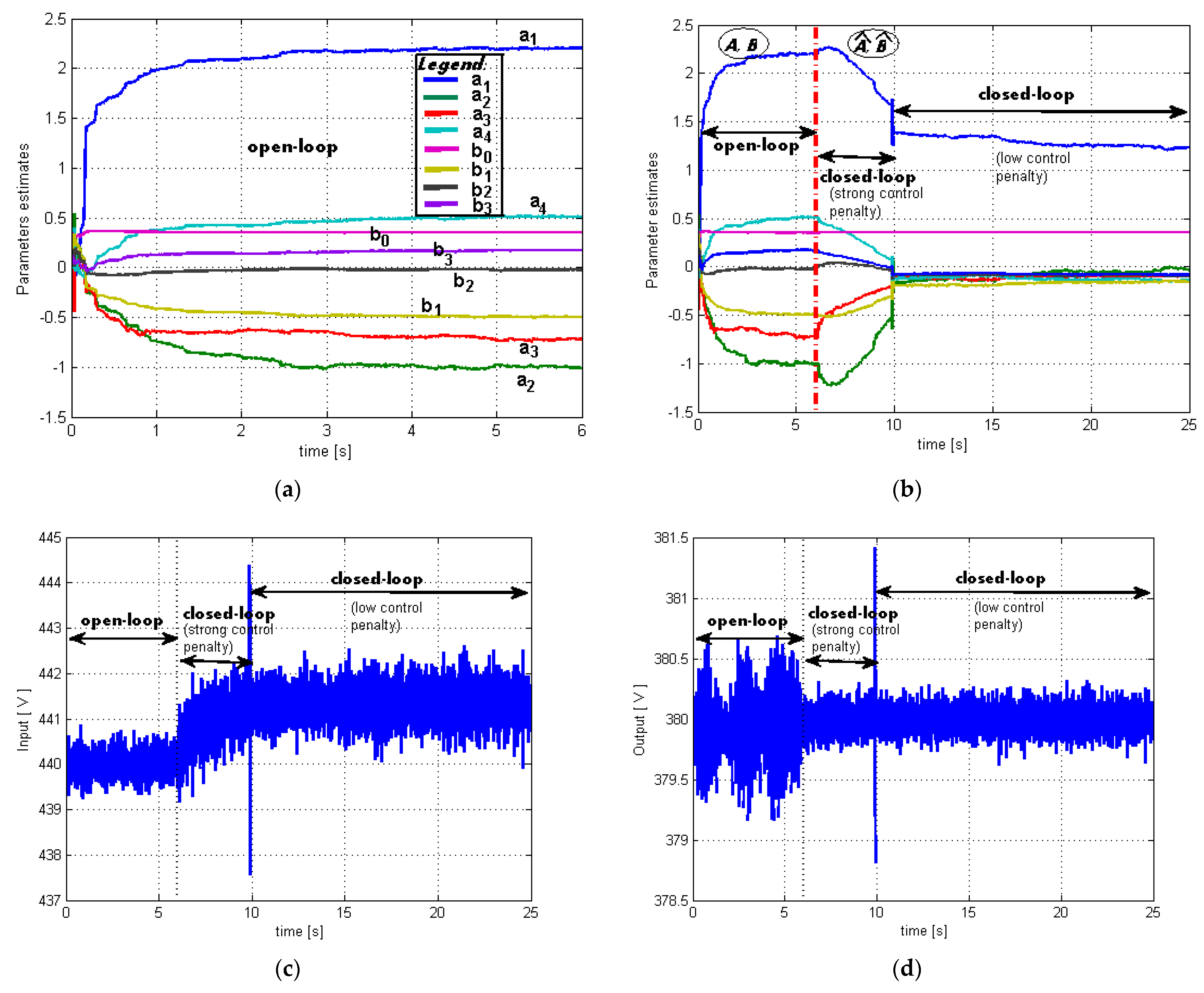
3.1. Case 1. Initialization of the Minimum Variance Control System

The starting of a minimum variance control system is a complex process, requiring several steps [8,9].

The first step is to start the open-loop process, for computation and initialization of the linearized model parameters. The considered operating point is defined by the following conditions: step input excitation voltage: 440 V, zero initial values of the estimates, process input disturbed by a zero-mean stochastic noise and variance σ² = 0.01. In this case, the estimates of the model parameters are presented in Figure 2a (practically a zoom of the initial time interval ($t=\left[0 6\right] s)$ from Figure 2b presenting the estimates for the complete procedure of starting and initializing the control system, as will be shown below). The same colors used in Figure 2a (see the figure legend) to represent the parameters estimates of polynomials described by Equation (11) are used for all next case studies which will present parameters estimates ($a_{1\dots 4},b_{0\dots 3}$ in open-loop and ${\widehat{\mathrm{a}}}_{1\dots 4},{\widehat{b}}_{0\dots 3}$ in closed-loop).

In the second step, the loop is closed (performing a synchronization between the controller and the plant) and an initial tuning of the control penalty factor to a high value $\rho =0.1$ is performed to ensure the control system stability and an efficient control penalization [8,9]. The last step requires a decrease of the control penalty ($\rho =0.01$), allowing a higher control and much better performances [7,8,9,22,23,24,25,26]. All these operating stages are highlighted and can be observed in Figure 2b–d. Figure 2c presents the controller output (the control loop is closed after time moment t = 6 s and the control penalty factor is changed at time moment t = 10 s from $\rho =0.1$ to $\rho =0.01$). Figure 2d shows the controlled output. It can be noticed that the closing of the control loop leads to a decrease of the controlled output variance after time moment t = 6 s, according to the control goal.

The purpose of this case study is to demonstrate that, into a well-established operating point, by closing the control loop, the parameter estimates of the linearized model are different from those obtained in the open-loop. Thus, by analyzing the estimates presented in Figure 2b, different evolutions of the estimates for each stage can be observed. As already stated, the initial estimates until the moment t = 6 s, are those from Figure 2a (open-loop). Immediately after closing the loop (at time moment t = 6 s), the time evolution of the estimates changes under the action of the constraints imposed by the control system. Moreover, without changing the operating point of the controlled process, just a simple retuning of the minimum variance controller (by decreasing the control penalty factor at time t = 10 s) affects the parameters estimates (see the same Figure 2b).

The resulted conclusion is that the constraints imposed by the control law in closed-loop affect the estimates.

The following studies present disturbed regimes and perform an analysis regarding the parameters estimates, respectively, the process gain in the two considered operating cases: open-loop and closed-loop.

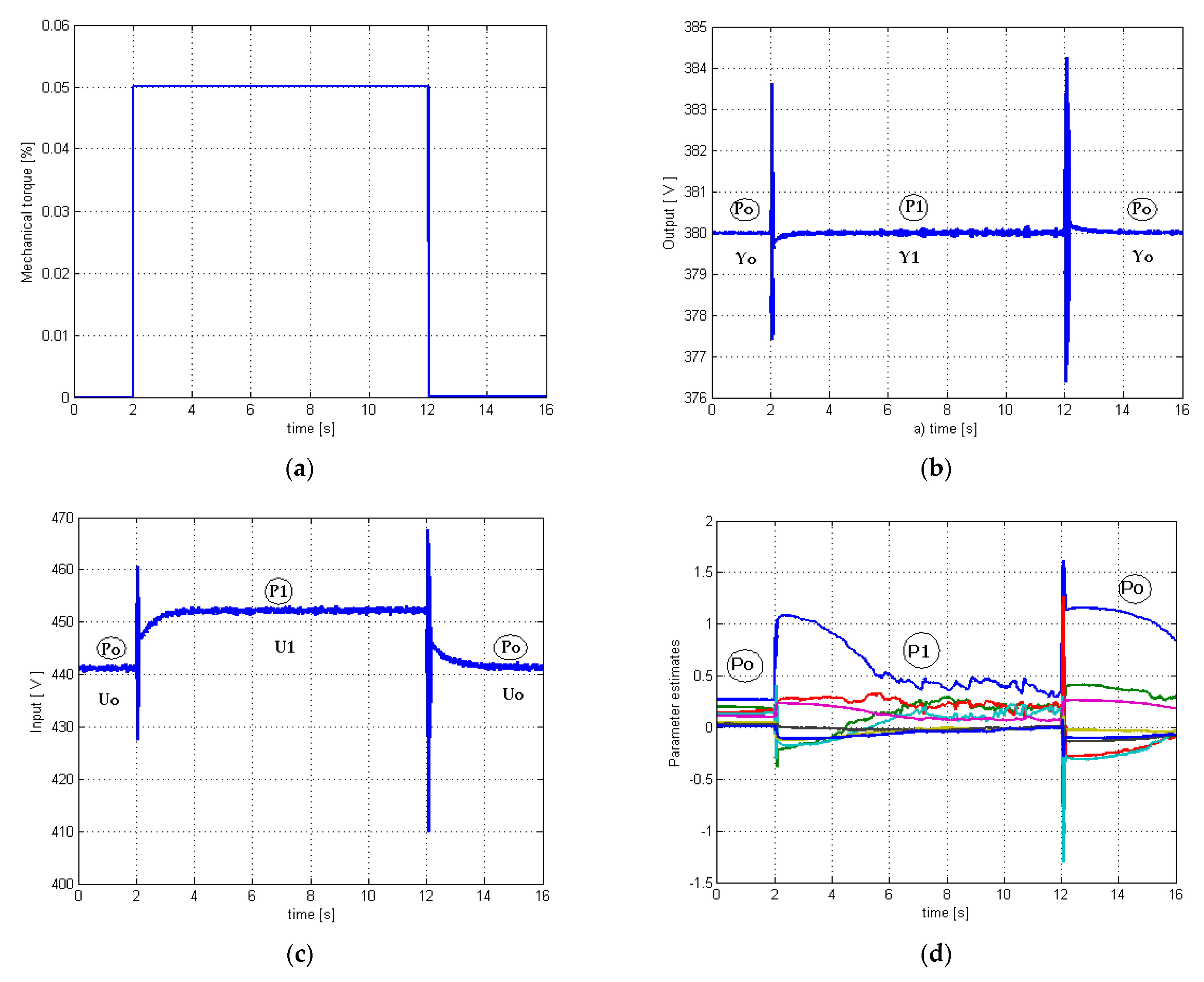
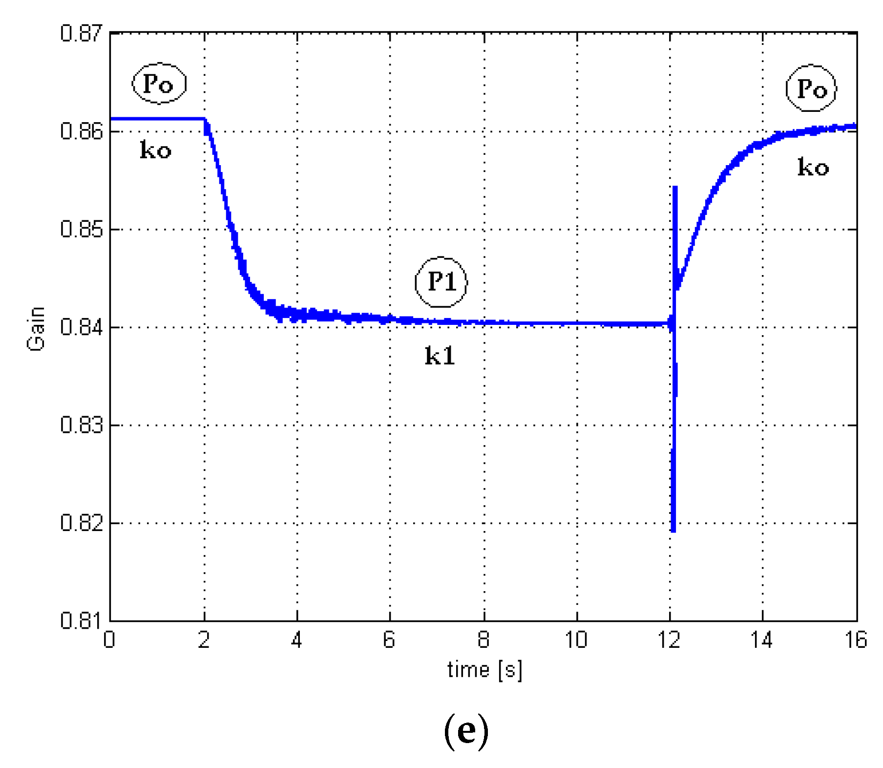
3.2. Case 2. Mechanical Torque Variation

In the following case studies, the process is considered disturbed (both in open and closed-loop) by a successively variation of the mechanical torque at time moments t = 2 s and t = 12 s (Figure 3a).

Case 2a: First, the closed-loop case is analyzed. Figure 3b,c show the terminal voltage (the controlled output), respectively, as well as the excitation voltage (the controller output) (small overshoots, small settling times, good control penalization). In Figure 3d is presented the time evolution of the parameter estimates and, based on them, in Figure 3e is computed and presented the closed-loop process gain estimate. By P₀ and P₁ are noted the steady-state operating points and very good performances can be noticed of the controlled process (induction generator): P₀-before time moment t = 2 s, P₁-between time moments t = 2 s and t = 12 s, and again P₀-after time moment t = 12 s.

Regarding these operating points, Figure 4 presents the operational characteristics of the induction generator disturbed by mechanical torque variations. The initial operating point is ${\mathrm{P}}_0$ (placed on the curve corresponding to a mechanical torque $M_0$). In the closed loop, under the action of the control system that maintains constant terminal voltage ($y_0$) and under the action of a disturbance produced by the variation of the mechanical torque ($M_1=M_0+\Delta M$), the operating point horizontally slides on another operating curve (corresponding to the new mechanical torque $M_1$) and moves to position ${\mathrm{P}}_1$. In Figure 3e can be noticed the steady-state values $k_0$ and $k_1$ of the process gain corresponding to the two closed-loop operating points ${\mathrm{P}}_0\left(u_{0, }{y}_0,M_0\right)$ and ${\mathrm{P}}_1\left(u_{1, }{y}_0,M_1\right)$ depicted in Figure 4. This representation of the induction generator operational characteristics is necessary to explain the setting of similar operating conditions in both the open and the closed-loop.

Case 2b: The next case study considers the open-loop process (perturbed by the same stochastic noise). The first temptation is to consider (as process input) a constant excitation voltage $U=U_0$, respectively at time moments t = 2 s and t = 12 s, a change of the mechanical torque ($\Delta M=\pm 5\%$, as in the previous closed-loop case). However, these operating conditions lead the process from the initial operating point P₀ to the operating point ${\mathrm{P}}_2\left(u_{0, }{y}_1,M_1\right)$ (other than the desired point P₁), and respectively back to P₀ (see Figure 4). For the process transition between these operating points P₀-> P₂-> P₀, the parameters estimates are presented in Figure 5a and, based on them, the calculated gain is presented in Figure 5b. Comparing the results from Figure 3d and Figure 5a), a different variation of the parameters estimates can be observed. However, more important is the fact that, by comparing the results from Figure 3e and Figure 5b, it can be noticed the value inconsistency regarding the median time zone (the time interval between t = 2 s and t = 12 s) of the computed gain factor in closed-loop ($k_1\approx 0.84$), respectively, in open-loop ($k_2\approx 0.86$). This value discrepancy can be explained by the fact that the open loop operating conditions took into account only the disturbances action (mechanical torque variation), which lead the process to the operating point ${\mathrm{P}}_2$ and not to the desired target point ${\mathrm{P}}_1$ (see Figure 4). Obviously, for different operating points, the gain values are different.

Therefore, it is necessary to correct the open-loop operating conditions by considering an appropriate variation of the process input (excitation voltage: $u_1=u_0+\Delta u$), which maintains a constant terminal voltage ($y_0$) and thus the operating point follows the desired transition P₀-> P₁-> P₀ (see Figure 4). In these new conditions and for the adequate operating point transition P₀-> P₁-> P₀, Figure 6a shows the open-loop process parameters estimates, respectively Figure 6b shows the process gain computed based on them.

Comparing the results from Figure 3d and Figure 6a, it can be clearly seen that the values of the parameters estimates in open-loop, respectively in closed-loop are different. Instead, it can also be seen very clearly (and this must be highlighted in context of the paper goal) that in steady-state, although they were calculated based on different parameters estimates, the closed-loop process gain estimate (Figure 3e) is similar to the computed gain in open-loop (Figure 6b). The conclusion that can be formulated is the following: in the steady state, (although in the closed-loop), the estimator does not estimate the real parameters of the linearized process model (accurately identified in open-loop), however, based on them, the real process gain is correctly computed. The difference between the open-loop gain estimate (Figure 6b) and the closed-loop gain estimate (Figure 3e) is depicted in Figure 6d. The gain error is very small and one can notice a very good similarity of the two gain estimates. In the steady-state regime, the process gain can be also directly calculated by dividing the process output with the process input (Figure 6c), its value being very similar to the estimated one based on parameter estimates ($k_o=0.8645$,$k_1=0.8407$- see comparatively the steady-state gains values in Figure 6b,c). A more pronounced effect of the stochastic noise (small oscillations) can be noticed in the case of direct calculation (instead attenuated, when estimates are used).

3.3. Case 3. Electrical Load/Unload

The last study considers the process disturbed by a successively load/unload (resistive load ±5%), generated by connecting/disconnecting an electrical consumer at generator terminals.

Case 3a: For the beginning, the closed-loop is considered in the same tuning conditions of the control system as in the previous cases: $\rho =0.01, \lambda =0.995, {\sigma }^2=0.01$. Figure 7a,b describe the terminal voltage (controlled output), respectively the excitation voltage (controller output) and show very good performances (small overshoots, small settling times, good control penalization). In Figure 7c is presented the time variation of the estimated parameters and, based on them, in Figure 7d is calculated and presented the estimated gain (in closed-loop) of the controlled process (by P₀ and P₁’ being noted the successive operating points). In addition, in Figure 7e there are presented a zoom of the result from Figure 7d, noticing that the process gains (in successively operating points P₀ and P₁’) are $k_o=0.8612$ and $k_{1^{\prime }}=0.8653$.

Case 3b: Considering the open-loop process, for the same disturbances (successive load/unload) and excitation voltage change as in the previous case, the Figure 8a shows the real estimates of the linearized process model and the Figure 8b shows the calculated (estimated) gain of the process.

A simple comparison of the results from Figure 7c and Figure 8a shows (as in previous cases) a different time evolution of the parameter estimates in closed-loop, respectively, open-loop. However, based on these different estimates, in steady-state regimes, the computed process gain in open-loop (Figure 8b) and in closed-loop (Figure 7e) are similar in value. This last case once again confirms what has been already stated in the previous case studies.

Therefore, all performed tests lead to the same conclusion: in steady-state, although the closed-loop estimates do not converge to the real estimates calculated in open-loop, in both regimes (open or closed-loop) the corresponding gains (calculated based on them) are similar in value. Thus, the simulation tests validate the analytical demonstration presented in the paper.

4. Conclusions

For nonlinear processes, the on-line estimation of the parameters of a linearized model around an operating point is an essential step in many adaptive control strategies. Considering a minimum variance control system, the present paper demonstrates, both analytically and by simulation for a concrete case study that, in steady-state closed-loop (under control system constraints), although parameters estimates differs from the real ones in the open-loop (without constraints), the process gain estimates are similar in both situations. Therefore, the parameter estimator rather allows an accurate estimation of the process gain factor and not of the real parameters of the linearized model used to implement the control law.

In order to validate by simulation, the analytical demonstration, a particular case study considering as controlled process an induction generator integrated into a wind energy conversion system was analyzed. The minimum variance control system aims to maintain a constant voltage at terminals, under the action of two types of disturbances: mechanical torque variation (due to wind speed variation) and electrical load/unload (by connecting/disconnecting electrical consumers). For both disturbances, the performed simulations accurately validated and confirmed the analytically demonstration regarding the equality (in steady-state) of the two estimated gain factors, both in open-loop and closed loop. Moreover, in the same operating point, a simple retuning of the controller (by changing the control penalty factor) affects the parameters estimates values, but the process gain (computed based on them) remains unchanged-identical to the real one estimated in open-loop.

As a final conclusion, the novelty of the paper consists in demonstrating that into a closed-loop control system (in steady state regime), the parameters estimator allows an accurate estimation of the real process gain based on the process parameter estimates, although these estimates are different in closed-loop from the real ones computed in open-loop. In fact, as the paper demonstrates both analytically and by simulation, a proper operating of the control system does not require the real values of the process parameters (open-loop linearized model parameters), but only an accurate estimation of the process gain.

References

1. Benosman, M. Learning-Based Adaptive Control. An Extremum Seeking Approach-Theory and Applications, Butterworth-Heinemann; Elsevier: Amsterdam, The Netherlands, 2017. [Google Scholar]
2. Aström, K.J.; Kumarb, P.R. Control: A perspective. Automatica 2014, 50, 3–43. [Google Scholar] [CrossRef]
3. Clarke, D.W.; Gawthrop, P.J. Self-Tuning Controller. IEE Proc. Part D Control Theory Appl. 1975, 122, 929–934. [Google Scholar] [CrossRef]
4. Aström, K.J.; Wittenmark, B. Adaptive Control; Addison-Wesley: Reading, MA, USA, 1989. [Google Scholar]
5. Bobal, V.; Böhm, V.; Fessl, J.; Machácek, J. Digital Self-Tuning Controllers: Algorithms, Implementation and Applications (Advanced Textbooks in Control and Signal Processing); Springer: London, UK, 2005. [Google Scholar]
6. Mikles, J.; Fikar, M. Process Modelling, Identification, and Control; Springer: Berlin/Heidelberg, Germany, 2007. [Google Scholar]
7. Filip, I.; Prostean, O.; Szeidert, I.; Vasar, C. Consideration regarding the convergence and stability of an adaptive self-tuning control system. In Proceedings of the 5th IEEE International Conference on Computational Cybernetics, Gammarth, Tunisia, 19–21 October 2007; pp. 75–79. [Google Scholar] [CrossRef]
8. Filip, I.; Szeidert, I. Tuning the control penalty factor of a minimum variance adaptive controller. Eur. J. Control 2017, 37, 16–26. [Google Scholar] [CrossRef]
9. Filip, I.; Vasar, C.; Prostean, O.; Szeidert, I. Self-tuning strategy for a minimum variance control system of a highly disturbed process. Eur. J. Control 2019, 46, 49–62. [Google Scholar] [CrossRef]
10. Ishchenko, A.; Myrzik, J.M.A.; Kling, W.L. Linearization of Dynamic Model of Squirrel-Cage Induction Generator Wind Turbine. In Proceedings of the IEEE Power Engineering Society General Meeting, Tampa, FL, USA, 24–28 June 2007; pp. 1–8. [Google Scholar]
11. Zou, Y.; Elbuluk, M.; Sozer, Y. A Complete Modeling and Simulation of Induction Generator Wind Power Systems. In Proceedings of the IEEE Industry Applications Society Annual Meeting (IAS), Houston, TX, USA, 3–7 October 2010; pp. 1–8. [Google Scholar] [CrossRef]
12. Filip, I.; Szeidert, I.; Prostean, O. Mathematical modelling and numerical simulation of the dual winded induction generator’s operating regimes. In Soft Computing Applications, Advances in Intelligent Systems and Computing; Springer: Cham, Switzerland, 2015; Volume 357, pp. 1161–1170. [Google Scholar] [CrossRef]
13. Filip, I.; Dragan, F.; Szeidert, I.; Albu, A. Minimum-Variance Control System with Variable Control Penalty Factor. Appl. Sci. 2020, 10, 2274. [Google Scholar] [CrossRef] [Green Version]
14. Filip, I.; Mihet-Popa, L.; Vasar, C.; Prostean, O.; Szeidert, I. Considerations Regarding the Design of a Minimum Variance Control System for an Induction Generator. Electronics 2019, 8, 532. [Google Scholar] [CrossRef] [Green Version]
15. Filip, I.; Szeidert, I. Givens orthogonal transformation-based estimator versus RLS estimator-Case study for an induction generator model. In Soft Computing Applications, Advances in Intelligent Systems and Computing; Springer: Cham, Switzerland, 2015; Volume 357, pp. 1287–1299. [Google Scholar] [CrossRef]
16. Rohwer, C.M.; Angeletti, F.; Touchette, H. Convergence of large-deviation estimators. Phys. Rev. E 2015, 92, 052104. [Google Scholar] [CrossRef] [Green Version]
17. Farias, E.R.C.; Cari, E.P.T.; Erlich, I.; Shewarega, F. Online Parameter Estimation of a Transient Induction Generator Model Based on the Hybrid Method. IEEE Trans. Energy Convers. 2018, 33, 1529–1538. [Google Scholar] [CrossRef]
18. Wu, D.; Song, J.; Shen, Y. Variable forgetting factor identification algorithm for fault diagnosis of wind turbines. In Proceedings of the Chinese Control and Decision Conference (CCDC), Yinchuan, China, 28–30 May 2016; pp. 1895–1900. [Google Scholar] [CrossRef]
19. Huang, X.F.; Tang, X.F.; Deng, X.; Wang, X.J. The large deviation for the least squares estimator of nonlinear regression model based on WOD errors. J. Inequalities Appl. 2016, 125, 2–11. [Google Scholar] [CrossRef] [Green Version]
20. Filip, I.; Prostean, O.; Szeidert, I.; Vasar, C. An Improved Structure of an Adaptive Excitation Control System Operating under Short-Circuit. Adv. Electr. Comput. Eng. 2016, 16, 43–50. [Google Scholar] [CrossRef]
21. Ni, K.; Hu, Y.; Liu, Y.; Gan, C. Performance Analysis of a Four-Switch Three-Phase Grid-Side Converter with Modulation Simplification in a Doubly-Fed Induction Generator-Based Wind Turbine (DFIG-WT) with Different External Disturbances. Energies 2017, 10, 706. [Google Scholar] [CrossRef]
22. Filip, I.; Vasar, C. About Initial Setting of a Self-Tuning Controller. In Proceedings of the 4th International Symposium on Applied Computational Intelligence and Informatics, SACI, Timisoara, Romania, 17–18 May 2007; pp. 251–256. [Google Scholar] [CrossRef]
23. Filip, I.; Szeidert, I.; Prostean, O.; Vasar, C. Issues regarding the tuning of a minimum variance adaptive controller. In Soft Computing Applications, Advances in Intelligent Systems and Computing; Springer: Cham, Switzerland, 2018; Volume 633, pp. 70–77. [Google Scholar] [CrossRef]
24. Zachariah, K.J.; Finch, J.W.; Farsi, M. Multivariable Self-Tuning Control of a Turbine Generator System. IEEE Trans. Energy Convers. 2009, 24, 406–414. [Google Scholar] [CrossRef]
25. Okada, S.; Masuda, S. Data-driven minimum variance control using regulatory closed-loop data based on the FRIT method. Trans. Electron. Inf. Syst. 2019, 138, 1580–1585. [Google Scholar] [CrossRef]
26. Saleem, O.; Khalid Mahmood-ul-Hasan, K.; Rizwan, M. Self-Tuning State-Feedback Control of Rotary Pendulum via Online Adaptive Reconfiguration of Control Penalty-Factor. Control Eng. Appl. Inform. 2020, 22, 23–33. [Google Scholar]
Figure 1. (a) Minimum variance control system: closed-loop estimation ( A ^ ( z 1 ) , B ^ ( z 1 ) ); (b) open-loop operation and estimation ( A ( z 1 ) , B ( z 1 ) ).
Applsci 11 06165 g001
Figure 2. (a) Open-loop process parameters estimates (polynomials A ( z 1 ) and B ( z 1 ) ); (b) open-loop and closed-loop process parameters estimates (polynomials A ( z 1 ) , B ( z 1 ) in open-loop, A ^ ( z 1 ) , B ^ ( z 1 ) in closed-loop); (c) controller output (excitation voltage); (d) controlled output (terminal voltage).
Applsci 11 06165 g002
Figure 3. (a) Mechanical torque variation; (b) controlled output (terminal voltage); (c) controller output (excitation voltage); (d) closed-loop process parameters estimates-polynomials A ^ ( z 1 ) and B ^ ( z 1 )   (functioning points: P0-> P1-> P0); (e) closed-loop process gain estimates k ^ g a i n = B ^ ( z 1 ) A ^ ( z 1 )   (functioning points: P0-> P1-> P0).
Applsci 11 06165 g003aApplsci 11 06165 g003b
Figure 4. Operational characteristics of induction generator.
Applsci 11 06165 g004
Figure 5. (a) Open-loop process parameters-polynomials A ( z 1 ) and B ( z 1 ) (functioning points: P0-> P2-> Po); (b) open-loop process gain k g a i n = B ( z 1 ) A ( z 1 ) (functioning points: P0-> P2-> P0).
Applsci 11 06165 g005
Figure 6. (a) Open-loop process parameters estimates-polynomials A ( z 1 ) and B ( z 1 )   (functioning points: P0-> P1-> P0); (b) open-loop process gain k g a i n = B ( z 1 ) A ( z 1 )   (functioning points: P0-> P1-> P0); (c) open-loop gain calculated by dividing process output with process input: k g a i n = y t u t ; (d) gain error (difference between open-loop and closed-loop estimated gain).
Applsci 11 06165 g006
Figure 7. (a) Controlled output (terminal voltage); (b) controller output (excitation voltage); (c) closed-loop process parameters estimates-polynomials A ^ ( z 1 ) and B ^ ( z 1 )   (functioning points: P0-> P1’-> P0); (d) closed-loop process gain estimates k ^ g a i n = B ^ ( z 1 ) A ^ ( z 1 )   (functioning points: P0->P1’->P0); (e) zoom: process gain estimate (functioning points: P0-> P1’-> P0).
Applsci 11 06165 g007aApplsci 11 06165 g007b
Figure 8. (a) Open-loop process parameters-polynomials A ( z 1 ) and B ( z 1 )   (functioning points: P0-> P1’-> P0); (b) open-loop process gain k g a i n = B ( z 1 ) A ( z 1 )   (functioning points: P0-> P1’-> P0).
Applsci 11 06165 g008
Publisher’s Note: MDPI stays neutral with regard to jurisdictional claims in published maps and institutional affiliations.