Article

Advanced Crystal Plasticity Modeling of Multi-Phase Steels: Work-Hardening, Strain Rate Sensitivity and Formability

by
Jesús Galán-López
1,*,
Behnam Shakerifard
1,
Jhon Ochoa-Avendaño
1 and
Leo A. I. Kestens
1,2
1
Materials Science and Engineering Department, Faculty 3mE, Delft University of Technology, Mekelweg 2, 2628 CD Delft, The Netherlands
2
Research Group Materials Science and Technology, Department of Electromechanical, Systems and Metal Engineering, Ghent University, Technologiepark 903, 9052 Zwijnaarde (Ghent), Belgium
*
Author to whom correspondence should be addressed.
Appl. Sci. 2021, 11(13), 6122; https://doi.org/10.3390/app11136122
Submission received: 30 May 2021 / Revised: 26 June 2021 / Accepted: 28 June 2021 / Published: 30 June 2021
(This article belongs to the Special Issue Metal Forming)

Abstract

:

Featured Application

We study the mechanical deformation and formability of multi-phase high-strength steels in basis to microstructural data.

Abstract

This work presents an advanced crystal plasticity model for the simulation of the mechanical behavior of multiphase advanced high-strength steels. The model is based on the Visco-Plastic Self-Consistent (VPSC) model and uses information about the material’s crystallographic texture and grain morphology together with a grain constitutive law. The law used here, based on the work of Pantleon, considers how dislocations are created and annihilated, as well as how they interact with obstacles such as grain boundaries and inclusions (carbides). Additionally, strain rate sensitivity is implemented using a phenomenological expression derived from literature data that does not require any fitting parameter. The model is applied to the study of two bainitic steels obtained by applying different heat treatments. After fitting the required parameters using tensile experiments in different directions at quasi-static and high strain rates, formability properties are determined using the model for the performance of virtual experiments: uniaxial tests are used to determine r-values and stress levels and biaxial tests are used for the calculation of yield surfaces and forming limit curves.

1. Introduction

The viscoplastic self-consistent model (VPSC) [1] allows simulating the plastic behavior of polycrystalline materials, taking into account their crystal structure, grain shape and crystallographic texture. Additionally, a hardening law that determines the hardening in each slip system resulting from accumulated deformation is needed. The model uses an iterative method to predict the mechanical response of the material to the specified boundary conditions and its microstructural evolution with plastic deformation.
Since the presentation of the original VPSC model in 1993, several improvements have been proposed. Some works have extended the model to also take into account elastic deformation, in an elasto-viscoplastic scheme [2,3]. Other authors have focused on the usage of different hardening laws [4,5] or have incorporated into the model additional phenomena, such as strain rate hardening [6,7] and thermal softening [8]. It has also been proposed to modify the main VPSC algorithm, either to include the effect of intragranular fluctuations [9] or to use the model in conjunction with finite element analysis software [2,10].
In this work, the VPSC90 version of the VPSC model, presented in [10], is modified for its application to the simulation of multiphase steels. A novel approach is used to model strain rate sensitivity, while work hardening is described combining several physical and phenomenological laws. The model is applied to the study of bainitic steels. Due to their good combination of properties, which include competitive production costs with enhanced mechanical properties that can range from very high levels of strength and toughness to improved ductility, hardenability or weldability, depending on specific composition and treatments [11,12], bainitic steels are some of the most promising materials as third-generation advanced high-strength steels (AHSS), with increasing importance in the automotive industry [13,14].
In the rest of this Introduction, it is discussed how the work hardening, strain rate sensitivity and formability of steels have been previously studied. In Section 2, the materials and experimental methods used in this work are presented in detail. The modeling framework is described in Section 3. Section 4 and Section 5 present the obtained results and discuss them in detail. Finally, the conclusions of the study are presented in Section 6.

1.1. Modeling of Work Hardening in Steels

It is well known that most metals experience a work hardening effect when they are plastically deformed. Many studies have attempted to reproduce this behavior, using either phenomenological or physically based models.
Most models with a physical basis derive in some form of the Taylor equation, later further modified by Kocks [15], which correlates critically resolved shear values and accumulated dislocation density for a slip plane. The equation of Kocks can correctly describe the material behavior up to stage III hardening, taking into account the accumulation and annihilation of dislocations. Pantleon modified this model [16] incorporating stage IV hardening, taking into account excess dislocations and disorientations. The model of Pantleon (with additional modifications) is discussed in more detail in Section 3.
The model presented in [16] is applied to the simulation of dual phase steels using a simple crystal plasticity framework in [17]. In this work, the hardening model of Pantleon is extended to incorporate the chemical composition of the material and lattice friction in the calculation of the static yield stress, and at the same time it is simplified by assuming that crystal curvature follows a similar distribution to GNDs curvature.
However, this model was developed for the simulation of dual phase steels and, consequently, there are certain aspects of bainitic steels that were not considered. For instance, the bainite phase commonly appears in a lath structure. Boundary strengthening in lath materials are studied in [18]. It is also common to find the presence of carbides in the bainite matrix of low silicon bainitic steels. Ashby studied the effect of particles [19] and provided a specific formula to calculate the associated hardening on the basis of their volume fraction, size and shape. These and other additional features are incorporated into the model described in [17] and Section 3. However, there are additional aspects that are still not considered in the presented model. For instance, the spatial distribution of the different phases will not have any influence. This can be particularly important when localization effects become significant, as it has been shown that it is the case during stage III hardening [20].

1.2. Modeling the Strain Rate Sensitivity of Multiphase Steels

Most materials exhibit some sensitivity to the strain rate at which they are deformed. In the case of steels, numerous studies have shown that most of them are hardened when they are deformed at higher rates [21].
Strain rate hardening is included in several crystal plasticity models where an ideal Schmid law is substituted by the viscoplastic strain rate sensitivity approach of Asaro and Needleman [22]. This approach is equivalent to the usage of a factor that multiplies the stress response under quasi-static conditions (this stress is given by σ ( ε ˙ 0 ) , where ε ˙ 0 is the quasi-static strain rate). Such factor can be calculated as a power of the strain rate, ε ˙ m , where the exponent m is called the strain rate sensitivity exponent:
σ ( ε ˙ ) = σ ( ε ˙ 0 ) ε ˙ m
The Jonson–Cook model [23] uses a slightly different approach, in which strain rate sensitivity is represented by the parameter C (do not confuse with the stiffness tensor in the VPSC model, represented by C , in bold typeface). The following expression is given for the calculation of the strain rate sensitivity factor:
σ ( ε ˙ ) = σ ( ε ˙ 0 ) 1 + C ln ε ˙ ε ˙ 0
In [21], it is shown that the strain rate sensitivity of high-strength steels can be correlated with their elastic limit. After comparing a large number of results from the literature in which high-strength steels are tested at different strain rates, including several studies with high strain rate experiments, it is concluded that those steels with higher yield stress present a lower sensitivity than materials with lower yield stresses. Furthermore, an analytic expression is presented for the estimation of the C parameter in (2):
C = C 0 σ y n C = 313 σ y 1.54
This formula, used in combination with (2), makes it possible to calculate an estimation of the yield stress of high-strength steels at any strain rate without performing specific experiments at different strain rates. This same method is extended to the calculation of critically resolved shear stresses in slip planes in Section 3.

1.3. Modeling of Formability Properties

Formability is an important aspect for the industrial usage of metallic materials [24]. Different models have been used for this task in previous studies, either using a phenomenological approach based on experimental results or using models based on physical principles, usually employing crystal plasticity.
Some of the parameters most commonly used to evaluate the anisotropic formability properties of sheet metals are the r-values (or Lankford coefficients) along different directions on the sheet plane [25]. The r-value for a specific tensile direction forming an angle α with the rolling direction is calculated as the ratio between the strain in transversal and normal directions:
r α = ε y ε z
Optimal sheet formability is obtained when the average of the r-values for different α angles (usually represented as r ¯ ) tends towards infinity, while their standard deviation ( Δ r ) tends towards zero [26].
There are numerous examples of studies in which Lankford coefficients are used for the characterization of metal sheets. Any model capable of reproducing the anisotropic behavior of the material in a tensile experiment can be used for this task. Models based on the Taylor–Bishop–Hill theory are usually chosen due to its extreme simplicity (and computational performance) [27,28]. When further accuracy is necessary, or in order to include further microstructural aspects in the simulation, more advanced crystal plasticity models are employed [29,30,31].
Another important aspect of steel formability is its yielding behavior. Yield surfaces have traditionally been described using analytical expressions. In addition to the classical models of von Mises or Tresca, some of the more commonly used expressions for yield surfaces are the models developed by Cazacu and Barlat [32]. In order to adjust the parameters of these models, a combination of experimental results is usually required, including tensile and biaxial loading experiments, as done for example in the work of Kuwabara [33,34]. However, it is also possible to calculate yield surfaces using virtual experiments, i.e. simulations. In particular, the combination of crystal plasticity models and analytical yield surfaces have proven to be an useful method for the simulation of complex processes [35,36,37].
The characterization method most directly associated with formability is the realization of forming limit diagrams (FLDs), which represent the maximum deformation that the material can stand under different loading conditions. In fact, different diagrams can be created depending on the criterion used to determine this limit. As happens with yield surfaces, there are several analytical models used to describe forming limits [38,39]. However, other authors have used crystal plasticity models either to directly find the diagram or to fit the parameters of an analytical model using virtual experiments [40,41,42].
In this work, an advanced model is applied to the calculation of all these properties using virtual experiments. The goal is not to directly evaluate the accuracy of the model, since experimental data are not available for a sensible comparison, but to determine how the microstructural parameters in the model affect the obtained behavior. With this objective, simulations were performed using two different materials, with different microstructures, but the same fitting parameters.

2. Materials and Methods

Two different bainitic steels were considered in this study. Both of them have the same chemical composition, as given in Table 1, but are obtained with different heat treatments.

2.1. Thermal Processing

The applied heat treatments are schematically shown in Figure 1. First, the cold rolled material is taken to the austenization temperature T A at a constant heating rate of 2.9   C / s . Two different austenization temperatures are used in order to obtain two different steel products. The first one was heated at a temperature of 920   C . The resulting material is denoted in the following HT (High Temperature). The second one was heated only up to 820   C and denoted LT (Low Temperature). The material was kept at this temperature for 120 s and then cooled down at a rate of 100   C / s and kept at the overaging temperature ( T O A ) of 450   C for another 120 s . Finally, it was slowly cooled down until room temperature at a cooling rate of approximately 2   C / s .
As a result of these heat treatments, two different bainitic steels were obtained. Due to the different austenization temperatures, the obtained LT and HT steels have different fractions of bainite and two different kinds of martensite (as well as a very low amount of retained austenite), as well as different grain sizes, carbides fraction, carbon content or dislocation densities. The next section presents the techniques used to measure these magnitudes and results are given in Section 4.1.

2.2. Material Characterization

After heat treatment, microstructural parameters were measured using multiple material characterization techniques. The experimental procedure is explained in more detail in [21,43].
Volume fractions of each phase were measured using a combination of back-scatter-electron (BSE) images, electron backscatter diffraction (EBSD) and X-ray diffraction (XRD). Samples of the produced materials were analyzed using a Scanning Electron Microscope (SEM) FEI® SEM-Quanta FEG 450 equipped with an EBSD detector. Specimen surfaces were prepared by the conventional procedure of metallographic sample preparation: grinding, diamond polishing and final polishing with colloidal SiO 2 . EBSD measurements were carried out with a step size of 0.05 μ m in the conventional configuration of 70   inclined samples. The EBSD measurements were then post processed with the EDAX-OIM Analysis™ software. The EBSD diffraction pattern sharpness—quantified by the Image Quality (IQ) factor averaged over each grain—was used to distinguish bainite from martensite. The volume fraction of martensite measured by this method in fact refers to two different kinds of martensite, namely martensite–austenite (MA) islands and low-carbon-martensite (LCM), which, similar to bainite, contains carbides. Combining Klemm etchant and back-scatter electron (BSE) images allows distinguishing the MA islands and measuring their volume fraction. The amount of LCM was obtained by subtracting the MA fraction from the total martensite fraction obtained from EBSD. Additionally, the X-ray diffraction technique (Bruker-D8) was used to quantify the fraction of RA according to ASTM E975-13. The { 200 } α , { 211 } α , { 200 } γ and { 220 } γ diffraction peaks were taken into account.
During heat treatment, the carbon becomes unevenly distributed between the different phases. A significant portion of this carbon is consumed in the formation of carbides in the bainite and LCM phases. The fraction and size of these carbides were measured using a JEOL FEG-SEM and LePera etched samples. The carbon in solid solution in bainite was determined through the lattice parameter according to the Ruhl and Cohen equation [44], while the martensite carbon fraction was calculated on the basis of nano-hardness measurements. Other elements were assumed to be homogeneously distributed along the bainite and martensite phases according to the composition given in Table 1.
The EBSD data were also used to measure the crystallographic texture, grain morphology and dislocation densities. With the OIM software, the data were partitioned into grains with 5   boundaries, and an equivalent ellipsoid and the average orientation were calculated for each grain. The aspect ratio and orientation of the axes of these ellipsoids were used to describe grain shape in the model. Average grain orientations were used to calculate orientation distribution functions (ODFs) using the harmonic method [45]. ODFs were calculated for the bainite and martensite phases with series order L = 22 and applying a Gaussian scatter of 7   . Dislocation densities were measured using the kernel average misorientation (KAM) and averaging for bainite and martensite.

2.3. Tensile Experiments

Quasi-static tensile tests were performed using a Zwick® Z100 tensile machine according to DIN EN ISO 6892-1, but using flat samples with a gauge length of 25 mm and a width of 6.25 mm . The thickness of the plate was 1 mm . Tests were conducted in the parallel and perpendicular directions to the rolling direction on the sheet plane, at a strain rate of 4 · 10 5 s 1 in the elastic region and 8 · 10 3 s 1 after yielding. The stopping criterion was defined by final fracture. Two repetitions of each test were performed, such that, in total, four quasi-static tests were performed with each of the materials.
High strain rate tensile tests were performed using the Split Hopkinson Tensile Bar (SHTB) setup at Ghent University [46]. Incident, reflected and transmitted signals captured with strain gauges were translated to engineering tensile curves using the equations by Kolsky [47]. The experiments were performed at strain rates of approximately 650 s 1 using the specimen geometry described in [48], with a gauge length of 5 mm . All the experiments were performed such that the longitudinal direction of the specimen coincides with the rolling direction of the sheet. Three experiments were performed under the same conditions for each of the materials.

3. Modeling

In order to reproduce the response of the material to plastic deformation, the material is modeled combining a crystal plasticity framework with a new hardening law. The result is an advanced material model that can be used for the simulation of a wide range of materials under different loading conditions.

3.1. VPSC Formalism

The VPSC crystal plasticity model, developed by Lebensohn and Tomé [1], is one of the most widely used models for the simulation of polycrystalline materials. The model is based on the assumption that, when a polycrystalline material is deformed, every grain behaves as a viscoplastic inclusion in a homogeneous matrix, also viscoplastic, with the properties of the polycrystal. Polycrystal and grain properties are correlated according to the interaction equation, defined for each grain:
ε ˙ ε ˙ g = M ˜ g ( σ σ g )
where M ˜ g is the interaction tensor (tensors are represented with a bold typeface), which depends on the grain shape and is found solving the corresponding Eshelby problem (the method is presented in [1] and explained in detail in [49]); σ g and ε ˙ g are the stress and strain rate of the grain, respectively; and σ and ε ˙ the corresponding polycrystal magnitudes, which are calculated as weighted averages
ε ˙ = g w g ε ˙ g σ = g w g σ g
with w g the volume fraction of each grain.
At the grain level, the model assumes that shear in each slip system follows the strain rate sensitivity approach of Asaro and Needleman [22]:
ε ˙ g = s m s γ ˙ s = γ ˙ 0 s m s | m s σ g | τ s c n s sign ( m s σ g )
In this equation, γ ˙ s is the shear rate in the slip system s, γ ˙ 0 is a normalization factor, m s is the symmetric Schmid tensor of each slip system (dependent on grain orientation) and τ s c is the critically resolved shear stress (CRSS) associated to the corresponding deformation mode. The exponent n s is equivalent to 1 / m , where m is the exponent in Equation (1).
After a solution is found for stress and strain rate in every grain, slip hardening, grain shape and orientation are updated. Hardening evolution is the subject of Section 3.4. The orientations of the grains are updated using the decomposition of the velocity gradient tensor L g into stretch and rotation rate (or spin) components with:
L g = ε ˙ g + ω g = s m s γ ˙ s + s q s γ ˙
where m s and q s are the symmetric and skew-symmetric components of the Schmid tensor. Applying also the polar decomposition of the deformation gradient tensor, a relationship is found for the calculation of the derivative of the grain rotation matrix R g :
R ˙ g = ω g R g T ω g 0 R g R g
in which ω g 0 is the spin calculated from the deformation gradient tensor in the initial crystal axis. A new orientation is calculated applying the Rodrigues rotation formula. Finally, the shape evolution is calculated from the deformation gradient tensor F g . The value of this tensor is updated taking into account that:
F ˙ g = L g F g
where L g is given by (8). The axes lengths of the equivalent ellipsoid are given by the eigenvalues of the tensor F g F g T , while the eigenvectors indicate the orientation of these axes.

3.2. VPSC90

VPSC90 is a newer implementation of the VPSC model [10]. In VPSC90, elasticity is introduced adding an elastic strain term that is determined by the elastic stiffness C given by the ELSC (Elastic Self-Consistent) method [1]. The addition of the elastic and plastic strain must be equal to the strain defined in the boundary conditions of the problem, Δ ε :
Δ ε = Δ ε el + Δ ε pl = C 1 Δ σ + ε ˙ Δ t
The input boundary conditions actually include every component of the velocity gradient tensor L, allowing to also impose a rigid solid rotation. Additionally, it is possible to impose that a stress component is zero. The corresponding strain components are then calculated solving the system defined by (11).
The main novelty of VPSC90 is the usage of a different algorithm, capable of finding a direct solution to grain stresses based on the Newton method. A first approximation of σ g is obtained extrapolating from previous time steps or assuming elastic behavior. In successive steps, macroscopic magnitudes are calculated with (6), and an improved estimation of the solution for grain stresses is obtained applying a correction stress Δ σ g :
Δ σ g = M g + M ˜ g 1 X g + M + M ˜ g C 1 + Δ t M 1 X
where X g is the error in the interaction equation of grain g (5) and X is the error in Equation (11):
X g = ε ˙ ε ˙ g + M ˜ g ( σ σ g ) X = Δ ε C 1 Δ σ ε ˙ Δ t
and the compliance tensors M g and M are obtained by linearizing (7) and the corresponding macroscopic equation, respectively. The algorithm finishes when the desired levels of tolerance for X and X g are reached.
In this work, VPSC90 is modified with the addition of an alternative method for the calculation of strain rate sensitivity and a new hardening law, as explained in the following sections.

3.3. Strain Rate Sensitivity

Equation (7) correlates stress and strain in the grain assuming viscoplastic behavior, such that grains subjected to lower stresses are deformed at lower speed than grains under higher loads. When the n s value is high enough, (7) approximates the Schmid law [50], such that there will be no deformation in the planes subjected to a shear stress lower than the critical value. In practice, (7) implies a strain rate hardening effect, described by (1). In [8], (1) is actually used for the simulation of strain rate hardening from quasi-static up to high strain rates. However, the exponent n s also affects the yielding behavior, and, if it is used to account for the macroscopic effect of strain rate as in [8], the required value of n s will make the tensile curves much sharper in the yielding region than observed in steel. Therefore, a different approach is needed to include strain rate hardening in the model.
As shown in [21], the strain rate sensitivity of many high-strength steels can be captured by the multiplicative relationship used in the Johnson–Cook model (2). However, this expression cannot be directly applied, since it was derived on the basis of macroscopic properties and, moreover, (7) already affects the strain rate hardening behavior. The τ c s value calculated for quasi-static conditions, at a reference strain rate ε ˙ 0 , is first multiplied by a correction factor that cancels the strain rate hardening effect of (7), and second by the strain rate sensitivity term of the Johnson–Cook model. The value of C in (2) is calculated directly by applying the factor in (3), derived from literature data in [21] to correlate strain rate sensitivity with yield stress in multiphase steels, to the CRSS in a phase by phase basis. Combining Equations (1) and (2) with (3):
τ c s ( ε ˙ , γ s ) = 1 + C 0 τ c s ( ε ˙ 0 , 0 ) n C ln ε ˙ ε ˙ 0 ε ˙ ε ˙ 0 1 n τ c s ( ε ˙ 0 , γ s )
where τ c s ( ε ˙ , γ ) is the CRSS of slip system s at strain rate ε ˙ for an accumulated shear γ s , and ε ˙ 0 is the reference strain rate for quasi-static conditions. The values of C 0 and n C are taken from (3), and n is taken as the average of all the n s exponents. The CRSS at the reference strain rate, τ c s ( ε ˙ 0 , γ ) , is calculated using the hardening law described in the next section.

3.4. Work Hardening

Several authors have attempted to describe work hardening on steels using a hardening law based on physical principles that makes use of dislocation theory [16,17,51,52]. In this work, the work hardening law presented in [17], based on a model by Pantleon [16], is extended to take into account additional microstructural factors in order to better adapt to the description of the behavior of the bainitic steels under study. Grain (and lath) size is considered for the calculation of the initial CRSS, the effect of carbides in the hardening behavior is included and latent hardening phenomena are taken into account. Moreover, a (partially) implicit integration scheme is introduced in order to mitigate the effect of the time step size on the results of the model.
The initial CRSS of the slip system s at reference strain rate, τ c s ( ε ˙ 0 , 0 ) , is calculated as the addition of two terms: A static yield stress τ 0 , which is the same for all the slip systems of every grain of each phase, and a second term τ d s ( ρ s ) , which depends on dislocation density and, therefore, on the deformation history of the slip system s.
The τ 0 term is calculated on the basis of a phenomenological expression for the estimation of macroscopic yield stress from chemical composition and other physical quantities [53] (a similar method is also applied in [51]). It is assumed that yield stress, σ 0 , results from the sum of the hardening effect of the crystal lattice, σ l (which for pure iron has been measured as 77 MPa [54]), and of the elements in solid solution, σ s s . A phenomenological expression for σ s s was given in [55]. Moreover, the boundary strengthening is considered through an additional term given by the Hall–Petch relationship [56,57] or Hall–Petch-like relationships for phases with a lath structure [18]. The final expression for σ 0 is:
σ 0 = σ l + σ s s + σ d
with
σ l = 77 MPa
σ s s = 37 W Mn + 678 W P + 60 W Si + 80 W Cu + 45 W Ni + 60 W Cr + 11 W Mo + σ C
σ C = 5000 W C + W N for ferrite / bainite , 3065 W C + W N 161 for martensite
σ d = K HP / d with d Grain diameter K HP M μ b / d with d Lath width
where W X is the weight percentage of the element X , M is the Taylor factor, μ is the elastic shear modulus (calculated as 1 2 C 44 C 11 C 12 , with C i j the element at row i and column j of C s c , and consistent with the value in [58]) and b is the cell size ( 0.287 nm for steel). These phenomenological relationships have been developed to calculate the yield stress. In order to apply them to the CRSS in slip systems, it is necessary to multiply the obtained σ y expression by a proportionality constant, C 1 , which should be of the same order of magnitude of the Taylor factor:
τ 0 = σ 0 C 1
The hardening induced by dislocations is added to the static term given by Equation (15) according to Kocks’ equation [15], after modifying it to take the latent hardening effect into account:
τ c s = τ 0 + α μ b s a s s ρ s
where α depends on the structure of dislocations and μ and b are the same magnitudes in (16d). The coefficients a s s account for the hardening in system s caused by the dislocations in system s . Their values for BCC slip systems are taken from Franciosi [59] and displayed in Table 2. The dislocation density of the slip system s, given by ρ s , is calculated according to the following differential equation:
d ρ s ( γ s ) d γ s = 1 λ ¯ b 2 y b ρ s ( γ s ) + y λ ¯ π 2 b 2 C 2 + 2 σ imb 2 γ s
where each of the three summands on the right side accounts for dislocation storage, dynamic recovery and evolution of the geometrically necessary dislocations (GNDs). In this equation, y is the annihilation distance; C 2 and σ imb 2 are two constant related with the incidental necessary boundaries (INBs) and geometrically necessary boundaries (GNBs), respectively; and λ ¯ is the mean free path, which is calculated according to the equation:
1 λ = 1 d + 1 β s ρ s + c p v p d p
in which d is the maximum distance for dislocation movement (grain or lath width), β depends on the structure of the dislocations (although it is different from α in (18)) and the last term accounts for the obstacles due to the presence of carbides according to Ashby [19], where v p and d p are, respectively, the volume fraction and size of the carbides and c p is a constant that depends on the shape of these carbides.
In order to avoid different results depending on the time step size, (19) is integrated with respect to γ . For simplicity, it is assumed that the mean free path λ remains constant during the step. If (19) is rewritten as
d ρ s ( γ s ) d γ s = A + B ρ s ( γ s ) + C γ s
then the dislocation density value is given by the expression:
ρ s ( γ s + Δ γ s ) = ρ s ( γ s ) + B A 2 + C A e A Δ γ s B A Δ γ s B A 2 C A
During the solution process, (22) is evaluated at the end of every deformation step for each slip system of every grain, and the CRSS value is updated with (18).

3.5. Modeling of Bainitic Steels

The presented model was applied to the simulation of two bainitic steels. It was assumed that the material is composed of three phases (the MA islands are in fact composed by two different physical phases: martensite and retained austenite; however, they are considered as a single homogeneous phase in the model), namely bainite, LCM and MA, each of them with { 110 } 111 and { 112 } 111 slip systems. Average values by phase were used for the initial grain morphology and dislocation density. Since these magnitudes were measured from EBSD data, where only bainite and martensite phases were distinguished, the same values were used for LCM and MA. Discrete textures were also defined only for bainite and martensite, as well as the carbon content. The rest of fractions of elements in solid solution were taken from the chemical composition in Table 1. The fraction and size of carbides were measured for the whole sample, but they were only present in the bainite and LCM phases.
Other parameters were directly taken from existing literature, such as the latent hardening coefficients in Table 2 or the parameters in (3). There are also several model parameters that are unknown. These parameters were fitted from experimental data, as explained in the next section.

3.6. Parameter Fitting

Model parameters were fitted using the Levenberg–Marquardt (LM) algorithm and the tensile experiments discussed in Section 2.3. Only one set of parameters was fitted, without making any distinction between the LT and HT materials. The parameters were also shared among the bainite, LCM and MA phases. In total, nine parameters needed to be fitted.
First, the experimental data were resampled in order to have a reduced number of data points at a common sampling rate for all the experiments. Then, an initial set of parameters was assigned based on literature data. Most parameters ( C 1 , y, β , C 2 and σ imb 2 ) were taken from León García [17], while the typical value of 0.5 was used for α , the Hall–Petch constant was set to 10.0 (which is close to the values fitted in [18]), c p was set to 5.0 (between the values for cubic and spherical particles in [19]) and n was initially set to 10 (a value typically used in VPSC simulations). These parameters were fitted using the LM algorithm, which reached convergence after approximately 20 steps. Each step required running a minimum of a simulation for each fitting parameter, with an additional simulation with the new parameters. After the algorithm finished, additional perturbations were manually applied to the fitting parameters and the fitting process was repeated, in order to find solutions that correspond to lower local minima.

3.7. Virtual Testing

Once material parameters were fitted, the model thus obtained was used to perform virtual experiments, with the goal of determining the formability properties of the materials under study. First, tensile experiments simulations were performed in different directions parallel to the sheet plane, at 15 degrees intervals between the rolling and transverse directions. The obtained tensile curves were used to calculate the r-values and yield stresses in each direction, as well as their evolution with plastic deformation. Next, simulations were performed under different biaxial stress boundary conditions, in order to calculate yield surfaces and forming limit curves.
Yield stress surfaces were calculated using simulations under biaxial stress boundary conditions. A biaxial stress state was imposed such that the strain rate on the sheet plane forms an angle θ with RD. Simulations were performed for regular intervals of θ in the range θ 0 < θ < θ 90 where θ 0 and θ 90 were calculated as:
θ α = arctan ε TD ε RD = arctan r α r α + 1
A predefined strain rate was imposed in the RD direction for the simulations for which θ < 45   and in the TD direction when θ > 45   , and the corresponding strain rate along the perpendicular direction was calculated according to Equation (23). The yield surface was calculated for different levels of plastic work from the stress response predicted by the model.
The simulations under biaxial conditions were also used for the calculation of FLDs. There are numerous methods for the calculation of FLDs, based on different criteria for the determination of the forming limit [60]. Here, the Hill criterion [61] was used for the loading conditions between plane strain and uniaxial tension, while for the rest it was assumed that the limit coincided with the point of maximum ultimate tensile strength (UTS). Additionally, forming diagrams were calculated, which also include isolevel lines representing the points at which the maximum difference in the strain component perpendicular to the main loading direction between two grains reaches a specified level. This magnitude has previously been correlated with the initiation of damage in these bainitic steels [43].

4. Results

This section presents the experimental and simulation results. First, the results of the material characterization, obtained following the procedures described in Section 2.2, are summarized. Then, the results of the fitting are compared with the experimental tensile data and formability properties (r-values, yield surfaces and forming limit diagrams) obtained from the virtual experiments are presented.

4.1. Material Characterization

The result of applying the heat treatment in Section 2.1 to the material is shown in the SEM micrographs of Figure 2, where the microstructures of the LT and HT steels can be observed. MA islands are found in a bainitic matrix with different amounts of carbides. It is clearly seen in the pictures that the HT sample exhibit a larger amount of carbides, as well as a slightly larger size of MA islands.
Most microstructural properties were quantified using EBSD measurements. The total fraction of martensite measured by this method is almost the same for both materials: 8.2 % for the HT steel and 8.6 % for the LT one. On the other hand, the MA fractions measured from BSE images in the LT and HT samples are, respectively, 3.4 % and 2.4 % . The remaining martensite is assumed to be LCM. Since the amount of silicon in this steel is quite low (only 0.10 % ), the measured amount of austenite is negligible in both samples, with a volume fraction lower than 0.4 % . Figure 3 shows the distribution of grain sizes (equivalent diameter), aspect ratio of equivalent ellipsoid axes and angle of the principal axis with respect to RD. Phase fractions, average shape parameters and other microstructural magnitudes are summarized in Table 3. The plots ( φ 2 = 45   sections) of the ODFs calculated for bainite and martensite are displayed in Figure 4.

4.2. Parameter Fitting

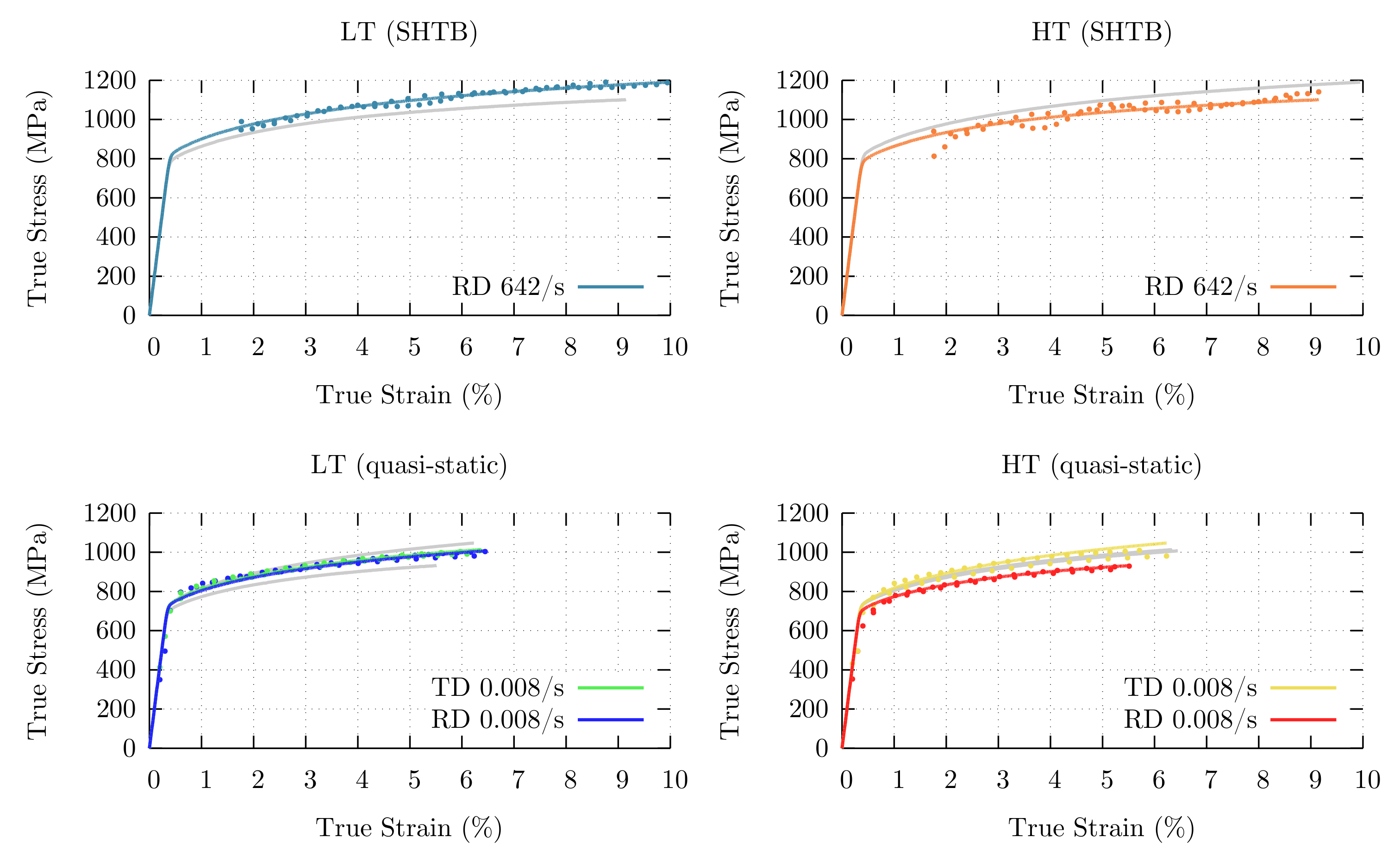
Nine parameters were adjusted using the fitting procedure described in Section 3.6. The quasi-static tensile experiments in rolling and transversal directions, and an additional experiment at high strain rate in the SHTB setup, all of them described in Section 2.3, were used for the fitting. The obtained parameters are listed in Table 4 and simulated tensile curves are compared with the experimental data in Figure 5. Using a single set of fitting parameters for the LT and HT materials, the model is capable of reproducing the experimental results in different directions and strain rates. The difference between the predicted curve and the experimental data points is of the same magnitude as the experimental error in most cases, and even significantly lower for the dynamic experiments, with relatively high experimental scatter. Taking into account the magnitude of the experimental error, a good fitting is obtained. The R 2 value resulting from the combination of all experiments (the six simulations) is of more than 0.94 .

4.3. Formability Properties

Once the model was fitted, it was used as a virtual lab for the realization of several “experiments” with the aim of determining the formability properties of the LT and HT bainitic steels.
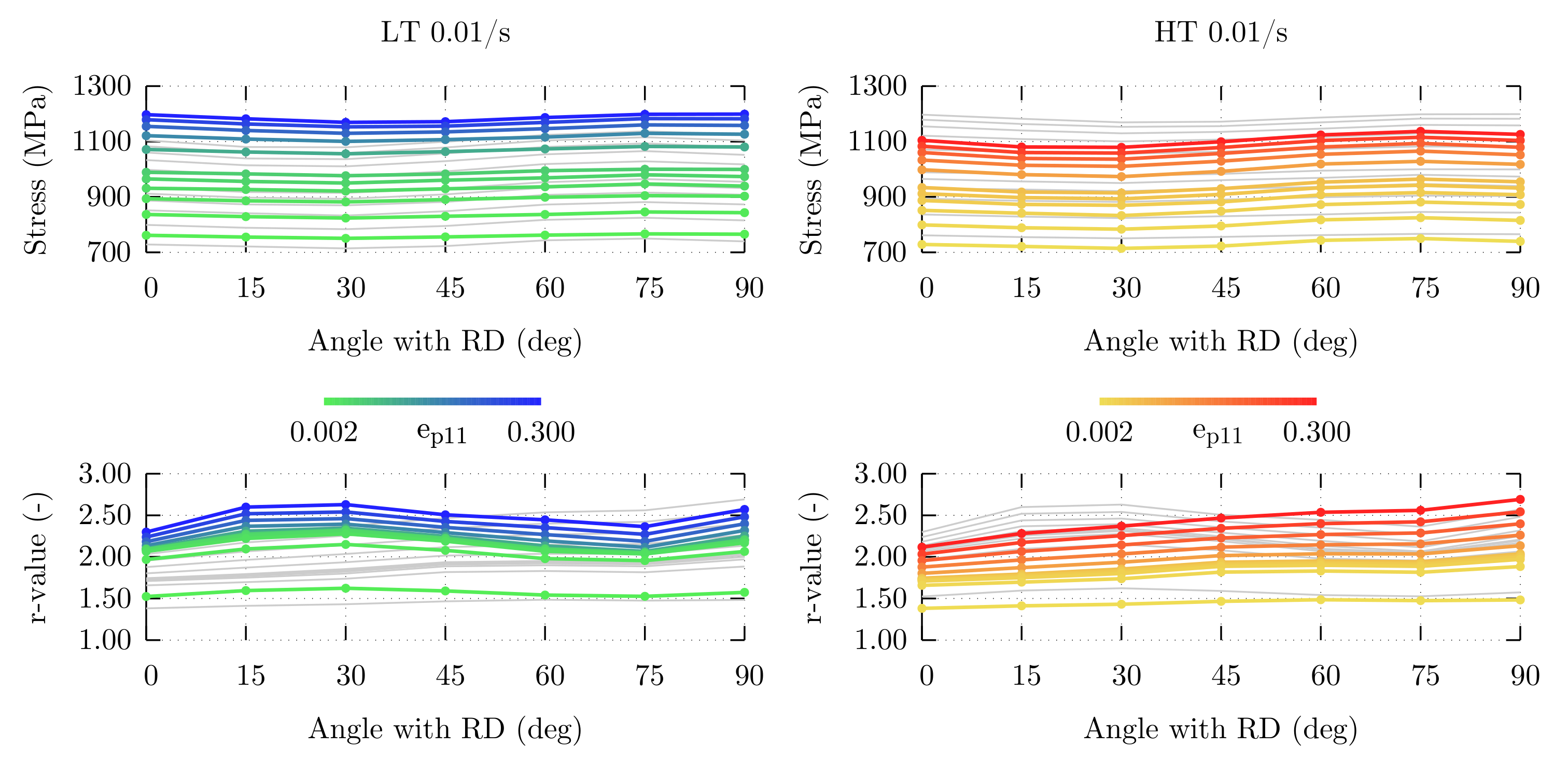
The r-value is calculated, as explained in Section 3.7, using uniaxial tension virtual experiments performed at 15   intervals in directions parallel to the sheet plane, between RD and TD. The calculated r-values for each angle α with respect to RD for different strain levels are shown in Figure 6. The figure also shows the corresponding stress levels. For both materials, these stress levels are very similar for all directions. Only a small decrease around 30   and a similar increase at 75   are observed, slightly more pronounced in the case of the HT material. The trend is the same independently of the applied strain. When looking at the r-values, the anisotropy is more significant for the LT material, where clear peak and valley are distinguished at 15 30   and 75   , respectively. The behavior of the HT material is quite different, with r-values increasing as the loading direction approaches TD. Since there are no large variations in stress and r-value levels depending on loading direction, it can be concluded that the anisotropy of the material is low. Nevertheless, although subtle, the observed differences will have an important impact.
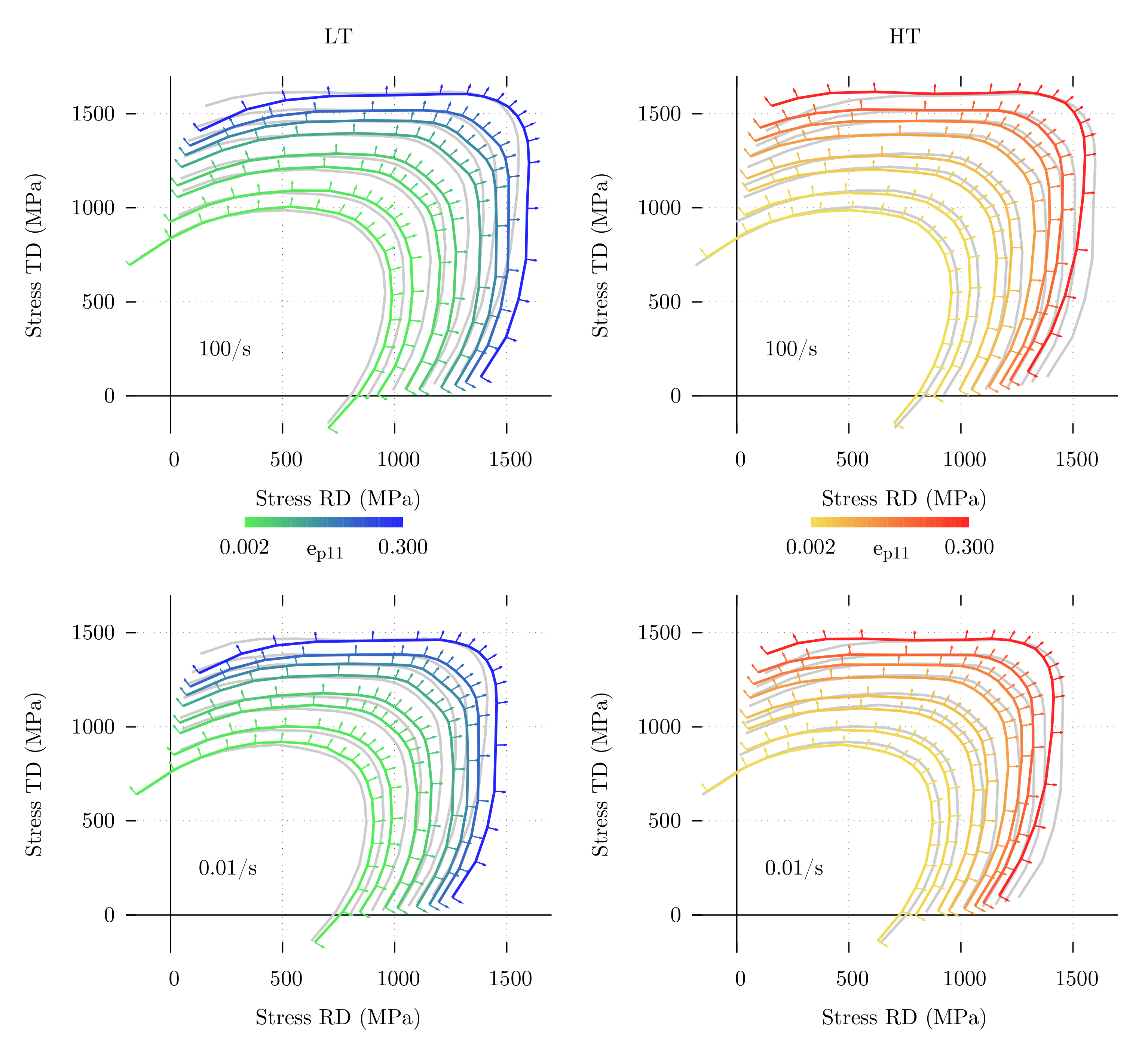
A different set of simulations was performed in which biaxial conditions were imposed, with the goal of calculating yield surfaces and forming limit curves. First, using the uniaxial tests in the RD and TD directions, the θ 0 and θ 90 values were calculated using (23), then simulations were run at regular intervals between both angles. The measured stress levels in directions parallel to RD and TD were then calculated for equal values of plastic work in all the simulations. The isoline obtained for each different value of plastic work corresponds to the projection of the yield surface of the material on the sheet plane for those loading conditions and plastic work value. Obtained yield surfaces corresponding to plastic work levels for specific values of plastic strain during uniaxial tensile deformation along RD, for two different stain rates, are shown in Figure 7. In the figure, both the yield stress and the strain rate direction at that point, indicated by a small vector, can be seen.
At the studied strain rates, both materials initially show a response close to the von Mises criterion at the beginning of plastic deformation. However, as the plastic work increases, the yield surface changes to adopt a shape closer to the one given by Tresca’s criterion. Comparing the yield surfaces of both materials (the results of the other material are represented in each graph using a light grey color), it is seen that this difference is slightly more pronounced for the case of the LT material along TD, while it is more pronounced for the HT material in the direction parallel to RD. Nevertheless, it can be concluded that the response of both materials is very similar. The same trends are observed at quasi-static and high strain rates, but the stress levels are obviously higher at higher strain rates due to the strain rate hardening effect.
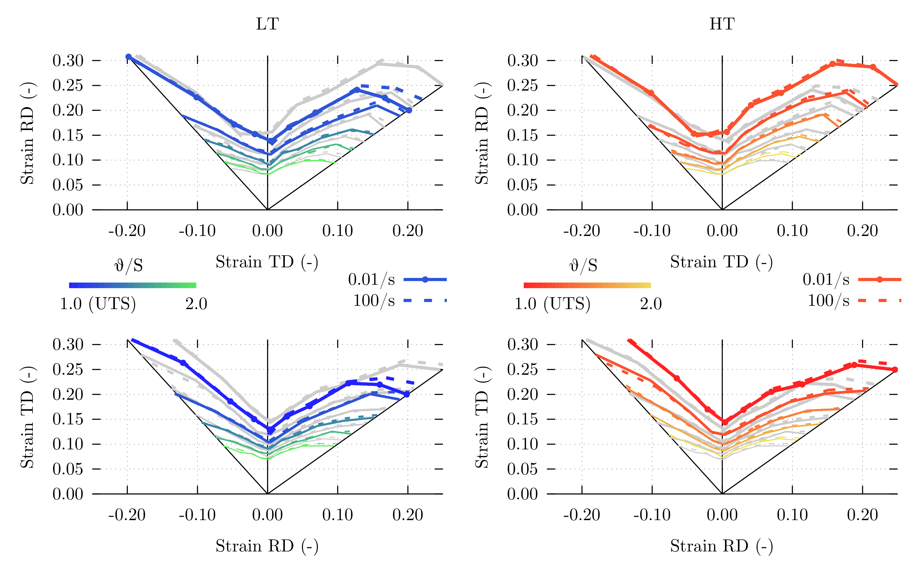
Finally, the results of simulations under biaxial conditions were also used for the calculation of forming limit curves, following the process described in Section 3.7. The forming limit was calculated for principal strains along RD and along TD, for strain rates of 0.01 s 1 and 100 s 1 , giving as a result the diagrams presented in Figure 8. In addition to the forming limit curve at which θ = d S / d e = S (i.e., θ / S = 1 ), curves for several values of θ / S between 1 and 2 are represented in the diagram. This way, the diagram shows not only the forming limit, but also the path followed towards that limit.
The obtained FLCs present the typical shape commonly observed for steel and other sheet metals. The forming limit calculated for the LT material is slightly lower than for the HT one, meaning that it will admit less deformation. It is remarkable that, independently of the material and loading direction, all the curves calculated for θ / S = 2 are very similar. However, as deformation progresses, some differences can be observed. In particular, it is significant that the limit in the vicinity of the biaxial region is much higher when the main loading direction aligns with RD (in the vicinity of the excessive thinning region), but there are no large differences under plane strain conditions. Since the strain hardening effect is affecting both the reached stress and the hardening behavior, a dependence of the FLD on strain rate is not observed.

5. Discussion

It is shown in the previous section that the model presented is capable of reproducing the experimental behavior of the bainitic steels under study with a reduced number of fitting parameters. Moreover, the fitted model was applied to the calculation of formability properties. In this section, the obtained results are analyzed more in depth and compared with results previously reported in the literature.

5.1. Experimental Results and Fitted Parameters

After material characterization, the properties of the steels under study are obtained. The measured grain sizes are not very large, since grain boundaries are defined with a relatively small angle and the bainite and martensite phases present a lath structure. Ellipsoid axes aspect ratios follow a clear distribution around an average value, while the directionality of these ellipsoid appear to be randomly distributed. Regarding crystallographic textures, the results are comparable to typical rolled textures [63,64]. Results of the tensile experiments are shown in Figure 5, together with the fitted curves. The results are in the expected range for the materials studied. While there are bainitic steels with better mechanical properties [65,66], this is usually due to higher carbon content or a nanostructured bainite. Other bainitic steels also with a low carbon content present a similar behavior to the one observed here [67,68].
The fitted parameters are presented in Table 4. Although the fitting algorithm used does not search for the global minimum, using sensible initial values and randomly applying small perturbations to the obtained solutions allows reaching a good fitting. When compared with the experimental scatter, the predicted curves show good accordance with the fitting data.
The first parameter, C 1 , was expected to be of the same order of magnitude of the Taylor factor, and indeed it is very close to a typical Taylor factor value. The value found for the Hall–Petch constant K HP is close to values commonly used for steel (the same constant is being used to account for the Hall–Petch effect of bainite grain size and martensite lath width). The value fitted for α is lower than usual. This may be explained because of the latent hardening coefficients introduced in (18), imprecisions in the measurement of dislocation densities or additional effects not considered in the model. The annihilation distance and β parameter take values that are close to other values in the literature [17]. The carbides shape constant c p and strain rate hardening exponent n take sensible values too. On the other hand, the C 2 and σ imb 2 parameters do not vary too much from the initial values used for the fitting (taken from [17]). These parameters are primarily related with stage IV hardening, and the maximum strain reached in the tensile experiments used for the fitting was relatively low.
It was shown that the presented model with the fitted parameters can reproduce tensile behavior at quasi-static and high strain rates. Since the model relies on a combination of physical principles, general phenomenological relationships and microstructural data, it can be used to simulate a wide range of different materials and loading conditions.

5.2. Role of Microstructural Parameters on Mechanical Behavior

The presented model combines a large number of microstructural parameters in order to predict the behavior of the material. It is possible to use the obtained model to perform simulations to study the effect of different microstructural parameters on mechanical behavior simply changing the value of these parameters.
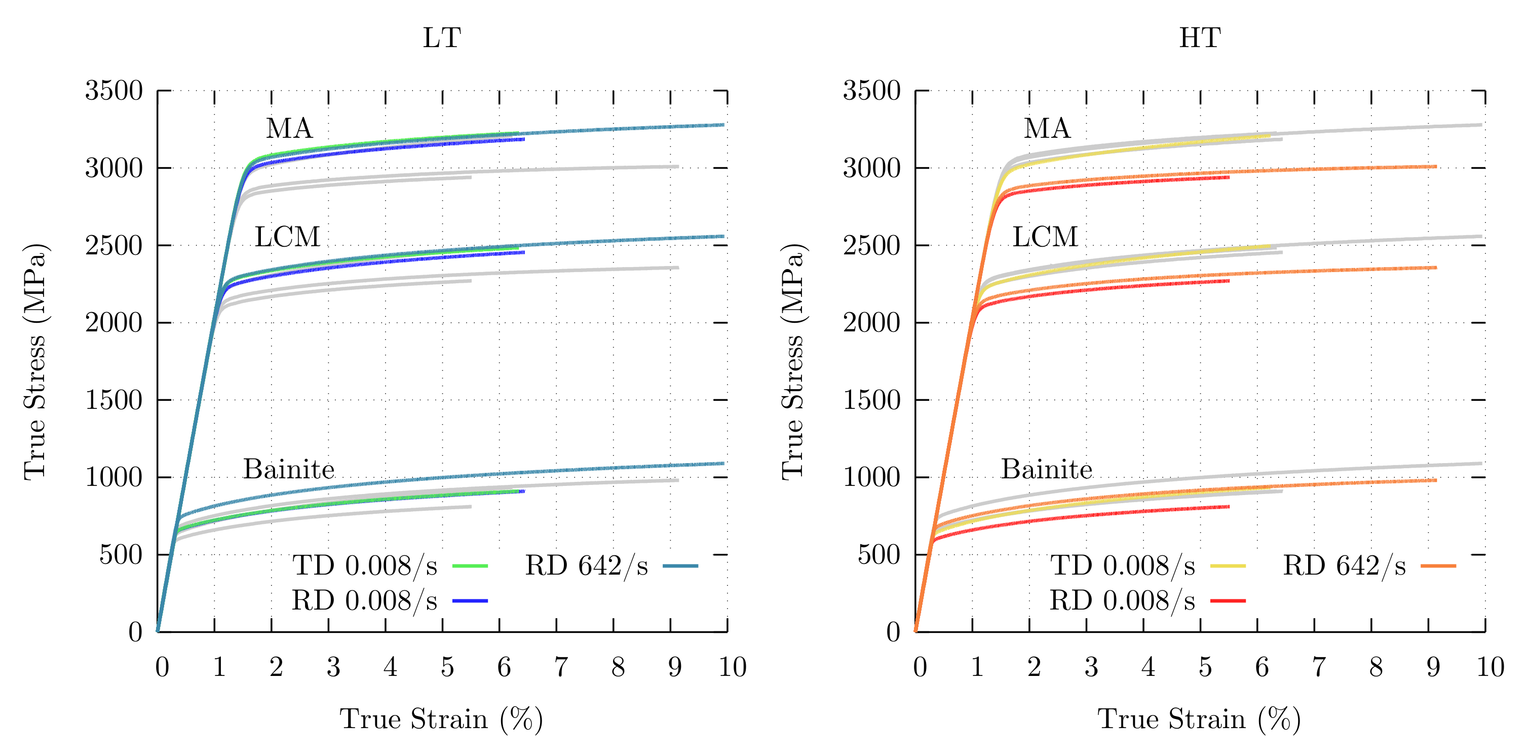
As a first example, Figure 9 shows the independent behavior of the three phases considered in the model. The simulations were performed under the same conditions used for the fitting. Combining experiments along different directions and at different strain rates allows evaluating how strain rate and crystallographic texture affect the response of each of the phases. In the obtained curves, it is clearly observed how the phases with lower yield stress have a larger strain rate sensitivity. While the bainite phase shows a considerable stress increment at higher strain rates, the effect of high strain rate is much lower on the response of the LCM and MA phases. Regarding crystallographic texture, as happened with the experimental and fitted curves, a larger anisotropy is observed for the HT material, especially in the martensitic phases. This result can be correlated with the initial textures in Figure 4. The bainite texture of the LT material exhibits a more homogeneous γ -fiber, while the martensitic phase of the HT material includes some rotated cube components not present in the LT’s ODF which will increase the anisotropy.
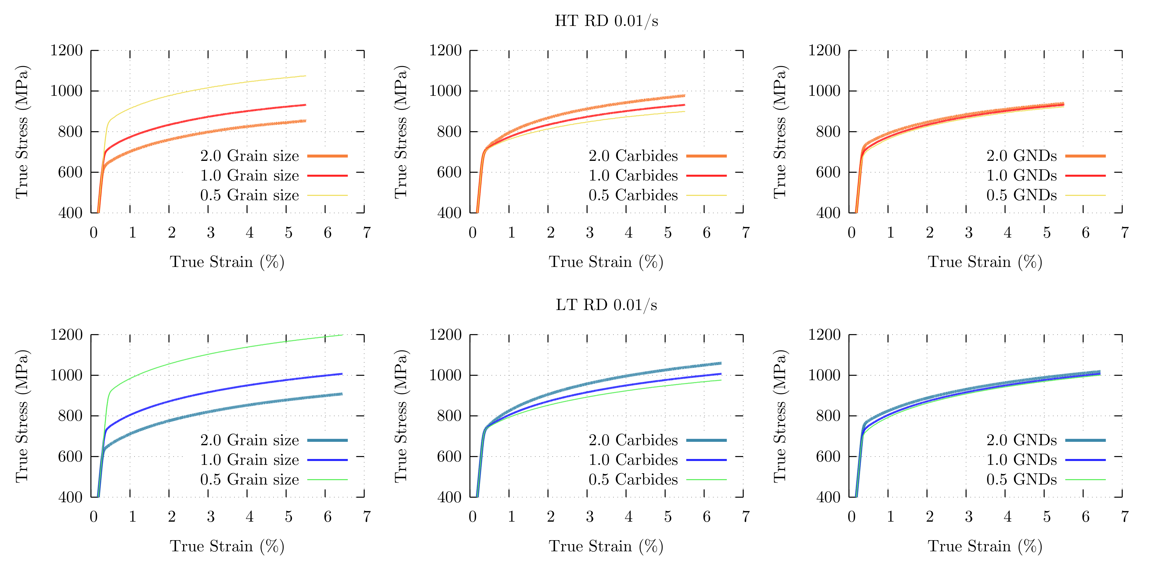
Another example is given in Figure 10. In each graph, three tensile curves are shown, all corresponding to uniaxial tension along RD at a strain rate of 0.008 s 1 . One of the curves is reproduced in Figure 5. The other two curves are calculated modifying the value of a microstructural parameter of the bainitic phase: grain size, initial dislocation density or carbides fraction. In one of the curves, the original value of the parameter (displayed in Table 3) is doubled, and, in the other one, it is halved.
Decreasing the size of the bainite grains makes the material stronger and increasing it makes the material softer, in accordance with the Hall–Petch effect. Grain size also influences the work hardening behavior through Equation (20), but this effect is barely noticed in the graphs. On the other hand, the carbides do not have any effect on the yield stress, but they influence hardening behavior. When the fraction of carbides is higher, the strain hardening effect will be higher too. Since, in Equation (20), the term that accounts for the carbides fraction also includes the carbide shape and carbide size, the effect of doubling the carbides fraction will be the same as the effect of halving the carbides size, and vice versa, while the factor that accounts for the shape of the carbides ( c p ) will have the same effect as the carbides fraction. In the case of dislocation density, there are two different effects on the tensile response. Increasing the dislocation density implies a higher yield stress, but also a slight reduction of the hardening rate. As expected, the effect of doubling or halving the initial dislocation density is small when compared with the effect of doubling the grain size or carbides fraction (N.B. dislocation density values typically vary between several orders of magnitude, while size or fraction values are much closer).
There are many parameters that may be varied too: chemical composition (in particular, carbon content), martensite lath width, grain shape and orientation or crystallographic texture. It is also possible to use the model to optimize these microstructural parameters in order to obtain some desired set of properties, using the same method used for the fitting with an objective set of properties [26,69].

5.3. Formability Properties

As shown in Section 4.3, a large number of simulations under different loading conditions allows performing a detailed characterization of the formability behavior of the material.
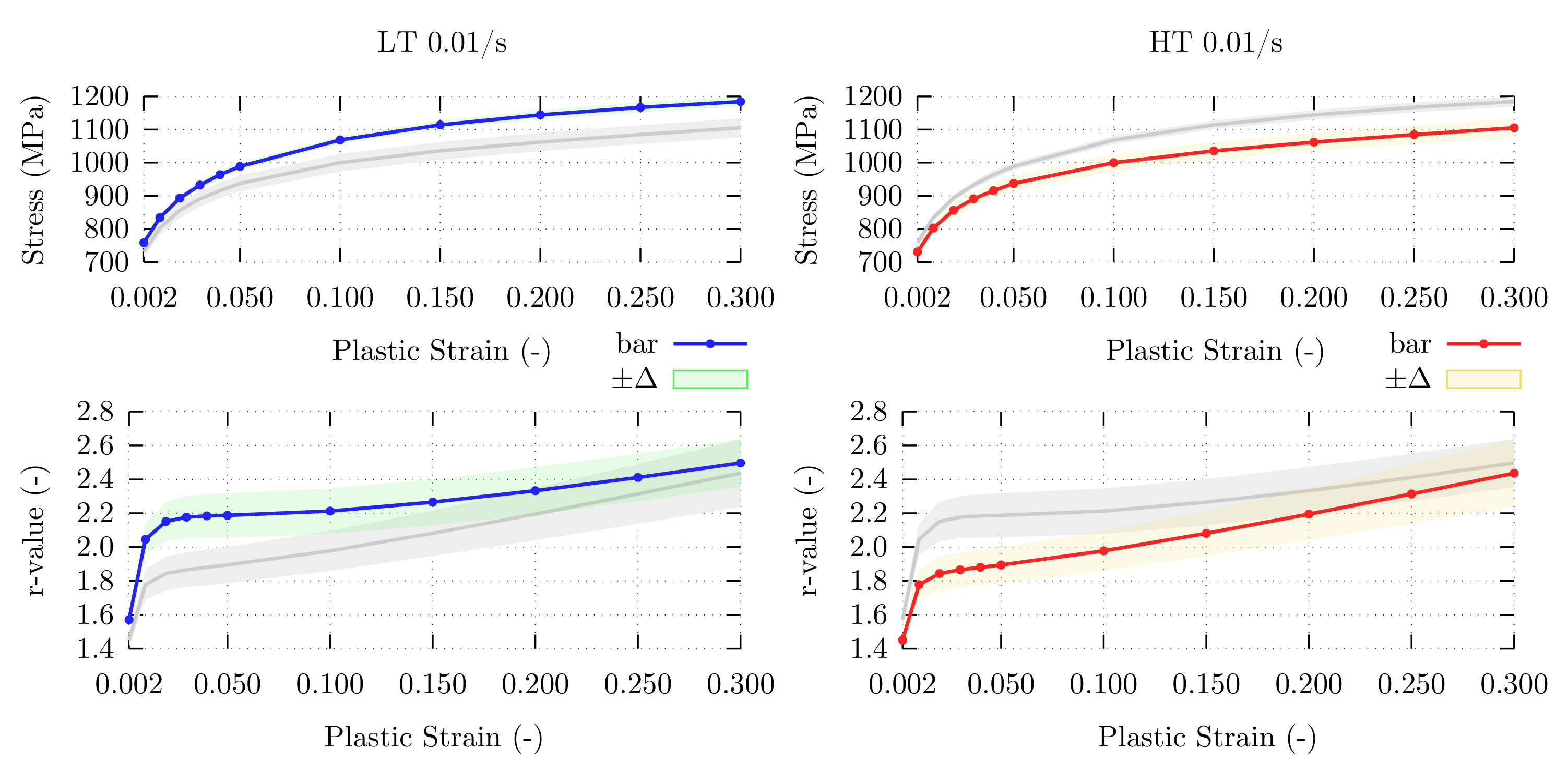
In Figure 6, the r-values or Lankford coefficient and stress levels for different directions and plastic strain values are presented. In order to evaluate the formability of the material, it is convenient to also calculate the aggregate properties r ¯ and Δ r , as explained in Section 3.7. The evolution of r ¯ and Δ r with respect to (uniaxial) plastic strain is presented in Figure 11. The figure also includes curves for the analogous magnitudes σ ¯ and Δ σ , obtained from the stress values in Figure 6.
The graphs show that better formability is obtained for the LT steel. The r ¯ value for LT starts at an upper level and a narrow ± Δ r region is maintained until the end. On the other hand, the HT steel initially has a lower r ¯ value, but it increases as the material hardens. The stress σ ¯ values for the LT steel are also higher than for the HT one. Although the total amount of martensite is almost the same in both materials, and the amount of the MA phase is larger in the HT steel, as Figure 9 shows, the individual phases of LT are stronger. This is the result of smaller grain size, higher carbides content and, depending on loading direction, also of grain shape and crystallographic texture.
Yield surfaces at different strain rates and strain levels are shown in Figure 7. The simulations used to generate these graphs were performed under the same conditions as experimental tests employed for the fitting of phenomenological plasticity models used in finite element simulations [33,34]. In these works, a phenomenological expression of the yield surface is found using biaxial tension experiments on cruciform specimens, and then correlating the measured angles of stress with the strain rate angle. This information can be easily calculated from the simulation results. For instance, Figure 12 shows the curves obtained for the LT and HT steels at a strain rate of 0.01 s 1 .
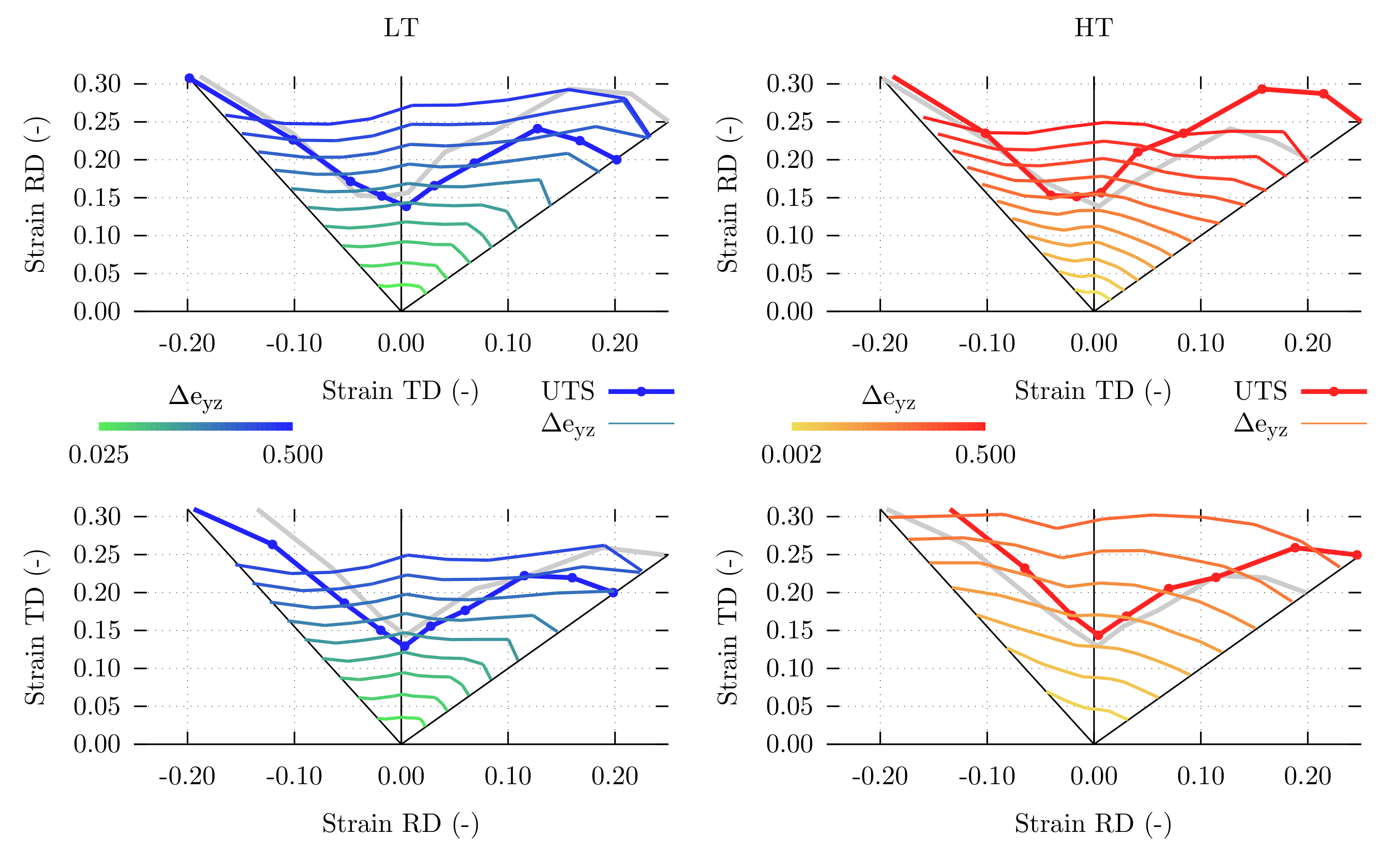
The same experimental data used to calculate yield surfaces can be employed for the calculation of forming limit diagrams, such as the one presented in Figure 8. These forming limits are comparable to previous results in the literature. However, it is important to remark that, most often, finite element simulations with phenomenological models are employed [70,71,72,73]. Instead, the approach used here is based on crystal plasticity, allowing additional analysis that is not possible with a phenomenological model. As an example of possible techniques that could be applied, it is studied how strain inhomogeneities between different grains might be used to investigate the formability of the material. In [74,75], the crystallographic texture around voids in damaged material was identified and clearly differentiated from the texture of grains far from these voids. In [43], a correlation was found between the orientations of grains surrounding the voids and the orientations of the pairs of grains for which a maximum difference was observed in the shear stress component on the plane perpendicular to the loading direction. This maximum difference is calculated by VPSC90 for every simulation step, so it can be easily used to calculate limit curves to be represented in the FLD axis, as shown in Figure 13.
The forming limit curves at 0.01 s 1 of Figure 8 are reproduced again in Figure 13, together with isolevel curves that show the deformation point at which a certain difference is reached between the shear component of two grains in the direction perpendicular to the loading direction. Not only do these curves differ from the forming limit curves calculated from the UTS values, clearly different results are also obtained for the LT and HT steels. The graphs show that, as the loading conditions approach equi-biaxial loading, the forming limit is reached for a larger value of shear difference. Higher differences are also calculated for the LT material. This means that, in accordance with the results of Shakerifard [43], the LT material is more likely to form micro-cracks when deformed than the HT material.

6. Conclusions

An improved version of the VPSC model for the modeling of multiphase advanced high-strength steels is presented. The model extends the VPSC90 elasto-viscoplastic formulation with a new approach to strain rate sensitivity and a work hardening law specifically developed to take into account the microstructural features of advanced high-strength steels. The model can be used for the simulation of the response to mechanical deformation under a wide range of loading conditions for materials with different microstructures.
The obtained model was applied to the study of the formability properties of two different bainitic steels. The capacity to reproduce experimental loading conditions makes it possible to evaluate formability on the basis of methods typically used for experimental characterization, including the calculation of r-values from uniaxial tests in different directions and the calculation of yield surfaces and forming limit diagrams from biaxial tests.

Author Contributions

Conceptualization, J.G.-L. and L.A.I.K.; Investigation, J.G.-L. and B.S.; Methodology, B.S.; Software, J.G.-L.; Supervision, L.A.I.K.; Validation, J.O.-A.; Writing—original draft, J.G.-L.; and Writing—review and editing, B.S., J.O.-A. and L.A.I.K. All authors have read and agreed to the published version of the manuscript.

Funding

This work was carried out in the framework of the BaseForm project. This project has received funding from the European Union’s Research Fund for Coal and Steel (RFCS) research programme under grant agreement #RFCS-CT-2014-00017.

Institutional Review Board Statement

Not applicable.

Informed Consent Statement

Not applicable.

Data Availability Statement

Data is contained within the article.

Acknowledgments

The authors would like to thank all the partners in the BaseForm project, who have provided not only materials and data for this work, but also their experience and their time. The authors would also like to extend this acknowledgment to Ghent University for its collaboration in the realization of SHTB experiments and in the development of the “virtual-lab” tools.

Conflicts of Interest

The authors declare no conflict of interest.

References

  1. Lebensohn, R.A.; Tomé, C. A self-consistent anisotropic approach for the simulation of plastic deformation and texture development of polycrystals: Application to zirconium alloys. Acta Metall. Mater. 1993, 41, 2611–2624. [Google Scholar] [CrossRef]
  2. Segurado, J.; Lebensohn, R.A.; LLorca, J.; Tomé, C.N. Multiscale modeling of plasticity based on embedding the viscoplastic self-consistent formulation in implicit finite elements. Int. J. Plast. 2012, 28, 124–140. [Google Scholar] [CrossRef]
  3. Jeong, Y.; Tomé, C.N. An efficient elasto-visco-plastic self-consistent formulation: Application to steel subjected to loading path changes. Int. J. Plast. 2020, 135, 102812. [Google Scholar] [CrossRef]
  4. Kitayama, K.; Tomé, C.; Rauch, E.; Gracio, J.; Barlat, F. A crystallographic dislocation model for describing hardening of polycrystals during strain path changes. Application to low carbon steels. Int. J. Plast. 2013, 46, 54–69. [Google Scholar] [CrossRef]
  5. Knezevic, M.; McCabe, R.J.; Lebensohn, R.A.; Tomé, C.N.; Liu, C.; Lovato, M.L.; Mihaila, B. Integration of self-consistent polycrystal plasticity with dislocation density based hardening laws within an implicit finite element framework: Application to low-symmetry metals. J. Mech. Phys. Solids 2013, 61, 2034–2046. [Google Scholar] [CrossRef]
  6. Knezevic, M.; McCabe, R.J.; Tomé, C.N.; Lebensohn, R.A.; Chen, S.R.; Cady, C.M.; Gray, G.T., III; Mihaila, B. Modeling mechanical response and texture evolution of α-uranium as a function of strain rate and temperature using polycrystal plasticity. Int. J. Plast. 2013, 43, 70–84. [Google Scholar] [CrossRef]
  7. Zecevic, M.; Knezevic, M. A new visco-plastic self-consistent formulation implicit in dislocation-based hardening within implicit finite elements: Application to high strain rate and impact deformation of tantalum. Comput. Methods Appl. Mech. Eng. 2018, 341, 888–916. [Google Scholar] [CrossRef]
  8. Galán-López, J.; Verleysen, P. Simulation of the plastic response of Ti–6Al–4V thin sheet under different loading conditions using the viscoplastic self-consistent model. Mater. Sci. Eng. A 2018, 712, 1–11. [Google Scholar] [CrossRef]
  9. Lebensohn, R.; Tomé, C.; Castaneda, P.P. Self-consistent modelling of the mechanical behaviour of viscoplastic polycrystals incorporating intragranular field fluctuations. Philos. Mag. 2007, 87, 4287–4322. [Google Scholar] [CrossRef]
  10. Galán, J.; Verleysen, P.; Lebensohn, R. An improved algorithm for the polycrystal viscoplastic self-consistent model and its integration with implicit finite element schemes. Model. Simul. Mater. Sci. Eng. 2014, 22, 055023. [Google Scholar] [CrossRef]
  11. Bhadeshia, H.K. High Performance Bainitic Steels. In Materials Science Forum; Trans Tech Publ: Baech, Switzerland, 2005; Volume 500, pp. 63–74. [Google Scholar]
  12. Garcia-Mateo, C.; Caballero, F.G. Design of carbide-free low-temperature ultra high strength bainitic steels. Int. J. Mater. Res. 2007, 98, 137–143. [Google Scholar] [CrossRef] [Green Version]
  13. Fekete, J. Current challenges in Implementing Advanced High Strength Steels. In Proceedings of the International Conference on Microalloyed Steels: Processing Microstructure, Properties and Peformance, Pittsburgh, PA, USA, 16–19 July 2007; pp. 1–9. [Google Scholar]
  14. Matlock, D.K.; Speer, J.G.; De Moor, E.; Gibbs, P.J. Recent developments in advanced high strength sheet steels for automotive applications: An overview. Jestech 2012, 15, 1–12. [Google Scholar]
  15. Kocks, U. Law for Work-Hardening and Low-Temperature Creep. Trans. ASME J. Eng. Mater. Technol. 1976, 98, 76–85. [Google Scholar] [CrossRef]
  16. Pantleon, W. Stage IV work-hardening related to disorientations in dislocation structures. Mater. Sci. Eng. A 2004, 387, 257–261. [Google Scholar] [CrossRef]
  17. León García, O. Micromechanisms of Failure under Static Loading in Sheet Metals for Automotive Applications. Ph.D. Thesis, Delft University of Technology, Delft, The Netherlands, 2013. [Google Scholar]
  18. Zhu, K.; Bouaziz, O.; Oberbillig, C.; Huang, M. An approach to define the effective lath size controlling yield strength of bainite. Mater. Sci. Eng. A 2010, 527, 6614–6619. [Google Scholar] [CrossRef]
  19. Ashby, M. The deformation of plastically non-homogeneous materials. Philos. Mag. A J. Theor. Exp. Appl. Phys. 1970, 21, 399–424. [Google Scholar] [CrossRef]
  20. Zuev, L.B. On the waves of plastic flow localization in pure metals and alloys. Ann. Phys. 2007, 16, 286–310. [Google Scholar] [CrossRef]
  21. Shakerifard, B.; Lopez, J.G.; Legaza, M.C.T.; Verleysen, P.; Kestens, L.A. Strain rate dependent dynamic mechanical response of bainitic multiphase steels. Mater. Sci. Eng. A 2019, 745, 279–290. [Google Scholar] [CrossRef]
  22. Asaro, R.J.; Needleman, A. Overview no. 42 texture development and strain hardening in rate dependent polycrystals. Acta Metall. 1985, 33, 923–953. [Google Scholar] [CrossRef]
  23. Johnson, G.; Cook, W. A Constitutive modeling and data for metals subjected to large strain rates and high temperatures. In Proceedings of the 7th International Symposium on Ballistics, Hague, The Netherlands, 19–21 April 1983; pp. 541–577. [Google Scholar]
  24. Banabic, D.; Barlat, F.; Cazacu, O.; Kuwabara, T. Advances in anisotropy of plastic behaviour and formability of sheet metals. Int. J. Mater. Form. 2020, 13, 749–787. [Google Scholar] [CrossRef]
  25. Lankford, W. New criteria for predicting the performance of deep drawing sheets. Trans. ASM 1950, 42, 1197. [Google Scholar]
  26. Galán-López, J.; Kestens, L.A. Optimization of crystallographic texture for sheet-forming applications using Taylor-based Models. Metall. Mater. Trans. A 2018, 49, 5745–5762. [Google Scholar] [CrossRef] [Green Version]
  27. Van Houtte, P.; Li, S.; Engler, O. Taylor-Type Homogenization Methods for Texture and Anisotropy. In Continuum Scale Simulation of Engineering Materials: Fundamentals–Microstructures–Process Applications; Wiley: Weinheim, Germany, 2004; pp. 459–472. [Google Scholar]
  28. Ma, A.; Roters, F.; Raabe, D. Simulation of Textures and Lankford Values for Face Centered Cubic Polycrystaline Metals by Using a Modified Taylor Model; Max-Planck-Institut für Eisenforschung: Düsseldorf, Alemanha, 2004. [Google Scholar]
  29. Melchior, M.A.; Remacle, J.F.; Delannay, L. Assessment of adaptative meshing in CPFEM simulation of the anisotropy of polycristalline aggregates. In Proceedings of the 8th World Congress on Computational Mechanics, Venice, Italy, 30 June–5 July 2008. [Google Scholar]
  30. Hammami, W.; Delannay, L.; Habraken, A.M.; Duchêne, L. Crystal plasticity prediction of Lankford coefficients using the MULTISITE model: Influence of the critical resolved shear stresses. Int. J. Mater. Form. 2009, 2, 65–68. [Google Scholar] [CrossRef]
  31. Min, K.; Jeong, W.; Hong, S.; Lee, C.; Cha, P.R.; Han, H.; Lee, M.G. Integrated crystal plasticity and phase field model for prediction of recrystallization texture and anisotropic mechanical properties of cold-rolled ultra-low carbon steels. Int. J. Plast. 2020, 127, 102644. [Google Scholar] [CrossRef]
  32. Cazacu, O.; Barlat, F. A criterion for description of anisotropy and yield differential effects in pressure-insensitive metals. Int. J. Plast. 2004, 20, 2027–2045. [Google Scholar] [CrossRef]
  33. Kuwabara, T.; Ikeda, S.; Kuroda, K. Measurement and analysis of differential work hardening in cold-rolled steel sheet under biaxial tension. J. Mater. Process. Technol. 1998, 80, 517–523. [Google Scholar] [CrossRef]
  34. Coppieters, S.; Hakoyama, T.; Debruyne, D.; Takahashi, S.; Kuwabara, T. Inverse Yield Locus Identification of Sheet Metal Using a Complex Cruciform in Biaxial Tension and Digital Image Correlation. Proceedings 2018, 2, 382. [Google Scholar] [CrossRef] [Green Version]
  35. Plunkett, B.; Lebensohn, R.; Cazacu, O.; Barlat, F. Anisotropic yield function of hexagonal materials taking into account texture development and anisotropic hardening. Acta Mater. 2006, 54, 4159–4169. [Google Scholar] [CrossRef]
  36. Inal, K.; Mishra, R.K.; Cazacu, O. Forming simulation of aluminum sheets using an anisotropic yield function coupled with crystal plasticity theory. Int. J. Solids Struct. 2010, 47, 2223–2233. [Google Scholar] [CrossRef] [Green Version]
  37. Gawad, J.; Banabic, D.; Van Bael, A.; Comsa, D.S.; Gologanu, M.; Eyckens, P.; Van Houtte, P.; Roose, D. An evolving plane stress yield criterion based on crystal plasticity virtual experiments. Int. J. Plast. 2015, 75, 141–169. [Google Scholar] [CrossRef]
  38. Marciniak, Z.; Kuczyński, K. Limit strains in the processes of stretch-forming sheet metal. Int. J. Mech. Sci. 1967, 9, 609–620. [Google Scholar] [CrossRef]
  39. Jacques, N. An analytical model for necking strains in stretched plates under dynamic biaxial loading. Int. J. Solids Struct. 2020, 200, 198–212. [Google Scholar] [CrossRef]
  40. Savoie, J.; Jain, M.; Carr, A.; Wu, P.; Neale, K.; Zhou, Y.; Jonas, J. Predictions of forming limit diagrams using crystal plasticity models. Mater. Sci. Eng. A 1998, 257, 128–133. [Google Scholar] [CrossRef]
  41. Hajian, M.; Assempour, A. Experimental and numerical determination of forming limit diagram for 1010 steel sheet: A crystal plasticity approach. Int. J. Adv. Manuf. Technol. 2015, 76, 1757–1767. [Google Scholar] [CrossRef]
  42. Wu, P.; Neale, K.; Van der Giessen, E.; Jain, M.; MacEwen, S.; Makinde, A. Crystal plasticity forming limit diagram analysis of rolled aluminum sheets. Metall. Mater. Trans. A 1998, 29, 527–535. [Google Scholar] [CrossRef] [Green Version]
  43. Shakerifard, B. From Micro-Mechanisms of Damage Initiation to Constitutive Mechanical Behavior of Bainitic Multiphase Steels. Ph.D. Thesis, Delft University of Technology, Delft, The Netherlands, 2019. [Google Scholar]
  44. Ruhl, R.; Cohen, M. Splat quenching of iron–carbon alloys. Trans. Metall. Soc. AIME 1969, 245, 241–251. [Google Scholar]
  45. Van Houtte, P. A new method for the determination of texture functions from incomplete pole figures—Comparison with older methods. Textures Microstruct. 1984, 6, 137–161. [Google Scholar] [CrossRef] [Green Version]
  46. Verleysen, P.; Degrieck, J.; Verstraete, T.; Van Slycken, J. Influence of specimen geometry on split Hopkinson tensile bar tests on sheet materials. Exp. Mech. 2008, 48, 587. [Google Scholar] [CrossRef]
  47. Kolsky, H. An investigation of the mechanical properties of materials at very high rates of loading. Proc. Phys. Soc. Sect. B 1949, 62, 676. [Google Scholar] [CrossRef]
  48. Peirs, J. Experimental Characterisation and Modelling of the Dynamic Behaviour of the Titanium Alloy Ti6Al4V (’Experimentele Karakterisering en Modellering van het Dynamisch Materiaalgedrag van de Titaniumlegering Ti6Al4V’). Ph.D. Thesis, Ghent University, Ghent, Belgium, 2012. [Google Scholar]
  49. Tomé, C.; Lebensohn, R. Manual for Code Visco-Plastic Self-Consistent (vpsc); Los Alamos National Laboratory: Los Alamos, NM, USA, 2009. [Google Scholar]
  50. Schmid, E.; Boas, W. Kristallplastizität: Mit Besonderer Berücksichtigung der Metalle; Springer: Berlin/Heidelberg, Germany, 2013; Volume 17. [Google Scholar]
  51. Ramazani, A.; Pinard, P.; Richter, S.; Schwedt, A.; Prahl, U. Characterisation of microstructure and modelling of flow behaviour of bainite-aided dual-phase steel. Comput. Mater. Sci. 2013, 80, 134–141. [Google Scholar] [CrossRef]
  52. He, S.; He, B.; Zhu, K.; Huang, M. Evolution of dislocation density in bainitic steel: Modeling and experiments. Acta Mater. 2018, 149, 46–56. [Google Scholar] [CrossRef]
  53. Gutierrez, I. Mechanical Property Models for High-Strength Complex Microstructures; Office for Official Publications of the European Communities: Luxembourg, 2008. [Google Scholar]
  54. Pickering, F.B. Physical Metallurgy and the Design of Steels; Applied Science Publishers Ltd.: London, UK, 1978. [Google Scholar]
  55. Gutiérrez, I.; Altuna, M.A. Work-hardening of ferrite and microstructure-based modelling of its mechanical behaviour under tension. Acta Mater. 2008, 56, 4682–4690. [Google Scholar] [CrossRef]
  56. Hall, E. The deformation and ageing of mild steel: III discussion of results. Proc. Phys. Soc. Sect. B 1951, 64, 747. [Google Scholar] [CrossRef]
  57. Petch, N. The cleavage strength of polycrystals. J. Iron Steel Inst. 1953, 174, 25–28. [Google Scholar]
  58. Kim, S.A.; Johnson, W.L. Elastic constants and internal friction of martensitic steel, ferritic-pearlitic steel, and α-iron. Mater. Sci. Eng. A 2007, 452, 633–639. [Google Scholar] [CrossRef]
  59. Franciosi, P. Glide mechanisms in bcc crystals: An investigation of the case of α-iron through multislip and latent hardening tests. Acta Metall. 1983, 31, 1331–1342. [Google Scholar] [CrossRef]
  60. Pathak, N.; Butcher, C.; Worswick, M.J.; Bellhouse, E.; Gao, J. Damage evolution in complex-phase and dual-phase steels during edge stretching. Materials 2017, 10, 346. [Google Scholar] [CrossRef] [Green Version]
  61. Smith, D.A. Die Design Handbook; Society of Manufacturing Engineers: Southfield, MI, USA, 1990. [Google Scholar]
  62. Van Houtte, P. MTM-FHM Software, Ver. 2.; User Manual; Peatix: Tokyo, Japan, 1995. [Google Scholar]
  63. Kestens, L.; Pirgazi, H. Texture formation in metal alloys with cubic crystal structures. Mater. Sci. Technol. 2016, 32, 1303–1315. [Google Scholar] [CrossRef] [Green Version]
  64. Hernandez-Duran, E.; Ros-Yanez, T.; Castro-Cerda, F.; Petrov, R. The influence of the heating rate on the microstructure and mechanical properties of a peak annealed quenched and partitioned steel. Mater. Sci. Eng. A 2020, 797, 140061. [Google Scholar] [CrossRef]
  65. Kumar, A.; Singh, A. Mechanical properties of nanostructured bainitic steels. Materialia 2021, 15, 101034. [Google Scholar] [CrossRef]
  66. Li, Q.; Zhang, Y.; Li, W.; Huang, X.; Huang, W. Improved mechanical properties of a quenched and partitioned medium-carbon bainitic steel by control of bainitic isothermal transformation. J. Mater. Eng. Perform. 2020, 29, 32–41. [Google Scholar] [CrossRef]
  67. Ivaniski, T.M.; Souza, T.F.D.; Épp, J.; Rocha, A.d.S. Constitutive Modelling of High Temperature Flow Behaviour for a Low Carbon High Silicon Bainitic Steel. Mater. Res. 2020, 23. [Google Scholar] [CrossRef]
  68. Mousalou, H.; Yazdani, S.; Avishan, B.; Ahmadi, N.P.; Chabok, A.; Pei, Y. Microstructural and mechanical properties of low-carbon ultra-fine bainitic steel produced by multi-step austempering process. Mater. Sci. Eng. A 2018, 734, 329–337. [Google Scholar] [CrossRef]
  69. Fullwood, D.T.; Niezgoda, S.R.; Adams, B.L.; Kalidindi, S.R. Microstructure sensitive design for performance optimization. Prog. Mater. Sci. 2010, 55, 477–562. [Google Scholar] [CrossRef]
  70. Bhargava, M.; Tewari, A.; Mishra, S.K. Forming limit diagram of Advanced High Strength Steels (AHSS) based on strain-path diagram. Mater. Des. 2015, 85, 149–155. [Google Scholar] [CrossRef]
  71. Basak, S.; Panda, S.K. Implementation of YLD-96 plasticity theory in formability analysis of Bi-axial pre-strained steel sheets. Procedia Eng. 2017, 173, 1085–1092. [Google Scholar] [CrossRef]
  72. Bandyopadhyay, K.; Basak, S.; Prasad, K.S.; Lee, M.G.; Panda, S.K.; Lee, J. Improved formability prediction by modeling evolution of anisotropy of steel sheets. Int. J. Solids Struct. 2019, 156, 263–280. [Google Scholar] [CrossRef]
  73. Achineethongkham, K.; Uthaisangsuk, V. Analysis of forming limit behaviour of high strength steels under non-linear strain paths using a micromechanics damage modelling. Int. J. Mech. Sci. 2020, 183, 105828. [Google Scholar] [CrossRef]
  74. Shakerifard, B.; Galan Lopez, J.; Kestens, L.A. A New Electron Backscatter Diffraction-Based Method to Study the Role of Crystallographic Orientation in Ductile Damage Initiation. Metals 2020, 10, 113. [Google Scholar] [CrossRef] [Green Version]
  75. Shakerifard, B.; Lopez, J.G.; Hisker, F.; Kestens, L. Crystallographically resolved damage initiation in advanced high strength steel. In Proceedings of the IOP Conference Series: Materials Science and Engineering, Kuala Lumpur, Malaysia, 13–14 August 2018; IOP Publishing: Bristol, UK, 2018; Volume 375, p. 012022. [Google Scholar]
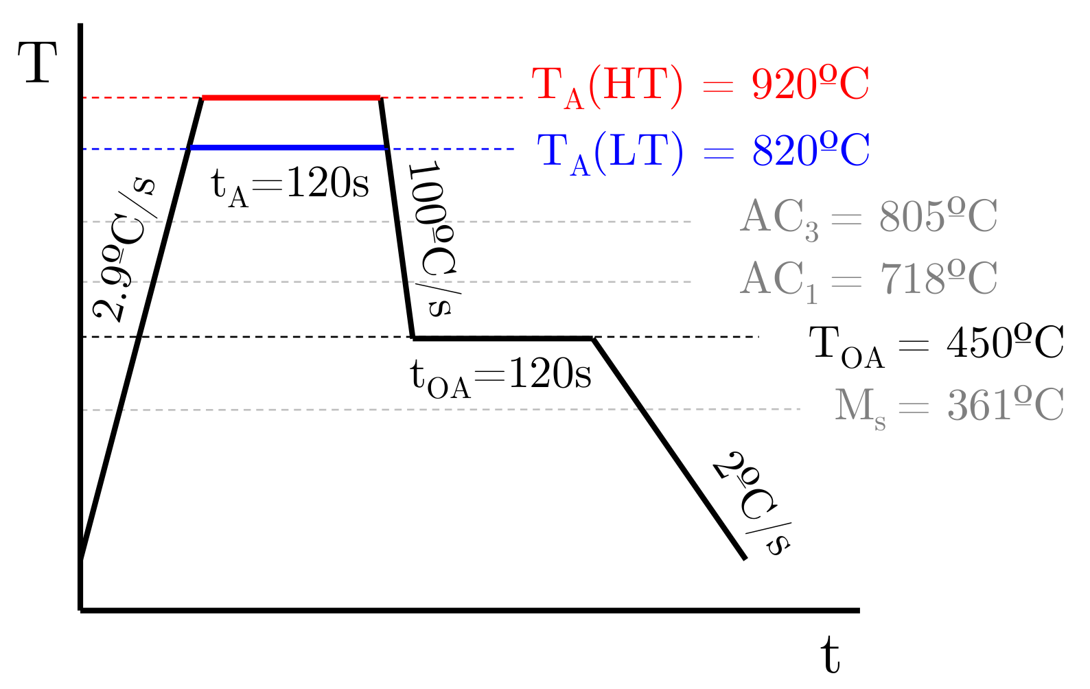
Figure 1. Heat treatments applied to obtain the LT and HT bainitic steels. The material was first heated up to the austenization temperature ( 100   C more for HT), cooled down at a fast rate, and held for 2 min at the overaging temperature before final cooling at a slower rate.
Applsci 11 06122 g001
Figure 2. SEM micrographs of the two bainitic steels obtained after the heat treatments in Figure 1: (a) HT; and (b) LT. The images show the presence MA islands (larger bright areas) and carbides in the bainitic matrix (small bright particles).
Applsci 11 06122 g002
Figure 3. Distribution of grain sizes (equivalent diameter), aspect ratio (of the equivalent ellipsoid axes) and orientation (of the equivalent ellipsoid, not crystallographic) calculated from EBSD experiments for the LT and HT steels.
Applsci 11 06122 g003
Figure 4. Crystallographic textures of the bainite and martensite phases calculated from EBSD experiments for the LT and HT steels. The φ 2 = 45   section of the ODF is shown for the bainitic and martensitic phases of each steel. The ODFs were calculated using MTM-FHM software [62] (with L max = 22 and a Gaussian spread of 7   ). Intensity levels are displayed over the contour lines.
Applsci 11 06122 g004
Figure 5. Fitting of experimental tensile curves corresponding to quasi-static experiments in the rolling and transversal directions (bottom row) and at high strain rate in the rolling direction (top row). The combined R 2 value is 0.944 . The fitted parameters are listed in Table 4.
Applsci 11 06122 g005
Figure 6. Uniaxial stress and r-values along different directions on the sheet plane for different values of uniaxial plastic strain for the LT and HT steels.
Applsci 11 06122 g006
Figure 7. Yield surface and strain rate direction at different plastic work levels and strain rates of 0.01 and 100 s 1 for the LT and HT steels. The legend indicates uniaxial plastic strain during tensile deformation along the RD direction for that level of plastic work.
Applsci 11 06122 g007
Figure 8. Forming limit diagrams at strain rates of 0.01 and 100 s 1 for the LT and HT steels, calculated for different values of θ / S (with θ = d S / d e ). The curve calculated for the UTS point ( θ / S = 1 ) is shown with points too.
Applsci 11 06122 g008
Figure 9. Tensile diagrams of individual phases in the LT and HT materials under the same loading conditions used in the fitting (cf. Figure 5).
Applsci 11 06122 g009
Figure 10. Influence of bainite microstructural parameters ((left) grain size; (middle) carbides fraction; and (right) initial dislocation density) on the tensile behavior of the LT and HT materials at a strain rate of 0.01 s 1 along RD.
Applsci 11 06122 g010
Figure 11. Predicted evolution of r ¯ ± Δ r and σ ¯ ± Δ σ with respect to uniaxial plastic strain for the LT and HT steels calculated from the values in Figure 6.
Applsci 11 06122 g011
Figure 12. Angle of strain rate with respect to loading direction for the LT and HT steels at a strain rate of 0.01 s 1 , calculated from the yield surfaces in Figure 7.
Applsci 11 06122 g012
Figure 13. Forming limit diagrams superimposed with isolevel lines indicating the maximum difference on the shear strain component perpendicular to the loading direction between two grains.
Applsci 11 06122 g013
Table 1. Chemical composition of the steel under study.
ElementCMnSiCrAlPSNFe
Weight (%)0.2151.960.100.610.0200.0070.00270.005Remaining
Table 2. Latent hardening coefficients for BCC metals taken from Franciosi [59].
a ss { 110 } 111 { 112 } 111
{ 110 } 111 3.05.2
{ 112 } 111 5.25.1
Table 3. Microstructural parameters for bainite, low carbon martensite and martensite–austenite islands: v f is the volume fraction of the phase, d is the size (grain diameter for bainite and lath width for martensite), A.R. is the aspect ratio, ρ is the dislocation density, W C is the carbon content (in weight percent) and v c and d c are, respectively, the volume fraction and size of carbides.
MaterialPhase v f (%)d ( μ m)A.R. (-) ρ ( m 2 ) W C (%) v c (%) d c ( μ m)
HTBainite 91.8 1.44 0.42 1.45 · 10 14 0.03 3.8 0.07
Martensite (LCM) 4.8 0.50 0.44 1.72 · 10 14 0.28 1.8 0.07
Martensite (MA) 3.4 0.70 0.44 1.72 · 10 14 0.44 0
LTBainite 91.4 1.17 0.42 1.56 · 10 14 0.03 3.3 0.07
Martensite (LCM) 6.2 0.47 0.44 1.88 · 10 14 0.28 1.5 0.07
Martensite (MA) 2.4 0.60 0.44 1.88 · 10 14 0.44 0
Table 4. Fitted parameters: Proportionality constant C 1 , Hall–Petch constant K H , dislocations annihilation distance y, dislocations structure constants α and β , constants related with stage IV hardening C 2 and σ imb 2 , carbides shape constant c p and strain rate sensitivity exponent in the viscoplastic equation n. The combined R 2 value is 0.944 . The fitted curves are shown in Figure 5.
C 1 ( ) K HP ( ) α ( ) β ( ) y ( nm ) C 2 ( μ m 2 ) σ imb 2 ( μ m 2 ) c p ( ) n ( )
2.42 9.12 0.05 5.07 6.35 0.017 0.500 8.78 17.78
Publisher’s Note: MDPI stays neutral with regard to jurisdictional claims in published maps and institutional affiliations.