Effect of the Rolling Friction on the Heap Formation of Dry and Wet Coarse Discs

Abstract

We performed 2D numerical simulations to study the dynamic heap formation of coarse particles in different dry and wet conditions. Our results show that the dynamics of the particles depend not only on the amount of liquid contained in the bulk, but also on the initial particles packing, i.e., the arrangement of the grains. The wet particles cohesion model effect on coarse discs heap formation is minimal. This effect is mostly noticed in the particle arrangement and the energy variation rather than the heap formation. We found that the energy of the system varies with the liquid content up to a threshold value, equal to 219% in our study, where the influences of the parameters are minimal. At high liquid volume, the final pile height and radius tend towards an asymptotic value. The initial particles arrangement has a significant impact on the behavior of the bulk after the opening of the lateral walls. The number of particles in the triangle, formed by the initial width of the packing as a base and with a depth equal to N × D, with N representing the number of particles on a vertical line and D their diameter, influences the final shape of the pile. Indeed, the larger the number, the smaller the height of the pile. The simulations performed with the same initial packing show that the cohesion and capillary forces reduce the bulk kinetic energy and increase the potential energy when used with the elastic-plastic spring dashpot model. For the directional constant model, the dependance of the torque on the normal force and the particle size explains that there is almost no difference between the dry and wet model regarding energies. Finally, the elastic-plastic spring-dashpot model is more efficient in reducing the kinetic energy of the system and producing stable piles. Our simulation results using glass beads are in good agreement with the experiments.

1. Introduction

Granular materials are among the most used materials in engineering projects. They are bulk materials composed of powders with particle sizes varying from 0.1 to 100 µm and granular solids with diameters ranging from 100 to 3000 µm [1], and after the fluids, they are the second most used material in the industry [2]. Thus, we often have to use numerical methods to study numerous engineering problems related to them: flow through hoppers, slope stability, geotechnical tests, and so on. Models using continuum assumptions were first used to study granular materials. Still, they cannot represent local discontinuities, which play a fundamental role in their behavior [3]. Nowadays, the DEM is widely used in soil mechanics. First introduced by Cundall [4] in 1979, DEM considers the material as an assembly of particles free to interact with other particles. It allows us to have a set of data at each time step, including particle positions, interaction forces, torques, etc. This particular approach is essential to the understanding of the relation between the microscopic and macroscopic parameters. A lot of researchers have shown its efficiency to study granular materials and particle flow [5,6], even though the application of DEM to natural materials still requires further development [7].

The angle of repose is an important macroscopic parameter in characterizing granular materials’ behavior, mainly for slope stability issues and the design of retaining structures [8]. Although its definition is not always straightforward and depends on the application and the material’s behavior, we distinguish two types of repose angle: static and dynamic [9]. Different methods have been used to determine the angle of repose of materials, but there is no standardization [10]. Among them, we can cite the tilting box method, fixed funnel method, revolving cylinder/drum method, hollow cylinder method, and tilting cylinder method [9,11].

Column collapse is a good way to study granular materials under different regimes as well as the formation of the final heap. Because of its simplicity, both numerically and experimentally, it has become a preferential way for researchers to study particles. Despite its apparent simplicity, it makes the grains go through all kinetic phases: static before the opening of the sidewalls followed by the triggering phase, dynamic flow after the opening of the walls, and ends up with the jamming state.

In DEM, we usually use heap formation experiments to calibrate the numerical simulation models [12,13,14]. This method allows researchers to ensure the accuracy of the input parameters and the simulation results. The particle properties are not easy to determine experimentally. Two types of calibration are used. In direct calibration, the simulation is calibrated by empirically measuring the particle properties and then using them as the simulation inputs. In reverse calibration, a bulk property is measured, such as the distribution of particle size, bulk (packing) density, and repose angle. Then, a set of simulation parameters is changed until the measured bulk properties are matched [15]. However, the microscopical and macroscopical behavior of the particles during heap formation simulations involving a dynamic phase are not totally understood.

One of the most promising areas of DEM is the numerical study of wet granular materials. Some researches have been carried out in this field and show that it is a reliable tool to investigate wet particle media. Nguyen et al. [16] studied the attraction between particles of different diameters and the damage ratio using a cohesion contact model, including the Van Der Waals forces. Yuki and Daiki [17] developed a contact force model which includes the liquid bridge force for wet particle simulation. Despite many assumptions, their study of glass beads’ behavior in pan pelletizer shows fair agreements between their simulation and experiment, proving that their model can be used to simulate cohesion forces between particles. DEM has also been used to study the collapse of wet granular column [18], erosion process in partially wet sand [19], and angle of repose of wet sand [20]. Staron and Hinch [21] investigated the dynamics of granular material column collapse and the effect of initial particle arrangement using the contact dynamics method. They discovered that the aspect ratio has a major impact on the final form of the pile in dry conditions.

In this paper, we study the heap formation of dry and wet coarse soil. Three models of rolling friction torque are introduced and used to examine the stability of the heap. We propose a simulation method that can simulate the formation of a stable pile of monosized discs under two-dimensional conditions and allow a good insight into the heap formation process. Throughout this study, rolling friction torque based on the experimental and theoretical analysis of [22,23] was used. Finally, we investigated the influence of the rolling friction model on the stability and the energy variation during all the phases. The proposed model’s validity is ensured by a good agreement between the simulation results and experiments we performed using glass beads.

2. Materials and Methods

2.1. Contact Force Model

This study is based on DEM proposed by Cundall and Stark [4]. The Newton second law defines each particle’s movement, and particle motion is the result of its interaction with neighboring particles or walls and the action of other external forces. With an appropriate time step, all forces and torques can be determined from the interactions between the particle and its immediate neighbors [23]. We selected a time step equal to 0.01 of the critical time step which depends on the normal stiffness, the damping coefficient, and the particle mass [6].

$$\Delta t_c=\frac{\pi }{\sqrt{\frac{S_n}{m}\left(1-z_n^2\right)}}$$

where $\Delta t_c$ is the critical time step, $S_n$ the normal stiffness, $m$ the particle mass, and $z_n$ the dimensionless damping coefficient.

Particles are allowed to have small overlaps while in contact. The translational and rotational movements of particle $i$ which is in contact with $k$ particles at time $t$ can be described by the following equations:

$$m_i\frac{d{\mathit{V}}_{\mathit{i}}}{dt}=m_i\mathit{g}+{\displaystyle \sum }_{j=1}^k{\mathit{F}}_{\mathit{i}\mathit{j}}$$

(1)

$$I_i\frac{d{\mathit{\omega }}_{\mathit{i}}}{dt}={\displaystyle \sum }_{j=1}^k{\mathit{T}}_{\mathit{i}\mathit{j}}$$

(2)

where $m_i$ represents the particle $i$ mass, $V_i$ the particle velocity, $m_i\mathit{g}$ the gravitational force, and ${\mathit{F}}_{\mathit{i}\mathit{j}}$ the sum of interaction forces. The interaction forces include the contact forces and the viscous damping forces. Equation (2) describes the rotation caused by the interaction forces. $I_i$ is the moment of inertia, ${\mathit{\omega }}_i$ the particle angular velocity, and ${\mathit{T}}_{\mathit{i}\mathit{j}}$ the sum of torques which involve the torque caused by the tangential forces acting at the contact point and the rolling friction torque $M_i$ which oppose the movement of the particle. Figure 1 shows the interparticle forces between two particles in contact.

All these forces and the simulation results depend heavily on the contact model. Our model uses the nonlinear Hertz–Mindlin contact force model for dry particle simulation and the Hertz–Mindlin–JKR with a capillary force for the wet particle simulation [17]. The contact model has a viscous part in both normal and tangential directions. The normal force is determined according to the Hertz contact theory [24], Mindlin–Dereciewicz theory [25] is used to calculate the tangential force, and a dashpot is adopted to describe the dissipative mechanism. The Coulomb friction law limits the tangential frictional force. Because of its accuracy and efficiency, it is used by many researchers [3,17,26] to study the granular materials system. The normal force is divided into two parts: the repulsive force and the damping force. The repulsive force depends on the normal overlap. The damping force varies linearly with the relative velocity. Equation (3) gives the normal force acting on particle $i$ in contact with particle $j$:

$$F_n=\frac{4E^{*}\sqrt{R^{*}}}{3}{\delta }_n{}^{\raisebox{1ex}{$3$}\!\left/ \!\raisebox{-1ex}{$2$}\right.}-2\sqrt{\frac{5}{6}}\beta \sqrt{S_n{m}^{*}}{v}_n$$

(3)

$$S_n=2E^{*}\sqrt{R^{*}{\delta }_n}$$

(4)

where $S_n$ is the normal stiffness, $E^{*}$, $R^{*}$, and $m^{*}$ are the equivalent Young Modulus, radius, and mass defined as:

$$\begin{gathered} \frac{1}{E^{*}}=\frac{1-{\nu }_i{}^2}{E_i}+\frac{1-{\nu }_j{}^2}{E_j} \\ \frac{1}{R^{*}}=\frac{1}{R_i}+\frac{1}{R_j} \\ \frac{1}{m^{*}}=\frac{1}{m_i}+\frac{1}{m_j} \end{gathered}$$

where $E_i$, $E_j$, ${\nu }_i$, ${\nu }_j$, $R_i$, $R_j$, $m_i$, and $m_j$ are Young’s modulus, Poisson ratio, radius, and mass of particles $i$ and $j$. $v_n$ the relative normal velocity and ${\delta }_n$ is the normal overlap (See Figure 2). For walls, the radius is considered infinite.

$\beta$ is the dimensionless damping coefficient calculated from the coefficient of restitution $e$ given by $\beta =\frac{\ln e}{\sqrt{{\pi }^2+l{n}^{2}e}}$. The force acting in the tangential direction is given by:

$$F_t=-S_t{\delta }_t-2\sqrt{\frac{5}{6}}\beta \sqrt{S_t{m}^{*}}{v}_t$$

(5)

$$S_t=8G^{*}\sqrt{R^{*}{\delta }_n}$$

(6)

where ${\delta }_t$ is the tangential overlap (Figure 2), $S_t$ is the shear stiffness, $v_t$ is the relative tangential velocity, $G^{*}$ is the effective shear modulus, and $\beta$ is the contact damping coefficient.

$$\frac{1}{G^{*}}=\frac{2\left(2+{\nu }_i\right)\left(1-{\nu }_i\right)}{E_i}+\frac{2\left(2+{\nu }_j\right)\left(1-{\nu }_j\right)}{E_j}$$

2.2. Cohesion Force Model

To calculate the cohesion force due to the liquid, we use the Hertz–Mindlin–JKR (Johnson, Kendal, and Roberts) contact force model combined with cohesion and capillary force. For this model, because of its complexity and computer time consumption, assumptions are made for the liquid-bridge force’s theoretical formula, the volume of a liquid bridge, the distance at which a liquid bridge forms, and the distance at which a liquid bridge breaks [17]. It is based on the theoretical formula of the capillary forces proposed by [27], which is expressed as:

$$F_{cp}=\frac{-2\pi R\gamma cos\theta }{1+\raisebox{1ex}{$1$}\!\left/ \!\raisebox{-1ex}{$\left[\sqrt{1+\raisebox{1ex}{$2V$}\!\left/ \!\raisebox{-1ex}{$\left(\pi R{h}^2\right)$}\right.}-1\right]$}\right.}$$

(7)

$$F_{cpw}=\frac{-4\pi R\gamma cos\theta }{1+\raisebox{1ex}{$1$}\!\left/ \!\raisebox{-1ex}{$\left[\sqrt{1+\raisebox{1ex}{$2V$}\!\left/ \!\raisebox{-1ex}{$\left(\pi R{h}^2\right)$}\right.}-1\right]$}\right.}$$

(8)

where $F_{cp}$ is the capillary force acting between two particles, $F_{cpw}$ is the force acting between a particle and a wall, $V$ is the volume of the liquid bridge between particles or a particle and wall, $h$ is the distance between particles or a particle and wall, $\theta$ is the contact angle, $\gamma$ is surface tension, and R harmonic average of the radius of the particles in contact.

The capillary force is acting in the normal direction and is added to the JKR force:

$$F_n=\frac{4E^{*}{a}^3}{3R^{*}}-4\sqrt{\pi \gamma E^{*}}{a}^{\raisebox{1ex}{$3$}\!\left/ \!\raisebox{-1ex}{$2$}\right.}-2\sqrt{\frac{5}{6}}\beta \sqrt{S_n{m}^{*}}{v}_n$$

(9)

$S_n$ is the same as in Equation (4), $E^{*}$, $R^{*}$, and $m^{*}$ are the equivalent Young Modulus, radius, and mass already defined. $a$ is the contact radius.

The force acting in the tangential direction remains the same as in the Hertz–Mindlin contact model for dry particles:

$$F_t=-S_t{\delta }_t-2\sqrt{\frac{5}{6}}\beta \sqrt{S_t{m}^{*}}{v}_t$$

(10)

$S_t$ is the same as in Equation (6). The liquid bridge volume and the distance at which the liquid bridge is formed are calculated using the assumption of Muguruma et al. [28].

The total volume of liquid in the system is uniformly distributed among particles and does not change during one simulation. Between two particles, the volume of the liquid bridge is given by:

$$V=\frac{V_i}{N_i}+\frac{V_j}{N_j}$$

$V$ is the volume of a liquid bridge, $V_i$ and $V_j$ are respectively the volumes of liquid on particle i and j, and $N_i$ and $N_j$ are respectively the coordinate numbers of particles i and j.

When two particles approach, there is a distance at which the capillary force forms. This distance is calculated from the thickness of the liquid surrounding each particle. It is given by:

$$H_f=\frac{V_i}{S_i}$$

where $H_f$ is the thickness of the liquid surrounding the particle and $S_i$ is the surface area of the particle i. A unit thickness is considered for the determination of $H_f$.

After the formation of the capillary link, the capillary force is applied between the particles until they move away from each other with a distance $H_r$ separating them. The separation distance is expressed as:

$$H_r=(1+0.5\theta )V^{\raisebox{1ex}{$1$}\!\left/ \!\raisebox{-1ex}{$3$}\right.}$$

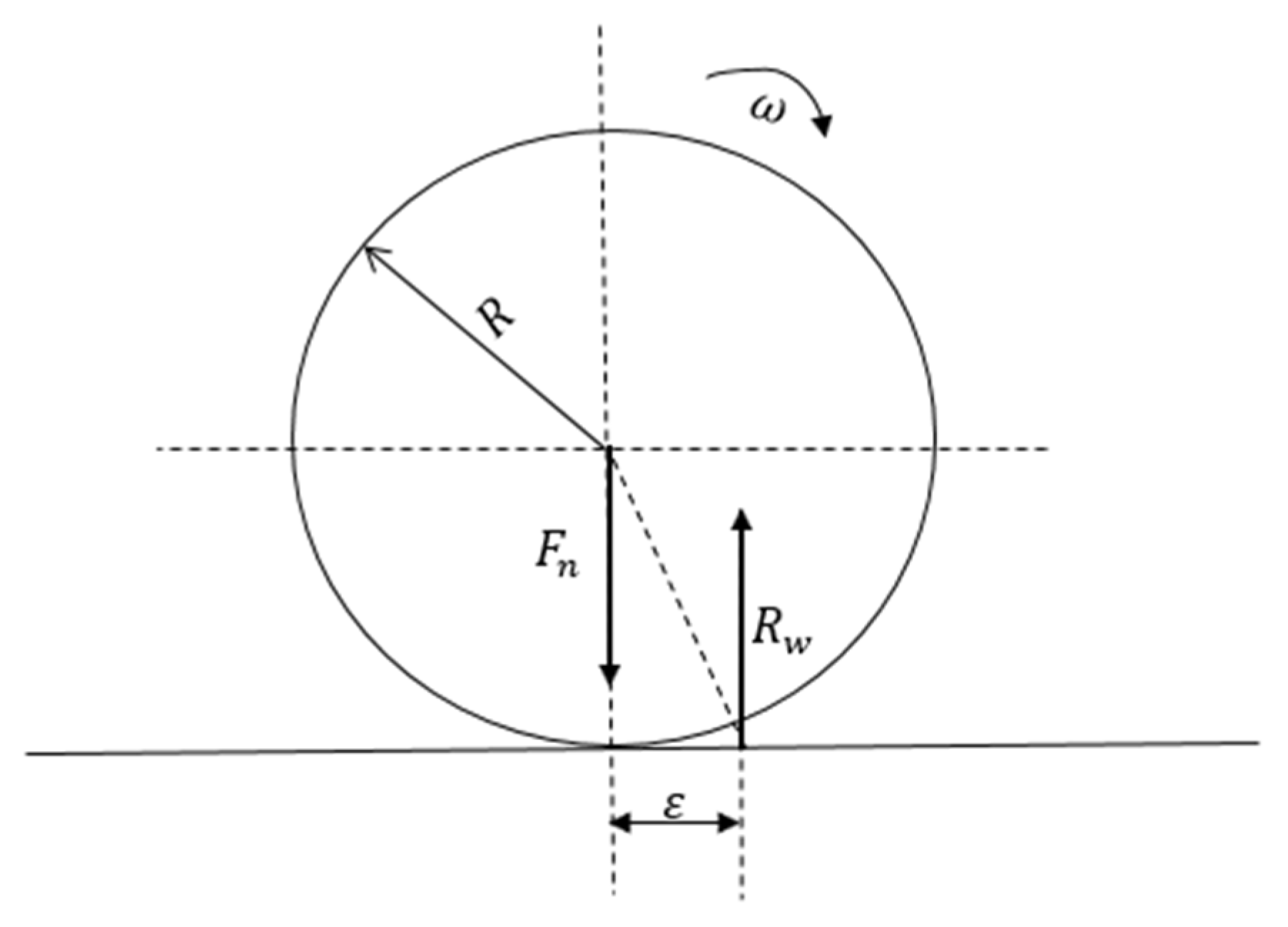
2.3. Rolling Friction

Rolling friction torque is added to the present model to study the heap formation of a soil sample. Rolling friction is a dimensionless coefficient defined as the force that resists the movement of a particle rolling on a surface [29]. In some cases, it can be taken as the angle of internal friction [30]. In this case, the granular material should have a uniform particle size, density, and moisture content. Some researchers consider the rolling friction as a coefficient with a unit of length [31]. When a spherical particle is in rotation on a surface, the contact between it and the surface generates a force $R_w$ that does not pass through the sphere’s center. The eccentricity between the direction of the force and the vertical line passing through the particle center is considered the rolling friction coefficient (Figure 3). However, it can be decomposed into two parts: a length parameter and a dimensionless parameter [22]. For non-spherical particles, according to [23,32,33], it is the eccentricity $\epsilon$ between the line of action of the normal contact force and the centroid of the particle (Figure 4).

For the study of the heap formation of spherical or circular particles, rolling friction is of particular interest to obtain good simulation results. Markauskas et al. [34] proved that if the rolling friction is ignored or set to zero, even with a maximum sliding friction coefficient, the model cannot correctly predict repose angle. Instead, it produces a lower angle of repose than the one given by the experiments. It is one reason we need to implement a rolling friction torque in contact models to study heap formation. Another primary reason is the difficulty in DEM simulations to model the real shape of the granular material. With rolling friction, the effect of the particle shape is well simulated. In fact, when a particle is rolling, energy dissipation comes mainly from its shape effect, even though a little part is due to micro-sliding, visco-elasticity, plasticity, and surface adhesion [32]. Rolling friction simulates the particle shape by opposing the rolling and dissipating the rolling energy of the particle as its natural shape would do. Thus, it is a good alternative to give us realistic results with simple particle shape by introducing a “shape like” behavior to a particle [32]. However, rolling friction torque is always resistant, while the torque induced by particle shape can either resist the movement or favor it. The particle shape’s simplicity further reduces the computer resource consumption that is very important when dealing with thousands of particles.

Ai et al. [22] classify the rolling friction models into four groups called model A, model B, model C, and model D. In this study, only models A, B, and C will be investigated.

Model A, or directional constant torque model, applies a resistant torque to both particles in contact. That torque is always against the relative rolling direction. Zhou [35] used that model to study the formation of a sand pile. According to it, the rolling resistance torque is given by:

$$T_r=-{\mu }_r{R}_r\left|F_n\right|\frac{{\omega }_{rel}}{\left|{\omega }_{rel}\right|}$$

(11)

where ${\mu }_r$ is the coefficient of rolling resistance, $R_r$ the effective rolling radius is given by Equation (12), $F_n$ is the contact normal force, and ${\omega }_{rel}$ the relative angular velocity between the particles in contact.

$$R_r=\frac{r_I{r}_J}{r_i+r_j}$$

(12)

Model B, also called the viscous model, applies a resistant torque given by:

$$T_r=-{\mu }_r{R}_r\left|F_n\right|({\omega }_i{r}_i-{\omega }_j{r}_j)$$

(13)

This rolling resistance torque is proportional to the translational velocity, as we can notice in the formula.

In model C (elastic-plastic spring-dashpot models), the rolling friction is divided into two parts: a spring torque $T_r^k$ and a viscous damping torque $T_r^d$. This model is similar to that of [36]. However, it has been modified by [22] to make it applicable to cyclic rolling cases. The elastic torque is given by:

$$\{\begin{array}{c}{T}_{r, t+\Delta t}^k= T_{r,t}^k-k_r\Delta {\theta }_r \mathrm{if} \left|T_{r, t+\Delta t}^k\right| < {\mu }_r{R}_r\left|F_n\right| \\ T_{r, t+\Delta t}^k = {\mu }_r{R}_r\left|F_n\right| \frac{T_{r,t}^k-k_r\Delta {\theta }_r}{\left|T_{r,t}^k-k_r\Delta {\theta }_r\right|} otherwise\end{array}$$

(14)

where $T_{r,t}^k$ and $T_{r, t+\Delta t}^k$ are the spring torques at time $t$ and $t+\Delta t$, $-k_r\Delta {\theta }_r$ is the incremental torque after each time step given by the multiplication of the incremental relative rotation $\Delta {\theta }_r$ the angle between the two particles and the rolling stiffness $k_r$. Here, the amplitude of the spring torque is limited by ${\mu }_r{R}_r\left|F_n\right|$ that is the torque corresponding to the total mobilization of the rolling angle. In our study, we use $k_r$ for two discs in contact as derived by Jiang et al. [36].

$$k_r=3S_n{\mu }_r^2{R}_r^2$$

The viscous damping torque $T_r^d$ is expressed as follows:

$$\{\begin{array}{c}{T}_{r, t+\Delta t}^d=-C_r\dot{{\omega }_r} \mathrm{if} \left|T_{r, t+\Delta t}^k\right|<{\mu }_r{R}_r\left|F_n\right| \\ T_{r, t+\Delta t}^k=-f{C}_r\dot{{\omega }_r} \mathrm{if} \left|T_{r, t+\Delta t}^k\right|={\mu }_r{R}_r\left|F_n\right| \end{array}$$

(15)

where $C_r$ is the rolling viscous damping coefficient expressed as the product of the critical rolling viscous damping coefficient $C_{crit}$ and the rolling viscous damping ratio ${\eta }_r$.

$$C_{crit}=2\sqrt{I_r{k}_r}$$

${\omega }_r$ is the relative angular velocity. $f$ is a binary factor that always activates the viscous damping torque if set equal to 1 or activates it only before the contact rolling torque is fully mobilized when set to 0. In our study, $f$ is set to 0. $I_r$ is the equivalent moment of inertia for the relative rotation given by:

$$I_r=\frac{1}{\frac{1}{I_i+m_i{r}_i^2}+\frac{1}{I_j+m_j{r}_j^2}}$$

where $I_i$, $m_i$ are the moment of inertia and the mass of particle i, $I_j$, $m_j$ the moment of inertia and mass of particle j.

More details about these models can be found in [22].

2.4. Numerical Model

A 2D DEM simulation is performed using a self-implemented Fortran program to study the dynamic heap formation of wet and dry soil using rolling friction models A, B, and C already described. Particles have a circular shape with a uniform radius. The 2D approach is chosen to simplify the problem. Moreover, it is computationally more efficient. This is very important when simulating a cohesive model because of its computational cost. Other researchers have adopted this approach for real problems and have found satisfactory results. These results are usually applicable to 3D systems [22]. The simulation is done in two parts.

First, the particles fall under gravity without initial velocity in a box of 0.62 m width and 1.05 m depth bordered by three walls. This aims to reduce the packing influence on the results and study different cases with different initial dispositions. The drop height H is defined as:

$$H=2n_v{d}_v$$

where $n_v$ is the number of particles in the vertical direction, and $d_v$ the distance separating two particles in that direction.

After several time steps enough to let them settle till they reach a static equilibrium with minimal kinetic energy, we proceed to the second part, which consists of moving the sidewalls outward with a constant velocity $V_{xb}$ that allows particles to move without any constraint and enter in a dynamic flow phase. The studies indicate that as long as the settling time is not too short, it will not affect the heap formation much [23]. The value of $V_{xb}$ is chosen so it does not affect the results. It is not too small to avoid contacts between the particles and the walls when they move. It is also not large to prevent the system from being disrupted. Simulations were run as trials, and using the dichotomy method, we chose $V_{xb}$ equal to 1.8 m/s. The second part of the simulation is run until the particles reach a final static equilibrium state. They reach that state before 4.315 s in all our simulations. The particle system’s behavior can then be analyzed, and different parameters of the system can be calculated throughout the flow and after the final static equilibrium. Numerous simulations are run with different dry and wet conditions to study the bulk behavior and the influence of the water content and the rolling friction model. Our simulation test setup is a good way to evaluate the dynamic behavior of liquids and granular materials in transient conditions. They incorporate the 3 critical phases: the triggering phase, the “fully-developed” flow, and the final jammed state. Furthermore, the first falling stage of the particles avoids crystal-like ordering of the discs and gives more natural initial packings.

The validity of the present model is ensured by experimenting with glass bead dynamic heap formation and its macroscopic comparison with our simulation results. The parameters of the Jumijin sand that we use in our study can be found in the literature [37]. The contact parameters between the particles and the liquid (contact angle and surface tension) are the same as in [17]. The liquid under consideration is water. The parameters used in our simulations are recorded in

Table 1. Parameters used for our numerical simulations.

Name of Variables	Symbol	Value
Particle Diameter (mm)	$\mathrm{D}$	10
Number of particles	-	3600
Particle Density (Kg/m3)	$\mathsf{\rho }$	3270
Damping Coefficient	${\mathrm{C}}_{\mathrm{n}}$	0.012
Sliding friction coefficient	$\mathsf{\mu }$	0.36
Coefficient of restitution	$\mathrm{e}$	0.96
Coefficient of rolling friction	${\mathsf{\mu }}_{\mathrm{r}}$	0.4
Rolling viscous damping ratio	${\mathsf{\eta }}_{\mathrm{r}}$	0.5
Young’s Modulus (MPa)	$\mathrm{E}$	70
Poisson Ratio	$\mathsf{\nu }$	0.3
Surface tension	$\mathsf{\gamma }$	0.073
Initial liquid volume per particle (m3)	$-$	1.4 × 10−10 to 1.4 × 10−4
Contact angle (rad)	$\mathsf{\theta }$	0
Lateral walls opening velocity (m/s)	${\mathrm{V}}_{\mathrm{xb}}$	1.8
Initial packing concentration	$\mathrm{c}$	0.88

:

3. Results and Discussions

3.1. Rolling Friction Effect on Dry Coarse Soil

Rolling friction is fundamental in the studies of granular materials heap formation. Without rolling friction, it is impossible to have a stable pile with spherical or circular particles [34]. However, our simulation pointed out that a high value of the sliding friction coefficient can cause a small pile formation with the absence of rolling friction (Figure 5c). Figure 5, Figure 6, Figure 7 and Figure 8 show the simulation results without rolling friction, with rolling friction using model A, model B, and model C, respectively, with 100 and 2500 particles. The wet particles simulations are performed using a liquid volume equal to $5\times {10}^{-6}$ ${\mathrm{m}}^3$. We notice that we have heaps similar to experimental tests only with models A and C. Without the rolling friction, we have no other mechanical force stopping the particles from rolling away. As a result, we have no significant heap and some particles run out of our visualization domain (Figure 5). The particle system’s density combined with the high sliding friction coefficient explains the small pile in Figure 5c,d. In contrast, with a low sliding friction coefficient or a small number of particles, we would have no heap formation (Figure 5a,b).

With model B, we have a small pile compared to models A and C. In this model, the torque is proportional to the relative translational velocity at the contact between two particles due to relative rotation [22]. When the particle is static, the torque is equal to zero. The system becomes equivalent to one without rolling friction. Our simulation setup involves both a pseudo-static phase till 2.22 s and a dynamic phase from 2.22 to 4 s (Figure 9). The particles are colored according to their speed. The color gradient goes from blue for static particles with a velocity equal to $0 \mathrm{m}/\mathrm{s}$ to red for particles with higher speed with a maximum velocity equal to 3.99 $\mathrm{m}/\mathrm{s}$ reached during the free-falling phase. Before the opening of the sidewalls, all particles are static. The results show that even the translational velocities caused by the particles’ collapse are not enough to have a stable pile. Therefore, model B should not be used to study granular materials involving a static phase even though a dynamic phase follows it. Thus, this model will not be investigated in the following sections.

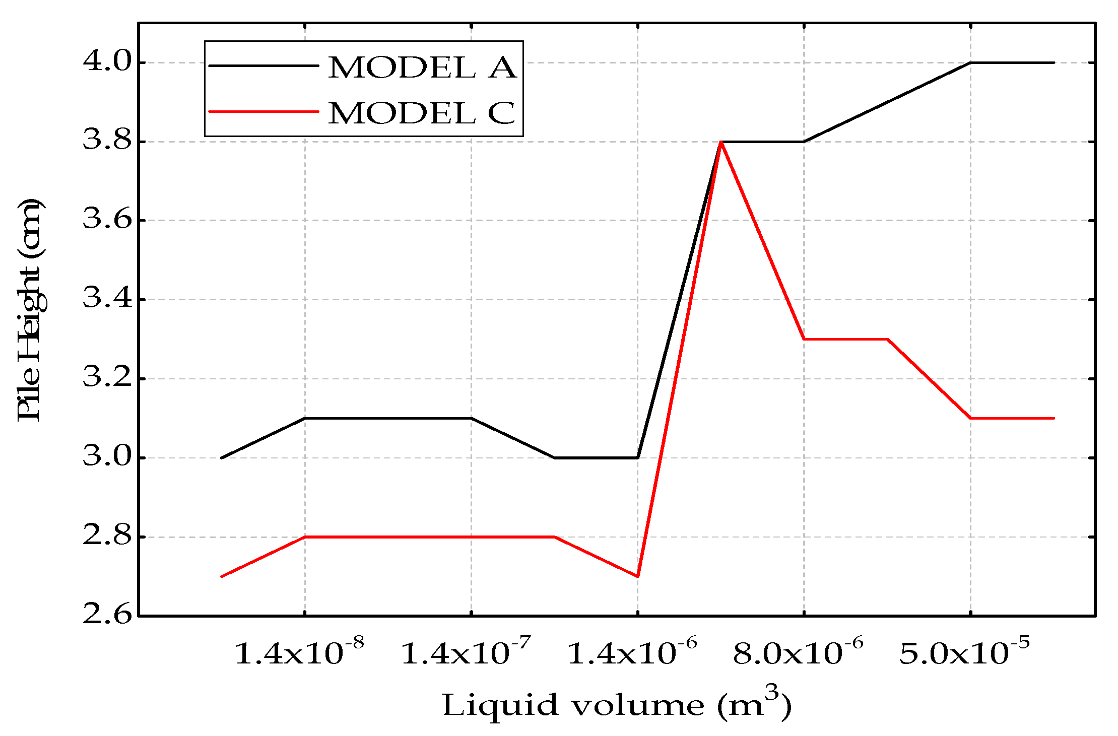
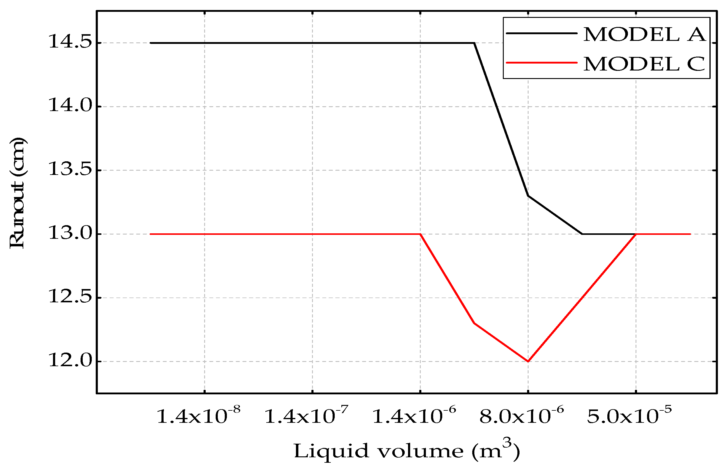
3.2. Rolling Friction Effect on Wet Coarse Soil

We performed simulations with different liquid volumes to study the system behavior and the effect of the liquid bridge volume’s variation on the stability of the particles. We considered two cases:

In case A, we follow the procedure described before. The particles fall vertically and are subject to rearrangement before opening the sidewalls. This procedure gives us slightly different initial packings depending on the liquid volume and the rolling friction model. In case B, dry conditions with no rolling friction are applied during the falling. Then, the cohesion and capillary forces are applied before the walls’ removal, after the particles are settled. In this case, we have the exact initial packings.

For monosized discs in the presence of a liquid, we have three states [38]: The pendular condition refers to the low moisture content in a packing in which liquid is retained as discrete lenticular rings at particle contacts. When the moisture content is higher, the rings will merge and form a continuous liquid network, resulting in another state called the funicular state. An increasing rise in moisture content causes the capillary state, in which the pores between particles are totally filled with liquid. In our study, 11 cases with liquid bridge volume varying from $1.4\times {10}^{-4}$ to 1.4 $\times {10}^{-10}$ ${\mathrm{m}}^3$, covering all of the three states are carried out. These states can be defined according to the liquid content, which is the mass of the liquid over the particle’s mass and varies with the initial concentration. The moisture contents corresponding to our liquid volumes vary from 6.14 $\times {10}^{-3}$ to 6140%, covering a wide range.

Table 2. The states of a particles system in presence of a liquid.

States	Liquid Content
Pendular	$0< \mathrm{M} (\%)<9.2$
Funicular	9.2 < M (%) < 26.7
Capillary	M (%) $\ge$ 26.7

gives the liquid content corresponding to the three states for a porosity equal to 0.4.

In case A, the results show that the wet particles cohesion model effect on coarse discs heap formation is minimal. This effect is mainly noticed in the particle arrangement and the energy variation rather than the heap formation. With very small amounts of liquid corresponding to a pendular state (liquid volume equal to 1.4 $\times {10}^{-10}{\mathrm{m}}^3$), the behavior of the particles is similar to the dry condition with the same final heap height for models A and C. The heap only begins to increase when the volume of liquid brings the particles into the funicular states, suggesting an increase in the cohesion and capillary forces enough to influence the bulk behavior.

With the two models, our simulations showed a different behavior on both sides of a threshold liquid content equal to $219\%$ (liquid volume equal to 5 $\times {10}^{-6}{\mathrm{m}}^3)$. With model A, from the threshold value, the pile increase with the liquid volume until the maximum asymptomatic value of 4 cm is reached. For model C, this value gives us a peak of heap equal to 3.8 cm. Then the height decreases with larger liquid volume until an asymptotic value of 3.1 cm. Figure 10 shows the pile height obtained with models A and C with different liquid volumes. The presence of asymptotic behavior for increasingly higher water contents is a common phenomenon reported in various tests with spheres or discs (column collapse, shear strength curves of unconfined radial and axial compression tests, and direct shear tests [18]).

An analysis of the variation of the pile height against the initial packing height of the particles shows that the latter is the fundamental parameter that determines the final size of the pile, as shown in Figure 11.

This hypothesis is confirmed by case B simulations. In fact, the results with case B show us a minimal difference between the heights of the heaps from one volume of liquid to another with all two models. In dense packing, the cohesion force reaches a maximum value and does not vary when increasing the liquid content. Moreover, the number of capillary bonds does not increase. The effect of increasing the volume of liquid is therefore only noticed when the sidewalls are opened. However, in this dynamic phase, with the particles’ velocity and size, and the fact that the capillary force only acts in the normal direction, this effect cannot create a noticeable variation in the pile height.

We made similar observations about the runout length, which is the horizontal distance covered by the particles after the final static equilibrium (Figure 12). Previous studies have shown that the runout length in wet conditions can be even slightly higher than the dry values because of the lubrication of the contacts [18].

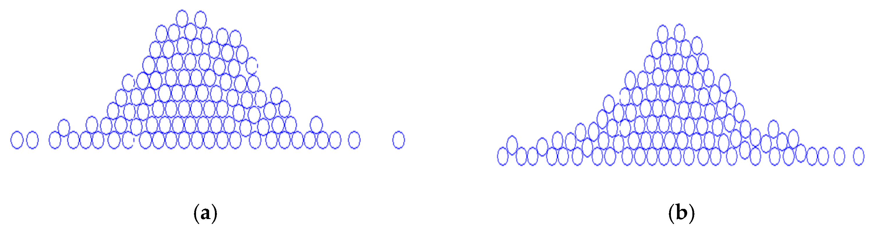
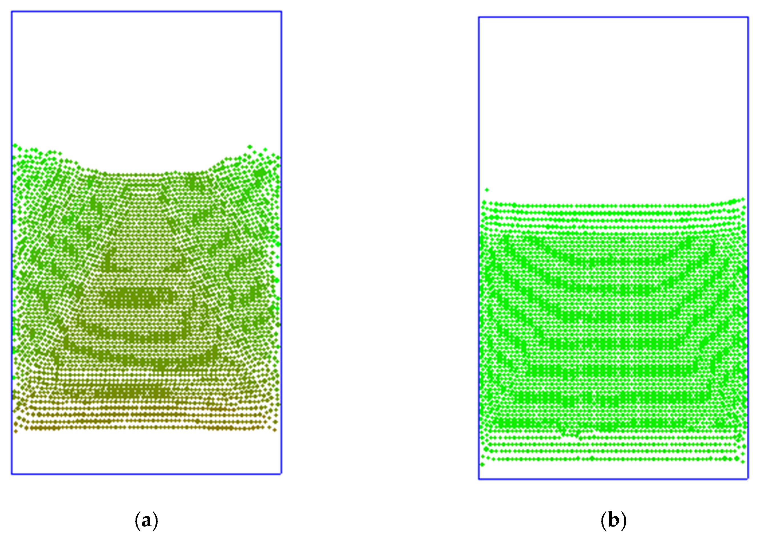
3.3. Initial Particles Packing Effect

The interaction between the particles and the lateral walls has a big influence on the initial packing of the particles. Its effect depends on the rolling friction models but also on the liquid content. In dry conditions, the particles falling phase is similar to a free fall. In that case, the proximity between the particles and the lateral walls is not close enough to create contact forces and moments. Meanwhile, with high liquid volumes with model A, we noticed friction forces that produce a “wave” configuration in the granular media, leading to different trajectories of the particles. The attraction between the particles and the sidewalls happens as soon as the liquid content reaches the threshold value of $219\%$ with model A, whereas with model C, it was not noted (Figure 13). At a particular volume of liquid, the capillary attraction force is large enough to bring particles closer to lateral walls. The result is a frictional contact force and a moment that tends to change the trajectory of the particles. To explain the difference of the behavior with models A and C, we isolated the torque produced by the interaction between the particles and the walls. Figure 14 displays the mean value of the torque, by time step, from particle-wall interactions. When we extract the part corresponding to the falling phase, we can see the difference in the amplitude of the torque for models A and C. When in contact with a wall, the relative angular velocity is equal to the particle velocity. With model C, it results in an increase of the torque, while it has no effect with model A because the relative angular velocity is normalized by its absolute value.

Model A produces a low torque depending only on the normal force and cannot resist the momentum created by the friction. In contrast, with model C, the combination of the spring and the dashpot torques is high enough to produce rolling resistance.

To study the effect of the initial particles’ arrangement during the static phase before the walls opening, we have selected and isolated the particles inside the triangle formed by the axis of the bottom wall and the lines passing through ($-$L/2,0) and (0,60D) on the one hand, and (L/2,0) and (0,60D) on the other hand (see Figure 15). Figure 16 shows the relationship between the fraction of the particles in this triangle and the final height of the wet pile in model A and C cases, respectively. The result shows that in both model A and model C cases, the height of the pile increases when that ratio, i.e., the number of particles in the triangle area decreases, regardless of the volume of liquid in the system. This means that the cohesion force is not significant enough compared to the other forces in the case of coarse discs subjected to a dynamic phase. The height of the pile depends more on the number of particles in the central triangle area than on the volume of liquid. As the number of particles in the triangle increases, this results in an increase in the concentration of the packing, the contact force chain, and the elastic potential energy. The binary cohesion force does not increase. Therefore, after the opening of the lateral walls, the repulsive force between the particles combined with the action of the gravity force decreases the height of the residual pile.

The aspect ratio is an important parameter whose study allows a better understanding of the flow dynamics. It is defined as the ratio of the initial height to the initial half-width of the packing.

$$A_a=\frac{H_i}{R_i}$$

The free fall of particles gives us an initial packing of particles that vary slightly according to the amount of liquid and the rolling resistance model.

We found out that, for our column aspect ratio $A_a$, the measured final runout radius, $R_f$, is related to the initial radius by $R_f$ = $R_i$ (1 + 2.21$A_a$) for model A and $R_f$ = $R_i$ (1 + 1.87$A_a$) for model C.

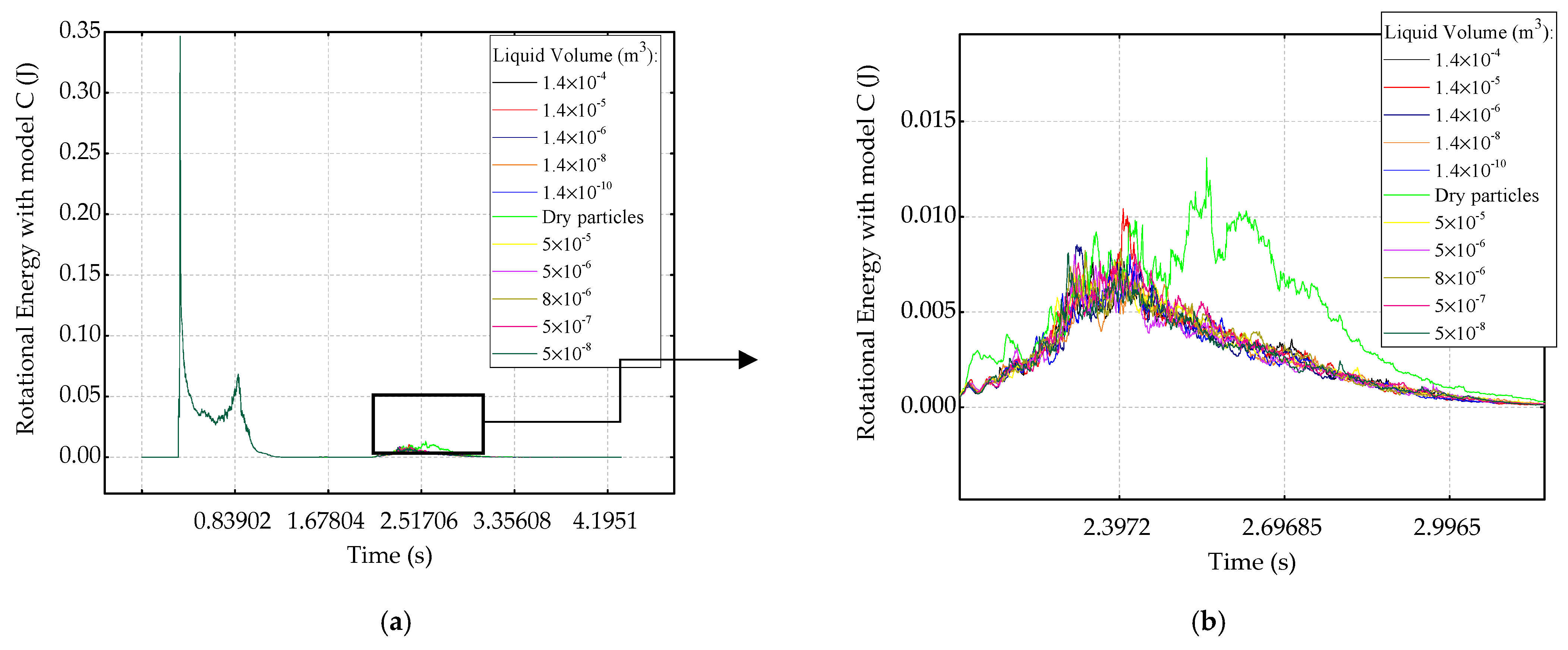
3.4. Energy Monitoring

Energy monitoring is a good way to study granular media subjected to different flow phases and their stability. We investigated the energy variation of the bulk first during the whole process of our simulation (case A). Then we recorded the energy variation from the same initial packing to point out the exact contribution of the liquid volume (case B).

All kinetic energy graph curves follow a similar pattern both under dry and wet conditions after the free fall and settling of the particles with three phases: an initial phase with almost zero energy, from 1.2 to 2.2 s, corresponding to the static phase before the opening of the sidewalls, a peak that happens right after the movement of the walls around 2.39 s, and then a return to a static state with no residual kinetic energies. The potential energy goes from a maximum value before opening the wall to a residual value when the system reaches the static equilibrium.

In case A, the kinetic energy recorded with different liquid volumes has a slight difference between the dry and wet cases. The dynamic process involves a lot of collisions and momentum lost and transfer. When the initial packing is different, it is almost impossible to have comparable kinetic energies. On the other hand, the potential energy curve interpretation clearly points out the existence of the threshold value of the liquid content equal to $219\%$ (liquid volume 5 $\times {10}^{-6}{\mathrm{m}}^3$) above which all the potential energies are greater than the potential energy of the system in dry conditions, as shown in Figure 17 and Figure 18. Only the curves for dry particles, threshold liquid volume, maximum and minimum liquid volumes, and two values above and below the threshold are displayed. The residual potential energy at the final equilibrium state also depends on the initial potential energy before removing the walls. The higher the initial potential energy, the lower the residual potential energy. This result corroborates the results found by [21], who studied the collapse of granular columns.

With case B, the kinetic energy variations become clearer. We have a clear difference between the rotational kinetic energy for the dry case and for wet cases with model C. However, with Model A, these variations are less highlighted (Figure 19 and Figure 20).

With model C, the cohesive model decreases the rotational kinetic energy, while with model A, there is only a slight decrease in kinetic energy after the peak, when the system tends toward its static state (Figure 17b). The cohesion and capillary forces only act in the normal direction by reducing the amplitude of the normal contact force. The torque produced by model A has a constant value ${\mu }_r{R}_r{F}_n$ during a time step duration and is directly linked to the normal contact force. Thus, a reduction in the value of the normal force tends to diminish the value of the torque. However, because of the disc size, the cohesion and capillary forces are small compared to the contact forces. However, in model C, only the spring rolling friction torque is limited by ${\mu }_r{R}_r\left|F_n\right|$. Of course, this results in a narrower spring rolling resistance variation range with lower maximum value. Although, added to the damping rolling resistance and combined with the fact that this rolling friction is proportional to the relative angular velocity between the particles in contact make it more efficient in reducing the kinetic energy in wet conditions than model A. The same observations were made with the potential energy graph (Figure 21 and Figure 22). In fact, we have an apparent increase in potential energy when we use the cohesive model compared to the dry conditions with model C. However, for model A, there is not always an increase of the potential energy, and in some cases, the potential energy with the dry particle simulation is greater than the one with wet particles.

Theoretically, a high residual potential energy is supposed to give a high pile. However, we noticed an arching phenomenon (Figure 23) also noted in previous studies [39], when we use model C. We call arching phenomenon the rounded shape taken by the heap instead of the usual triangular shape we expected. Despite the fact that both models have almost the same potential energy as we see in Figure 24, and the small kinetic energy noted when using model C, we often have a higher pile with model A with a difference that can reach 9 mm in case A simulations. With model C, the torque that emerges from the interaction between a particle and a wall is greater, as we see in Section 3.3. When we open the lateral walls, particles in contact with the bottom wall roll over a minimal distance. With the imbalance of the particles at the top and the action of rolling resistance proportional to the relative angular velocity, the pile shape transforms into an arc with a final height lower than the height found with model A. At the beginning of the dynamic flow phase, we have lower angular velocities and torque with model C (Figure 25). The torque increases gradually when the relative angular velocity increase. This makes it very efficient to stop the particle from rolling sideways but not sufficient to prevent the central particles at the top from falling. For model A, the torque is directly applied with a constant value high enough to keep the particles at the center in equilibrium at the top of the pile. At high liquid volume, the arching disappears.

With a comparative graph as in Figure 26, we note that model C has lower kinetic energy than model A both in dry and wet particles simulation. In both simulations, model C appears to be more suitable for reducing the system’s kinetic energy even though, in our simulation, we eliminated the dissipation by viscous damping when the spring torque reaches the limit value. This is due mainly to its ability to stop the particle circular motion when rolling on a wall, as discussed in Section 3.3. Moreover, by preventing the hysteresis phenomenon, the damping part of the torque decreases the kinetic energy. With model A, there is no damping mechanism in the friction torque. The loss of kinetic energy will only result from the frictional damping effect.

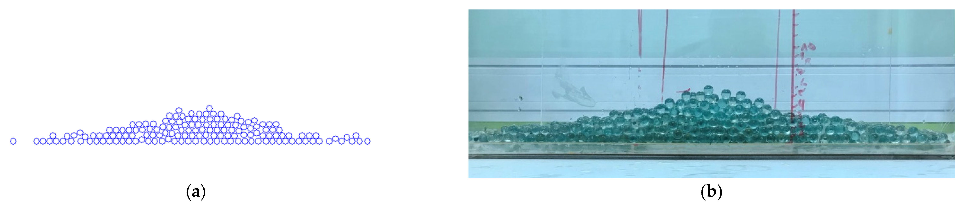
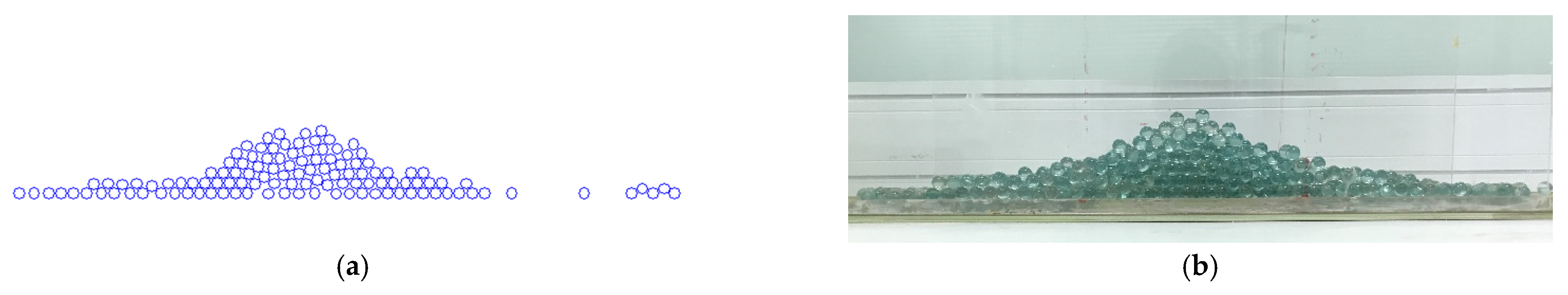
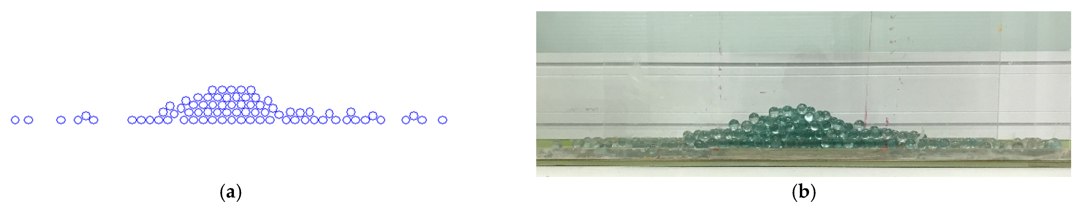
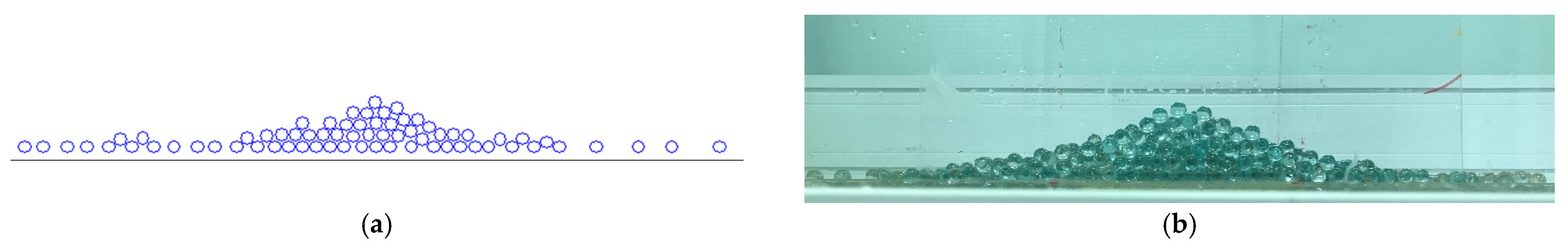
3.5. Model Validation

We performed experiments in the laboratory using glass beads for the validation of our model. Our study using a macroscopic approach of DEM, we validate our results by comparing the heaps obtained by simulation and experiment. The front and rear walls are totally fixed, and particles can only flow in the lateral direction giving a prismatic heap. To have a concordance of dimensions, we use the projection on the front wall of the result from our experiment, which can be compared with the simulation result [40,41]. This is done by taking our photos from a frontal and perpendicular point of view. For the experiment with 2400 particles, the particles are arranged in 16 × 10 × 15 inside the confining box. 16 represents the number of particles in the horizontal direction, 10 the number of particles in the vertical direction, and 15 the number of particles in the third dimension. Thus, considering the vertical plane section, we get 16 × 10 particles that we will consider for our 2D simulation. In all the experiments, the number of particles in the third dimension does not change.

We designed a device made of four vertical glass plates arranged on a horizontal one used as a bottom wall (see Figure 27 and Figure 28). The two lateral plates have central holes allowing a fifth plate to maintain the glass beads before the falling phase. Particles are first put in the upper part of the device before we remove the middle plate and let them fall in the box below and settle under gravity (Figure 27). Finally, we remove the lateral walls. For the numerical simulations, rolling friction is introduced to account for the little groove in the bottom wall of our experimental device. A calibration test was conducted to determine the rolling friction coefficient by a simple angle of repose test. The rolling friction coefficient is found equal to 0.03 after simulations were carried out to match a laboratory calibration test. Model A is used in all our simulations. The glass beads have the characteristics recorded in

Table 3. Glass beads parameters used in our numerical simulation.

Name of Variables	Symbol	Value
Particle Diameter (mm)	$\mathrm{D}$	10
Number of particles	-	From 80 to 160
Particle Density (Kg/m3)	$\mathsf{\rho }$	2500
Sliding friction coefficient	$\mathsf{\mu }$	0.26
Coefficient of restitution	$\mathrm{e}$	0.73
Coefficient of rolling friction	${\mathsf{\mu }}_{\mathrm{r}}$	0.03
Young’s Modulus (MPa)	$\mathrm{E}$	11
Poisson Ratio	$\mathsf{\nu }$	0.29
Initial packing concentration	$\mathrm{c}$	0.88

.

We determined the value of the restitution coefficient by a simple drop test, and the Young’s modulus, Poisson ratio, and viscosity coefficient between glass beads and different materials can be found in the literature.

Figure 28, Figure 29, Figure 30 and Figure 31 show the experiments and simulation results of the heap formation of glass beads with different aspect ratios in dry conditions. Figure 32, Figure 33, Figure 34 and Figure 35 show the experiments with two different packing conditions and liquid volumes. From the snapshots, we can see that a high aspect ratio generally leads to a low pile height confirming the influence of the initial potential energy on the final height of a soil heap discussed in Section 3.4. Overall, we notice that we have good similarities between the piles obtained in simulations and experiments both in wet and dry conditions. More experiments and simulations were performed with different aspect ratios, and the results are shown in Figure 36. We remark that in both the experiment and simulation, the pile height decreases when the aspect ratio increases. Therefore, the results found with the experiments are in good agreement with the simulation results.

4. Conclusions

The discrete element method has become a trustful numerical method in engineering. Its invention has allowed the numerical study of granular materials in many fields with reliable results. However, one of the major difficulties of this technique is modeling the shape of the particles. This fact explains the introduction of rolling friction to simplify the calculations and reduce computer resource consumption and make the results compliant with laboratory tests.

In this paper, the influence of rolling friction on the formation of wet and dry soil piles has been studied, and a simulation procedure has been proposed. For the validation of the method, a case of practical study was carried out. For this purpose, we used circular particles and three rolling friction models combined with Hertz–Mindlin contact force model and a modified Hertz–Mindlin–JKR model, which take into account a capillary force. The results suggest that:

Friction is important in the formation of stable heaps. Without it, it is difficult to study real matter like sand or rocks using spherical or circular particles. However, the choice of rolling friction model is essential. Simulations with model A and model C give good results in agreement with laboratory results.

The simulations with model B do not give good results because of the static phase we have in our simulation.

The final heap height and stability depend on the number of particles in the central triangle domain of the packing and decrease as this number increase.

Despite acting only in the normal direction, the wet particles contact model we used in our study increases the stability of the pile. It decreases the rotational kinetic energy and increases the potential energy with model C. However, with model A, we have a different behavior because of the torque, which directly depends on the normal force.

Moreover, compared to model A, model C demonstrates greater efficiency in decreasing the system’s kinetic energy because of its effectiveness in stopping particles rolling on a wall.

In some cases, model C has a higher residual potential energy, but model A has a higher pile because of an arching phenomenon in model C simulations which makes the pile have a circular shape.

References

1. Wu, W.-T.; Aubry, N.; Antaki, J.F.; Massoudi, M. Normal stress effects in the gravity driven flow of granular materials. Int. J. Non-Linear Mech. 2017, 92, 84–91. [Google Scholar] [CrossRef] [Green Version]
2. Richard, P.; Nicodemi, M.; Delannay, R.; Ribière, P.; Bideau, D. Slow relaxation and compaction of granular systems. Nat. Mater. 2005, 4, 121–128. [Google Scholar] [CrossRef]
3. Irazábal, J.; Salazar, F.; Oñate, E. Numerical modelling of granular materials with spherical discrete particles and the bounded rolling friction model. Application to railway ballast. Comput. Geotech. 2017, 85, 220–229. [Google Scholar] [CrossRef]
4. Cundall, P.A.; Strack, O.D.L. A discrete numerical model for granular assemblies. Géotechnique 1979, 29, 47–65. [Google Scholar] [CrossRef]
5. Babić, M.; Shen, H.H.; Shen, H.T. The stress tensor in granular shear flows of uniform, deformable disks at high solids concentrations. J. Fluid Mech. 1990, 219, 81–118. [Google Scholar] [CrossRef]
6. Babic, M. Discrete Particle Numerical Simulation of Granular Material Behavior; Clarkson University: Postdam, NY, USA, 1988. [Google Scholar]
7. Fitzpatrick, J.J.; Ahrné, L. Food powder handling and processing: Industry problems, knowledge barriers and research opportunities. Chem. Eng. Process. Process. Intensif. 2005, 44, 209–214. [Google Scholar] [CrossRef]
8. Popescu, M. Foundation Analysis and Design. Eng. Geol. 1984, 20, 269. [Google Scholar] [CrossRef]
9. Al-Hashemi, H.M.B.; Al-Amoudi, O.S.B. A review on the angle of repose of granular materials. Powder Technol. 2018, 330, 397–417. [Google Scholar] [CrossRef]
10. Rackl, M.; Grötsch, F.E.; Rusch, M.; Fottner, J. Qualitative and quantitative assessment of 3D-scanned bulk solid heap data. Powder Technol. 2017, 321, 105–118. [Google Scholar] [CrossRef]
11. Li, T.; Peng, Y.; Zhu, Z.; Zou, S.; Yin, Z. Discrete Element Method Simulations of the Inter-Particle Contact Parameters for the Mono-Sized Iron Ore Particles. Materials 2017, 10, 520. [Google Scholar] [CrossRef] [PubMed] [Green Version]
12. Hosn, R.A.; Sibille, L.; Benahmed, N.; Chareyre, B. Discrete numerical modeling of loose soil with spherical particles and interparticle rolling friction. Granul. Matter 2017, 19, 4. [Google Scholar] [CrossRef] [Green Version]
13. Phillip Grima, A.; Wilhelm Wypych, P. Discrete element simulations of granular pile formation: Method for calibrating discrete element models. Eng. Comput. 2011, 28, 314–339. [Google Scholar] [CrossRef]
14. Roessler, T.; Katterfeld, A. Scalability of Angle of Repose Tests for the Calibration of DEM Parameters; Engineers Australia: Barton, Australia, 2016. [Google Scholar]
15. Khanal, M.; Elmouttie, M.; Adhikary, D. Effects of particle shapes to achieve angle of repose and force displacement behaviour on granular assembly. Adv. Powder Technol. 2017, 28, 1972–1976. [Google Scholar] [CrossRef]
16. Nguyen, D.; Rasmuson, A.; Thalberg, K.; Niklasson Björn, I. Numerical modelling of breakage and adhesion of loose fine-particle agglomerates. Chem. Eng. Sci. 2014, 116, 91–98. [Google Scholar] [CrossRef]
17. Tsunazawa, Y.; Fujihashi, D.; Fukui, S.; Sakai, M.; Tokoro, C. Contact force model including the liquid-bridge force for wet-particle simulation using the discrete element method. Adv. Powder Technol. 2016, 27, 652–660. [Google Scholar] [CrossRef]
18. Gabrieli, F.; Artoni, R.; Santomaso, A.; Cola, S. Discrete particle simulations and experiments on the collapse of wet granular columns. Phys. Fluids 2013, 25, 103303. [Google Scholar] [CrossRef] [Green Version]
19. Gabrieli, F.; Lambert, P.; Cola, S.; Calvetti, F. Micromechanical modelling of erosion due to evaporation in a partially wet granular slope. Int. J. Numer. Anal. Methods Géoméch. 2012, 36, 918–943. [Google Scholar] [CrossRef]
20. Shoji, D.; Imamura, S.; Nakamura, M.; Noguchi, R. Angle of repose of Martian wet sand using discrete element method: Implication for the seasonal cycle of recurring slope lineae(RSL) by relative humidity. arXiv 2019, arXiv:1909.06144. [Google Scholar]
21. Staron, L.; Hinch, E.J. Study of the collapse of granular columns using two-dimensional discrete-grain simulation. J. Fluid Mech. 2005, 545, 1–27. [Google Scholar] [CrossRef] [Green Version]
22. Ai, J.; Chen, J.-F.; Rotter, J.M.; Ooi, J.Y. Assessment of rolling resistance models in discrete element simulations. Powder Technol. 2011, 206, 269–282. [Google Scholar] [CrossRef]
23. Zhou, Y.C.; Wright, B.D.; Yang, R.Y.; Xu, B.H.; Yu, A.B. Rolling friction in the dynamic simulation of sandpile formation. Phys. A Stat. Mech. Appl. 1999, 269, 536–553. [Google Scholar] [CrossRef]
24. Hertz, H. On the Contact of Rigid elastic SOLIDS and on Hardness, Chapter 6; MacMillan: New York, NY, USA, 1882. [Google Scholar]
25. Mindlin, R.D.; Deresiewicz, H. Elastic Spheres in Contact under Varying Oblique Forces. J. Appl. Mech. 1953, 20, 327–344. [Google Scholar] [CrossRef]
26. Zhou, Y.C.; Xu, B.H.; Yu, A.B.; Zulli, P. Numerical investigation of the angle of repose of monosized spheres. Phys. Rev. E 2001, 64, 021301. [Google Scholar] [CrossRef] [Green Version]
27. Israelachvili, J.N. Intermolecular and Surface Forces; Elsevier: Amsterdam, The Netherlands, 2011. [Google Scholar]
28. Muguruma, Y.; Tanaka, T.; Tsuji, Y. Numerical simulation of particulate flow with liquid bridge between particles (simulation of centrifugal tumbling granulator). Powder Technol. 2000, 109, 49–57. [Google Scholar] [CrossRef]
29. Peck, W.G. Elements of Mechanics: For the Use of Colleges, Academies, and High Schools; A.S. Barnes & Burr: New York, NY, USA, 1859. [Google Scholar]
30. Nelson, E. Measurement of the Repose Angle of aTablet Granulation*. J. Am. Pharm. Assoc. 1955, 44, 435–437. [Google Scholar] [CrossRef]
31. Rao, C.L.; Lakshminarasimhan, J.; Sethuraman, R.; Sivakumar, S.M. Engineering Mechanics: Statics and Dynamics; PHI Learning Pvt. Ltd.: Delhi, India, 2003. [Google Scholar]
32. Wensrich, C.; Katterfeld, A. Rolling friction as a technique for modelling particle shape in DEM. Powder Technol. 2012, 217, 409–417. [Google Scholar] [CrossRef]
33. Zhu, H.; Yu, A. A theoretical analysis of the force models in discrete element method. Powder Technol. 2006, 161, 122–129. [Google Scholar] [CrossRef]
34. Markauskas, D.; Kačianauskas, R. Investigation of rice grain flow by multi-sphere particle model with rolling resistance. Granul. Matter 2010, 13, 143–148. [Google Scholar] [CrossRef]
35. Zhou, Y.; Xu, B.; Yu, A.; Zulli, P. An experimental and numerical study of the angle of repose of coarse spheres. Powder Technol. 2002, 125, 45–54. [Google Scholar] [CrossRef]
36. Jiang, M.; Yu, H.-S.; Harris, D. A novel discrete model for granular material incorporating rolling resistance. Comput. Geotech. 2005, 32, 340–357. [Google Scholar] [CrossRef]
37. Jang, G.; Lee, S.; Lee, K.-J. Discrete element method for the characterization of soil properties in Plate-Sinkage tests. J. Mech. Sci. Technol. 2016, 30, 2743–2751. [Google Scholar] [CrossRef]
38. Yang, R.Y.; Zou, R.P.; Yu, A.B. Numerical study of the packing of wet coarse uniform spheres. AIChE J. 2003, 49, 1656–1666. [Google Scholar] [CrossRef]
39. Lube, G.; Huppert, H.E.; Sparks, R.S.J.; Hallworth, M.A. Axisymmetric collapses of granular columns. J. Fluid Mech. 2004, 508, 175–199. [Google Scholar] [CrossRef] [Green Version]
40. Li, Z.; Wang, Y.-H.; Li, X.; Yuan, Q. Validation of discrete element method by simulating a 2D assembly of randomly packed elliptical rods. Acta Geotech. 2017, 12, 541–557. [Google Scholar] [CrossRef]
41. Mack, S.; Langston, P.; Webb, C.; York, T. Experimental validation of polyhedral discrete element model. Powder Technol. 2011, 214, 431–442. [Google Scholar] [CrossRef]
Figure 1. Forces acting on particle i during contact.
Applsci 11 06043 g001
Figure 2. Contact parameters: The contact radius a and the normal and tangential overlap δ n and δ t .
Applsci 11 06043 g002
Figure 3. Rolling friction mechanism on a circular particle.
Applsci 11 06043 g003
Figure 4. Forces acting on particle i during contact.
Applsci 11 06043 g004
Figure 5. Dry (a,c) and wet (b,d) coarse soil heap formation without rolling friction torque with 100 particles (a,b) and 2500 particles (c,d).
Applsci 11 06043 g005
Figure 6. Dry (a,c) and wet (b,d) coarse soil heap formation with Model A with 100 particles (a,b) and 2500 particles (c,d).
Applsci 11 06043 g006
Figure 7. Dry (a,c) and wet (b,d) coarse soil heap formation with Model B with 100 particles (a,b) and 2500 particles (c,d).
Applsci 11 06043 g007
Figure 8. Dry (a,c) and wet (b,d) coarse soil heap formation with Model C with 100 particles (a,b) and 2500 particles (c,d).
Applsci 11 06043 g008aApplsci 11 06043 g008b
Figure 9. Simulation phases with 2500 particles: (a) the initial phase after the collision of the particles with the bottom wall. In (b), particles reach a static equilibrium before the opening of the walls. (c) particles enter the dynamic phase. Finally, in (d), the particles flow to reach the final static equilibrium state shown in Figure 7c.
Applsci 11 06043 g009
Figure 10. Pile height variation with the liquid volume with models A and C. Both models have an asymptotic behavior at high liquid volumes. However, Model C reaches that asymptotic value after it reaches a maximum value.
Applsci 11 06043 g010
Figure 11. Initial and final pile height variation with the liquid volumes with models A (a) and C (b).
Applsci 11 06043 g011
Figure 12. Runout length variation with the liquid volumes with models A and C.
Applsci 11 06043 g012
Figure 13. Friction forces between the lateral walls and the particles with models A (a) and C (b). We notice there is no “waving” phenomenon with model C.
Applsci 11 06043 g013
Figure 14. (a) Mean torque between the lateral walls and the particles with models A and C. In (b), we highlighted the part of the curves in the dotted blue square corresponding to the initial falling phase.
Applsci 11 06043 g014
Figure 15. Triangle area. The pile height increases when the number of particles in this area decreases.
Applsci 11 06043 g015
Figure 16. Pile height against the fraction of the packing inside the central triangle with model A (a) and C (b).
Applsci 11 06043 g016
Figure 17. Variation of the potential energy around the threshold value in case A with Model A (a). In (b), we highlight the residual potential energy after the final static equilibrium.
Applsci 11 06043 g017
Figure 18. Variation of the potential energy around the threshold value in case A with Model C. In (a), we have the variation of the potential energy during the whole simulation. In (b), we highlight the residual potential energy after the final static equilibrium.
Applsci 11 06043 g018
Figure 19. Rotational kinetic energy in case B with model A (a). In (b), we highlight the part of the curve corresponding to the flow after the opening of the walls.
Applsci 11 06043 g019
Figure 20. Rotational kinetic energy in case B with model C (a). In (b), we highlight the part of the curve corresponding to the flow after the opening of the walls.
Applsci 11 06043 g020
Figure 21. Potential energy for dry and wet particles in case B simulations with model A. (a): the potential energy corresponding to the flow after the opening of the walls. In (b) we highlight the residual potential energy after the final static equilibrium.
Applsci 11 06043 g021
Figure 22. Potential energy for dry and wet particles in case B simulations with model C. In (a) we have the potential energy corresponding to the flow after the opening of the walls. In (b) we highlight the residual potential energy after the final static equilibrium.
Applsci 11 06043 g022
Figure 23. Arching phenomenon when using model C (b) (liquid volume 1.4 × 10 6 m 3 ). We notice that model A (a) has a larger pile base in the wet particle simulation and a higher pile. Model C produces a smaller runout and greater potential energy, but the arching phenomenon decreases the pile height.
Applsci 11 06043 g023
Figure 24. Comparative potential energy for dry (a) and wet (b) particles in case B simulations after removing the walls. The wet particles simulation was done with a liquid volume equal to 5 × 10 6 m 3 .
Applsci 11 06043 g024
Figure 25. Mean angular velocity (a) and torque (b) for dry particles in case B simulations.
Applsci 11 06043 g025
Figure 26. Comparative rotational kinetic energy for dry (a) and wet (b) particles in case B simulations (liquid volume 5 × 10 6   m 3 ).
Applsci 11 06043 g026
Figure 27. Glass beads initial packing in experiment (a) and simulation (b).
Applsci 11 06043 g027
Figure 28. Simulation (a) and experiment (b) results with 16 × 10 particles in the cross-section.
Applsci 11 06043 g028
Figure 29. Simulation (a) and experiment (b) results with 9 × 13 particles in the cross-section.
Applsci 11 06043 g029
Figure 30. Simulation (a) and experiment (b) results with 16 × 8 particles in the cross-section.
Applsci 11 06043 g030
Figure 31. Simulation (a) and experiment (b) results with 16 × 5 particles in the cross-section.
Applsci 11 06043 g031
Figure 32. Simulation (a) and experiment (b) results with 16 × 5 wet particles in the cross-section (liquid volume 1.4 × 10 6   m 3 ).
Applsci 11 06043 g032
Figure 33. Simulation (a) and experiment (b) results with 16 × 5 wet particles in the cross-section (liquid volume 5.6 × 10 6   m 3 ).
Applsci 11 06043 g033
Figure 34. Simulation (a) and experiment (b) results with 16 × 8 wet particles in the cross-section (liquid volume 1.4 × 10 6   m 3 ).
Applsci 11 06043 g034
Figure 35. Simulation (a) and experiment (b) results with 16 × 8 wet particles in the cross-section (liquid volume 5 × 10 6   m 3 ).
Applsci 11 06043 g035
Figure 36. Pile height obtained with experiment and simulation versus the packing aspect ratio.
Applsci 11 06043 g036