Automatic Wheels and Camera Calibration for Monocular and Differential Mobile Robots

Abstract

Mobile robotic systems are highly relevant today in various fields, both in an industrial environment and in terms of their applications in medicine. After assembling the robot, components such as the camera and wheels need to be calibrated. This requires human participation and depends on human factors. The article describes the approach to fully automatic calibration of a robot’s camera and wheels with a subsequent calibration refinement during the operation. It consists of placing the robot in an inaccurate position, but in a pre-marked area, and using data from the camera, information about the environment configuration, as well as the ability to move, in order to perform calibration without external observers or human participation. There are two stages in this process: the camera and the wheel calibrations. The camera calibration collects the necessary set of images by automatically moving the robot in front of the fiducial markers template, and then moving it on the marked floor, assessing its trajectory curvature. Upon calibration completion, the robot automatically moves to the area of its normal operation and it is proposed to refine the calibration during its operation without blocking its work. The suggested approach was experimentally tested on the Duckietown project base. Based on test results, the approach proved to be comparable to manual calibrations and is capable of replacing a human for this task.

1. Introduction

Modern robotic systems cover a huge number of different areas, including autonomous mobile robots. Applications for such devices include manufacturing, logistics, as well as medicine. Modern medicine begins to widely use automated mobile robots, which significantly increases the quality of services provided and the level of development in this area.

The same modern mobile systems can be operated under the control of methods that rely on classical models, computer vision algorithms, and artificial intelligence technologies. Moreover, at some point in the future, these approaches can be combined to achieve the better result. Adaptive algorithms can take into account the specificity of the environment or a mobile robot in the course of their work, but even for them, it is important to know the initial configuration and features of the robot. Thus, regardless of the approach used, the task of obtaining a first approximation of properties unique to each robot remains necessary.

The paper considers approaches to calibrate mobile systems with monocular cameras, but the concept can be extended to binocular cameras as well.

Calibrating robots is an essential step that must be completed before putting it in operation. As a rule, this is required in order to take into account the robot’s unique features, design errors and take into consideration the systematic error when processing data from robot sensors or when using its actuators. The Duckietown project is a network of miniature roads similar to automobile roads, an environment in the form of road signs, traffic lights and other things, road markings, as well as the robots themselves. It is designed for research in the field of autonomous vehicles and is well suited for the educational process. Each robot has one monocular camera as the only sensor and a differential drive.

Thus, before using the robot, its camera and wheels need to be calibrated. However, this process must be repeated for any physical changes affecting the wheels or cameras, e.g., changing the focal length or replacing the wheel motor, which is accompanied by wheel removal. From the training point of view, the calibration process can be useful, but with its regular use, especially with a large number of robots in the laboratory, it requires a large amount of time from humans, since each stage requires the direct participation of a person. Moreover, this person should be familiar with the calibration process in advance, which further complicates this task. Automation of such a routine operation would accelerate the robot preparation and in the future would provide independent control of the robot for its calibration accuracy with further automatic self-correction.

According to the most common approach for camera calibration [1], which is implemented in openCV, this process consists of two parts: calculating intrinsic camera characteristics and rotation and removing distortion. The first step begins with the formula.

$$s{m}^{\prime }=A\left[R\right|t]M^{\prime }$$

$$s\left[\begin{array}{c}u\\ v\\ 1\end{array}\right]=\left[\begin{array}{ccc}{f}_x& 0& c_x\\ 0& f_y& c_y\\ 0& 0& 1\end{array}\right]\left[\begin{array}{cccc}{r}_{11}& r_{12}& r_{13}& t_1\\ r_{21}& r_{22}& r_{23}& t_2\\ r_{31}& r_{32}& r_{33}& t_3\end{array}\right]\left[\begin{array}{c}X\\ Y\\ Z\\ 1\end{array}\right]$$

where

• $(X,Y,Z)$ are the coordinates of a 3D point in the world space;
• $(u,v)$ are the coordinates of the projection point in pixels;
• s is a scale factor;
• A is a camera matrix, or a matrix of intrinsic parameters;
• $\left[R\right|t]$ extrinsic parameters, where R is a rotation matrix and t-translation;
• $(c_x,c_y)$ is a principal point that is usually in the image center;
• $f_x,f_y$ are the focal lengths expressed in pixel units.

In the original paper, $A\left[R\right|t]$ is called a homography. Looking at the system of equations $sm=HM$, it is obvious that it requires three feature points in one image to calculate the matrix of homography. The real coordinates of these features in the real world should be known. In openCV, there is a function that takes the coordinates of points in the real world and the coordinates of their projections on the camera frame to calculate matrices A and $\left[R\right|t]$. At least three images with different views of features are required to calculate all unknown variables in matrix A.

In the second step, the distortion coefficients are calculated. They come from the system of equations

$$\left[\begin{array}{c}u\\ v\end{array}\right]=\left[\begin{array}{c}{f}_x{x}^{″}+c_x\\ f_y{y}^{″}+c_y\end{array}\right]$$

where

$$\left[\begin{array}{c}{x}^{″}\\ y^{″}\end{array}\right]=\left[\begin{array}{c}{x}^{\prime }\frac{1+k_1{r}^2+k_2{r}^4+k_3{r}^6}{1+k_4{r}^2+k_5{r}^4+k_6{r}^6}+2p_1{x}^{\prime }{y}^{\prime }+p_2(r^2+2x^{\prime 2})+s_1{r}^2+s_2{r}^4\\ y^{\prime }\frac{1+k_1{r}^2+k_2{r}^4+k_3{r}^6}{1+k_4{r}^2+k_5{r}^4+k_6{r}^6}+p_1(r^2+2y^{\prime 2})+2p_2{x}^{\prime }{y}^{\prime }+s_3{r}^2+s_4{r}^4\end{array}\right]$$

with

$$r^2=x^{\prime 2}+y^{\prime 2}$$

and

$$\left[\begin{array}{c}{x}^{\prime }\\ y^{\prime }\end{array}\right]=\left[\begin{array}{c}{X}_c/Z_c\\ Y_c/Z_c\end{array}\right]$$

In these formulas, variables k${}_1$…k${}_6$ and s${}_1$…s${}_4$ are unknown. The authors do not suggest the minimum number of images and points that are required to calculate these variables. At least five 2D points are required to calculate 10 variables. According to the previous step, the homography requires three images with three points, so this step does not require extra features or images.

In general, these two steps are repeated iteratively and the result converges to the real characteristics of the camera. Generally, more than three points and three images are taken. Extra points are processed with the least squares method, which allows the noise error to be decreased. The question of how many features are enough for the least squares method remains open.

The structure of the paper is the following. Section 2 presents the main theory and reviews the analogues; the suggested calibration process is described in Section 3; the accuracy evaluation of the process is presented in Section 4; Section 5 demonstrates the modifications of the suggested method, which help to improve accuracy; the ideas for the future work and the conclusion are described in Section 6 and Section 7, respectively.

2. Analogues Overview

The problem of camera self-calibration has been researched for more than thirty years [2]. The solution comes from regular camera calibration when intrinsic and extrinsic camera parameters should be calculated. In regular calibration processes, it is required to take several pictures of an object with known overall dimensions and calculate the camera’s focal length and parameters that reduce distortion. The process of such a calibration is well known [1] and implemented, e.g., in OpenCV. For self-calibration, a similar approach can be followed. It is possible to calculate the camera parameters automatically by taking independent pictures during the camera movement. The key problem is to distinguish truly independent pictures.

The second part of the problem under review is the wheel calibration. This calibration is required due to physical disadvantages of wheel motors. Phenomena such as friction, energy loss, and electromagnetic interference of a particular robot may influence wheel motors in different ways. Therefore, the coefficients of amperage for each wheel motor need to be calculated.

2.1. Existing Calibration Methods

The paper [3] presents an approach to the camera calibration using MEMS-sensors. The idea is to capture data both from the camera and the gyroscope independently. The authors suggest to calculate the pattern and speed of robot motion using an uncalibrated camera and gyro. Then, they use the grid search method to calculate the correlation between the motion captured using these sensors. Using the least squares method, they estimate the camera focal length and the offset between the camera and the gyro. The disadvantage of such a method is that it works in a one- or two-dimensional space according to the nature of the grid search method. The findings show that the focal length can be calculated accurately with the described method in 2D if the SIFT or ORB feature detector is applied for camera frames.

The camera self-calibration for structure from motion was discovered in [4]. In general, this approach also requires feature detection on a camera frame. Due to nonlinearities of calibration parameter estimations, the Sum of Gaussian filter is used to divide the whole nonlinear range of variations into small almost-linear pieces. Further, the authors describe the approach called the Sum of Gaussians. This approach uses several linear filters to cover all almost-linear hypotheses. After that, the authors prune these Gaussians to reduce filters to simple EKF in several steps so the complexity is reduced. Experimental results show that after 150–200 s of work the camera parameters are estimated close to offline calibration parameters. The deviation is not greater than 4%.

The disadvantage of such an approach is the algorithmic complexity, since it contains several Kalman filters, and computational time depends on the number of features detected in a frame. In addition, the described method contains a loop closing component, which also requires computational resources.

In [5], the authors track the wheeled mobile robot using an uncalibrated camera. They claim that even manual calibration might be not perfect, and therefore they describe an approach to track the robot’s movement using a camera with unknown calibration parameters. The dynamic and kinematic control models were formulated for this robot. The results show that the developed “global asymptotic position/orientation tracking controller for a wheeled mobile robot” eliminates the need for integrating the nonlinear kinematic model to achieve its cartesian position.

The authors of [6] suggest an approach for automatic extrinsic calibration of multiple cameras without placing any patterns into the environment beforehand. The robot was placed in a natural environment and carried out a set of programmed movements, including a full horizontal rotation, and captured a synchronized image sequence from each camera. The sequences were processed individually with a monocular visual SLAM algorithm. The well known SLAM techniques were applied to build monocular feature maps as the robot made controlled movements. The maps were then matched and aligned in 3D using invariant descriptors and RANSAC to determine the correct correspondences. Then, the final joint bundle adjustment was used to refine estimates and take into account all the features data. The experiments showed that for the three cameras with a 640 × 480 resolution, the images with over 80° field of view achieved 0.1° of angular error.

The disadvantage of this method, as authors claim, is its inability to work with MonoSLAM and a single camera without an intrinsic camera calibration.

An interesting approach for calibration of extrinsic and odometric parameters for a differential drive robot can be found in [7]. According to this method, the robots should not move along a specified trajectory and, moreover, it is possible to evaluate calibration parameters of the recorded data. The common idea of this method is based on considering a simultaneous calibration as a maximum-likelihood problem.

The main disadvantage of this method applied to the problem, formulated in the introduction, is that the authors do not consider calibration of intrinsic parameters of a camera.

The authors of [8] present a method of simultaneous localization and odometry calibration through filtration. There are two filtration steps in calculating systematic and nonsystematic components, and both of them use a Kalman filter. The authors show that the accuracy of the systematic error calculation is high (the difference is about 1% per 30 m of movement) and they can estimate the nonsystematic error with a relative error of 90%.

Unfortunately, this method cannot be applied without a localization step, which makes it impossible to apply to the problem addressed in this paper.

A new odometry model and its calibration techniques are presented in [9]. The authors use the Gauss–Newton based nonlinear least square method for the calibration of odometry parameters. Furthermore, they use Kalman filtration to increase the accuracy. They provide some recommendations as well for tuning the weights in the Gauss–Newton method and Kalman filter. As a result, it is shown that the GN-KF method (as the authors call it) brings almost 50% lower error of odometry position and orientation than the ordinary model calibration.

The authors admit that the correct calibration can be achieved only through the long measurement scenario to reduce the effect of initial state uncertainty.

2.2. Results of Overview

All considered analogues used either SLAM algorithms or the structure from motion approach to calculate intrinsic and extrinsic parameters of a camera on a bot. In addition, most of the works rely on the fact that the wheels are already calibrated. Only the authors of [5] claim that no calibration at all is required, but actually they do not calculate the calibration parameters, and control the robot with uncalibrated sensors. Since Duckiebot has limited resources, the idea to run SLAM algorithm in real time is not considered. Thus, the idea of calibration in this paper is based on observing calibration patterns that are placed in the neighbourhood of the robot.

The solution to separate the process of camera calibration from the wheel calibration is reasonable. It is possible to calibrate the camera taking several pictures of calibration patterns. The process of taking these pictures can be automatic—the robot may rotate observing calibration patterns around and taking as many pictures as it needs. For instance, it is possible to put two calibration boards near the robot’s initial position and make it rotate. Since the robot’s wheels were not calibrated, the rotation is not expected to be perfect, but it is enough to calibrate a camera. After taking several independent pictures of a calibration pattern, the calibration process can be performed using the openCV library.

After calibrating the camera, the robot should continue rotating to find calibration patterns for the wheels. When the camera is calibrated, it is possible to apply techniques that are similar to the process of visual odometry. The main advantage of the suggested method is its autonomy. The method makes it possible to achieve a calibration with a comparable accuracy without any human participation in the calibration process. As a result of the calibration, coefficient k is calculated for the wheels, and camera matrix K (which includes the focal length, the optical center, and the skew coefficient) and distortion coefficients D are calculated for the camera.

3. Calibration Process

3.1. Start Preset

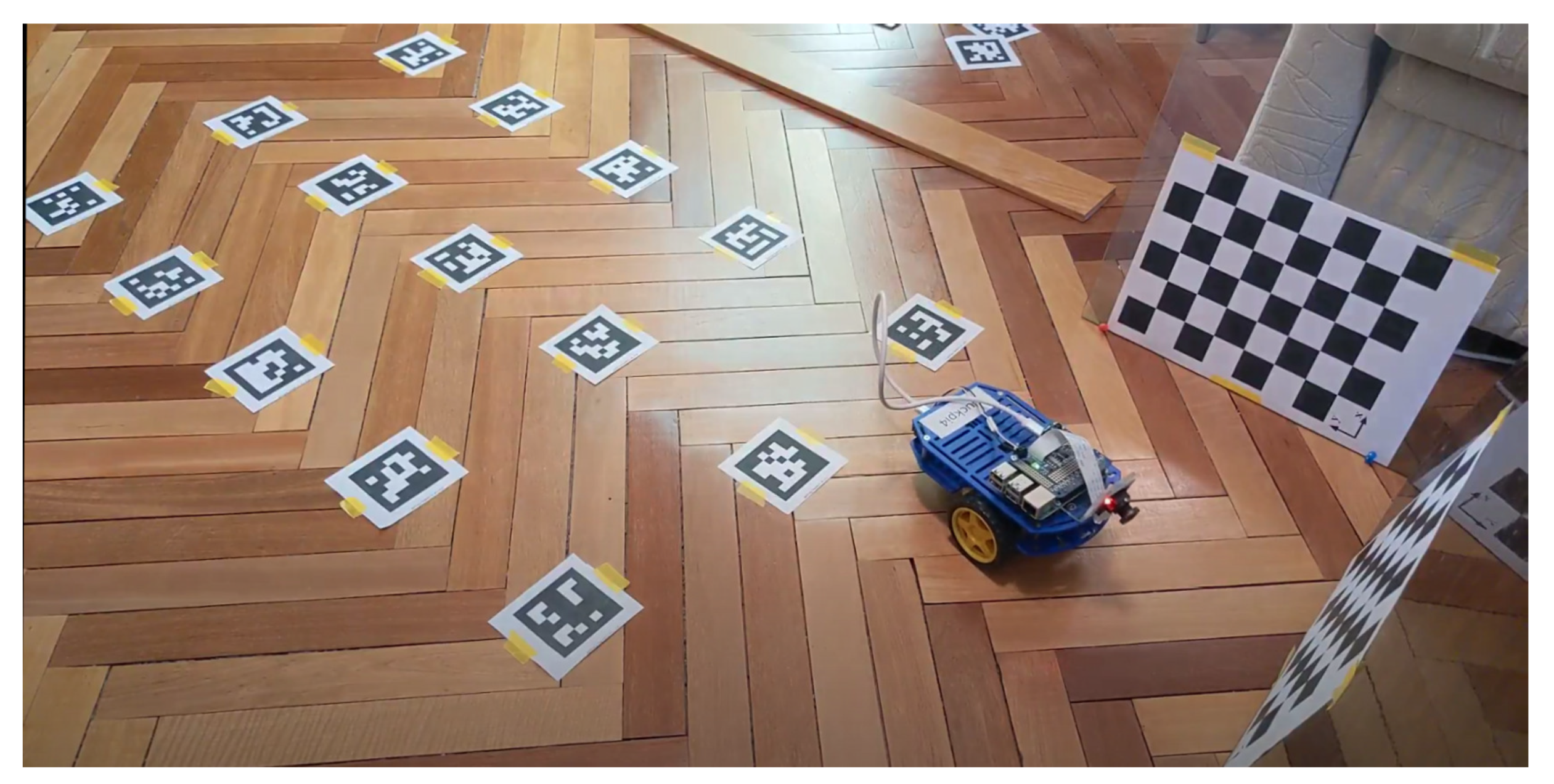
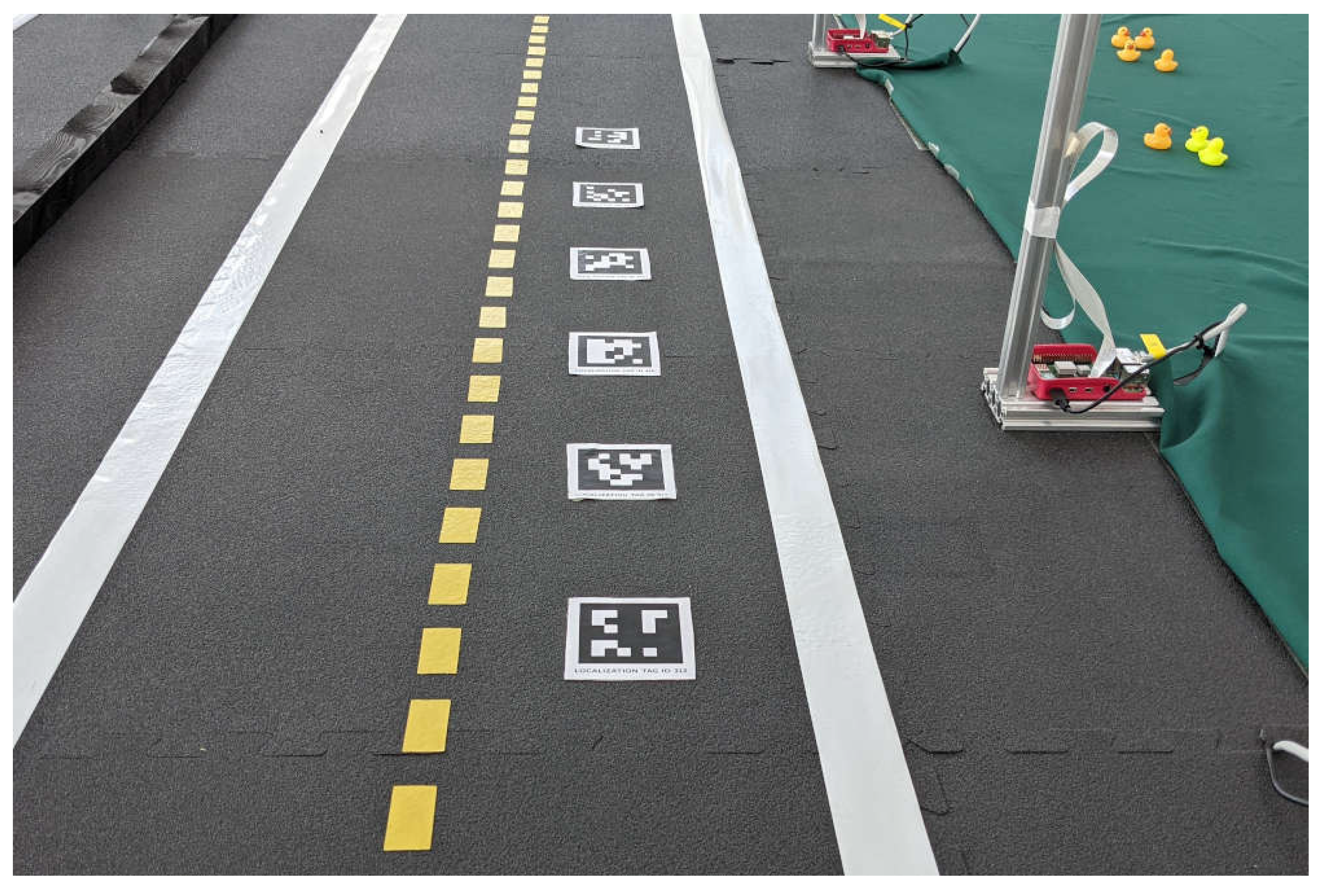
The initial position of the robot is a part of the floor with chessboards in front, where the robot is located from the very beginning, on which its camera is directed and the floorsurface is marked with aruco markers on the other side of it. An example of the initial position is illustrated in Figure 1.

There can be any number of chessboards, determined by the amount of free space around the robot. To a greater extent, the accuracy of calibration is affected by the frames with different positions of the boards, e.g., two boards located at different distances from the robot and at different angles. It is important that they are located in a semicircle and directed approximately towards the robot. Additionally, their sizes should fully fit in the camera’s field of view. The size and type of all the boards around the robot must be the same [10].

Markers should be oriented towards the chessboards and begin as close to the robot as possible. The distance between the markers depends on camera’s resolution, as well as its height and angle of inclination, but it must be such that at least three recognizable markers can simultaneously be in the frame. For Duckiebot-based experiments, the distance between the markers was set as 15 cm with a marker size of 6.5 cm. It is important to note that the distance between the markers may not be very precise 15 cm. The calibration algorithm does not take into account the relative position of the markers against each other; however, the orientation of all markers must be strictly the same. The measurement accuracy depends to a large extent on this. In addition, the algorithm assumes that the markers are oriented towards the chessboards.

The robot needs to be placed in front of the chessboards approximately in the center of the semicircle around which the chessboards are located. The exact position of the robot is not important, but initially there should be a specific board in the robot’s field of view. It can be any of the boards, but later this information needs to be provided to the camera calibration script. To eliminate the statistical error and use images from the camera taken at different distances, at least two chessboards need to be used. Since the wheel calibration validation algorithm for this robot assumes deviations of no more than 10 cm by 2 m [11], and the accuracy of the error in determining the markers position does not exceed 1 cm, it is enough for the robot to drive at least 1/3 of the test distance during calibration, which is sufficient to detect the deflection of the robot.

3.2. Camera Calibration

In fact, the camera calibration implies that the robot is rotating around its axis and taking pictures of all the viewable chessboards in turn. In this case, the ability to make several “passes” during the shooting process should be provided for, to control which of the boards the robot is currently observing and in which direction it should turn.

As a result, the algorithm can be represented as a sequence of actions: “get a frame from the camera” and “turn”. The important points to consider are:

• Which board is currently being viewed;.
• Which direction to turn;
• When to stop;
• What to do if the chessboard is not found in the picture.

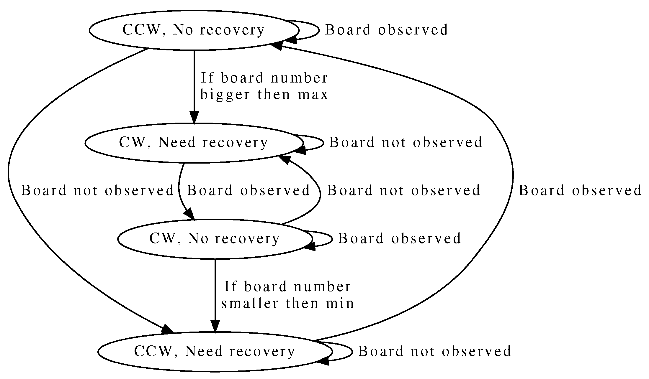
Thus, it was decided to represent the robot’s state during the camera calibration with the following set of values.

• The number of the board being observed (the boards are numbered starting from 0 counterclockwise). The initial value is determined by the robot’s position;
• The direction of the robot’s rotation. The initial value can be arbitrary; for definiteness, it is assumed to be clockwise;
• Is there a chessboard in the frame? The initial value is “true”, since the initial position of the robot suggests that the board is in the camera’s field of view;
• Is the robot in recovery mode? The recovery mode refers to a situation where the robot does not observe the chessboard, but knows where to move in order to find it. This can be either in a situation of transition from board to board or when the robot has turned so that it is not already observing the extreme board.

The algorithm of transition from state to state algorithm is visualized in Figure 2.

The robot’s rotation is performed by giving appropriate commands to its wheels. Since the wheels of the robot are not supposed to be calibrated at a given moment, it is impossible to apply speed V to the left wheel or V to the right wheel and be sure that the robot will rotate relative to its center. Therefore, it was decided to give commands only to one of the wheels. This ensures that the robot rotates relative to the point of contact of the second wheel with the floor surface. To make the image from the camera sharp, the robot moves in small steps. To do this, the minimum speed possible for the robot to move for a certain quantum of time (0.1 s) is fed to the wheel, and after that the robot stops, and only after that receives an image.

The final algorithm comprises the following sequence of actions:

• Obtain frame from the camera;
• Find a chessboard on the camera frame;
• Save information about board corners found in the image;
• Determine the direction of rotation according to the schedule;
• Make a step;
• Either repeat the steps described above, or complete the data collection and proceed with the camera calibration using OpenCV.

3.3. Moving to Wheel Calibration

After calibrating the camera, it is possible to proceed to the wheel calibration. To do this, the robot must turn to the floor space marked by aruco markers and proceed to calibration. In order for this transition to be the most general, not tied to the robot’s position in which it stayed at the end of the camera calibration, no assumptions are made about the exact orientation of the robot at this stage. In fact, the robot now only needs to turn so that it is aimed at the markers. The exact orientation with respect to the markers also does not matter at this step, but it is not advisable for the robot to be turned towards them at a large angle—such an assumption will force the marked area to be excessively wide.

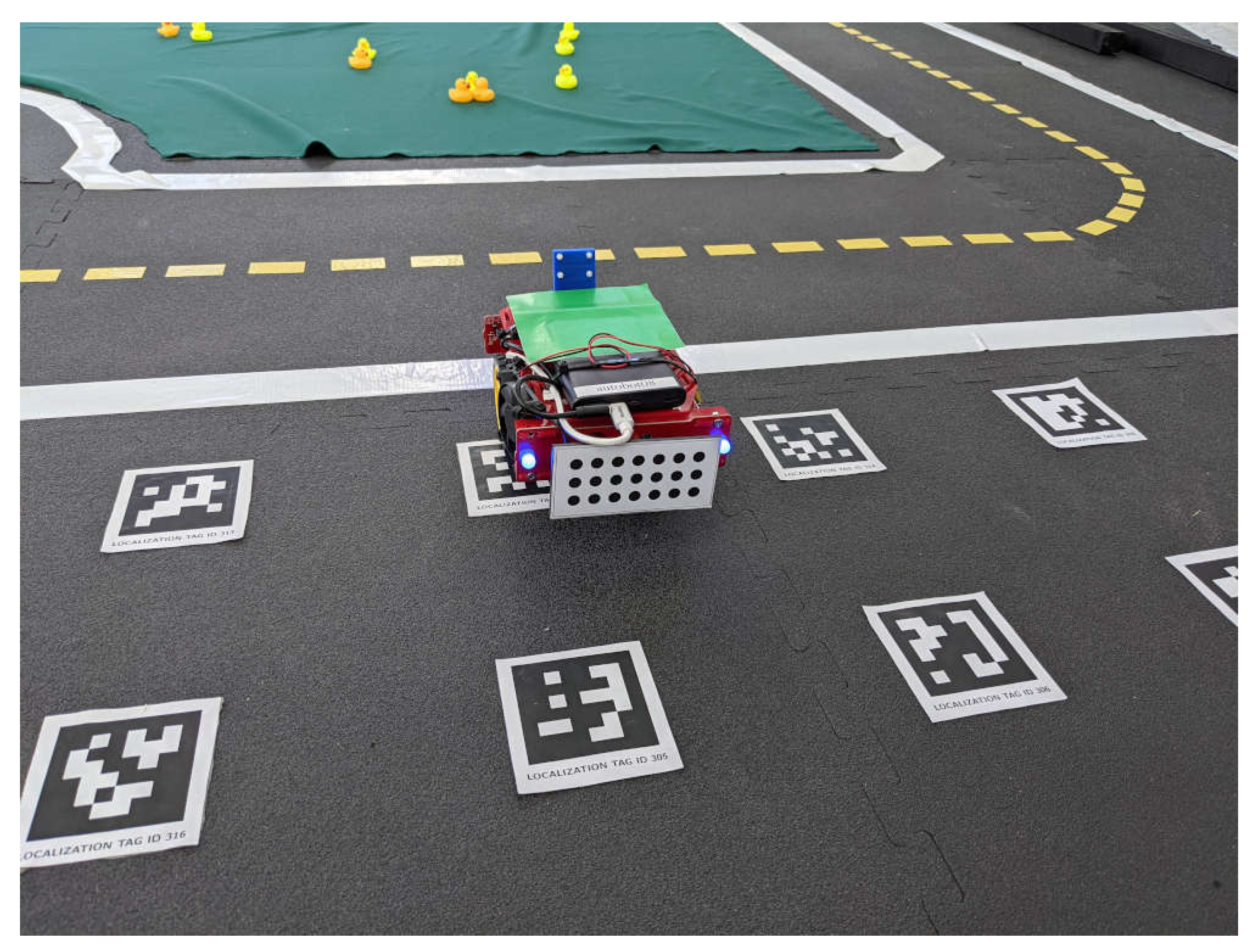
In order for the robot to take the desired position, it begins to turn in the same manner as during the data collection from the camera for calibration. The rotation direction does not matter, since in the worst case, the robot will make no more than one revolution. The rotation continues step by step until at first the robot finds at least one marker in the frame, and then until the angle of the marker rotation about its axis becomes minimal in absolute value. Since the markers were previously oriented towards the chessboards, the robot, while rotating, becomes coaxial with the marker line when the markers’ orientation around the Z axis is zero. Further, when moving the robot back and forth, it is expected to move mainly along this axis and a very wide area is not required. The location of the field with markers is shown on the left side of Figure 1.

3.4. Wheel Calibration

The main idea is to calculate the calibration coefficient of the wheels based on a series of experimental robot drives. Consider the calculations required for one experiment.

The equation of the robot’s motion can be represented as follows

$$\begin{array}{c}\hfill \left\{\begin{array}{c}{x}^{\prime }\left(t\right)=R\frac{{\omega }_1\left(t\right)+{\omega }_2\left(t\right)}{2}cos\left(\theta \left(t\right)\right)\\ y^{\prime }\left(t\right)=R\frac{{\omega }_1\left(t\right)+{\omega }_2\left(t\right)}{2}sin\left(\theta \left(t\right)\right)\\ {\theta }^{\prime }\left(t\right)=R\frac{{\omega }_1\left(t\right)-{\omega }_2\left(t\right)}{L}\end{array}\right.\end{array}$$

(1)

where

• $\theta$—robot angle,
• ${\omega }_1{\omega }_2$—angle velocities of left and right wheels;
• R—wheels radius that should be determined for a particular robot;
• L—distance between wheels that should be determined for a particular robot.

Moreover, if the movement is performed with constant angular velocities, then the differential equation turns into the usual

$$\begin{array}{c}\hfill \left\{\begin{array}{c}x=tR\frac{{\omega }_1+{\omega }_2}{2}cos\left(\theta \right)\\ y=R\frac{{\omega }_1+{\omega }_2}{2}sin\left(\theta \right)\\ \theta =tR\frac{{\omega }_1-{\omega }_2}{L}\end{array}\right.\end{array}$$

(2)

where t—movement time.

It can be seen that the orientation angle of the robot (camera) is independent of the coordinates, while the coordinates depend on the angle. Therefore, it is possible to obtain a calibration coefficient even without information about the real speed of the robot in space.

If the robot actually travels in a straight line in the world from one marker to the second, its orientation angle relative to the first and second markers should remain unchanged. This statement is based on the requirement that the markers are all oriented in the same way. However, sometimes it is possible that the robot does not move straight, even if it invokes the command of moving straight. This behavior may be caused by a slight difference in wheels radius, a slight difference oin wheel engines output torque, wheel wear, etc. To avoid this, the movement model is required to be updated.

The angle of the marker’s rotation over time can be expressed as $\Delta \theta$. Since the robot thinks that it moves with equal angular velocities of the wheels, and thinks that its angle deviation is 0, it must be pointed out that one of the wheels should be accelerated by a factor of k so that the robot rotates on $\Delta \theta$ in $\Delta t$ time. In this case, since the formula is constructed relative to the internal representations of the camera, the orientation angle of marker 2 in space should be taken. Namely, $(-\Delta \theta )$

$$-\Delta \theta =\Delta tR\frac{{\omega }_1-k{\omega }_2}{L}$$

(3)

From Equation (3), coefficient k can be expressed

$$k=\frac{{\omega }_1+\frac{\Delta \theta L}{\Delta tR}}{{\omega }_2}$$

• ${\omega }_1{\omega }_2$—angle velocities of left and right wheels;
• R—wheel radius;
• L—distance between the wheels;
• $\Delta t$—time for which the robot moved from one marker to another.

Based on this, an automatic wheel calibration algorithm is built. Let us consider the first iteration of the experiment—one robot passage—as well.

• The robot receives the orientation of the marker closest to it and remembers it.
• Next, the robot moves forward with thespeeds of the left and right wheels equal to ${\omega }_1{\omega }_2$ for some fixed time t. The speeds are calculated taking into account the calibration coefficient k, which for the first iteration is chosen to equal 1—that is, it is assumed that the real wheel speeds are equal.
• The robot obtains the orientation of the marker closest to it again and calculates the difference in angles between them.
• The coefficient $k_i$ for this step is calculated.
• The robot moves back for the same time t.

In order to reduce the influence of the error in calculating $k_i$, coefficient k is refined only by the value of $(k_i-1)/2$ after each iteration. It is important to complete this step after the robot moves back, because it reduces the chance of the robot moving outside the area width. Since the coefficient k determines the relationship between the speeds of the left and right wheels, it is always positive. If the left wheel rotates slower than the right wheel, then it will be greater than 1.0, and otherwise less than 1.0. If k is increased by $(k_i-1)/2$, then for $k_i>1$, k increases, and for $k_i<1$, k decreases. If, after the next step, the modulus of the difference between $(k_i-1)/2$ and 1.0 becomes less than the pre-selected E, then at this iteration $(k_i-1)/2$ is not taken into account. If after three successive iterations $k_i$ is not taken into account, the wheel calibration is considered to be completed.

3.5. Implementation

The camera and wheel calibration mechanism is implemented as separate ROS nodes. An existing Duckietown stack already has a software for the camera and wheel communication and for marker detection as well. Actually, the Duckietown uses Apriltags markers, and the wheel calibration node can simply subscribe to the topic with all visible markers positions.

Thus, two nodes were implemented. One is responsible for calibrating the camera, the second is for calibrating the wheels. The node responsible for calibrating the camera subscribes to the topic with camera images and, according to the algorithm described above, sends commands to the wheels to rotate the robot. Upon completion of the image collection, the standard camera calibration algorithm for OpenCV is launched. After its completion, the control is transferred to the wheel calibration node. The node in turn subscribes to the topic with the positions and orientation data of the markers found in the frame and to the topic with commands for the wheels as well. The launch of the stack for working with markers is added to the launch file with the wheel calibration node.

4. Accuracy Evaluation

4.1. Evaluated Parameters

In order to be able to compare different approaches to calibration and evaluate the quality of the suggested solution, it is necessary to set the criteria for comparing two calibration results and a criterion that allows us to evaluate the accuracy of calibration. These should be, as far as possible, objective criteria that can be measured.

For the evaluation of the camera calibration quality, it is a reprojection error. In fact, this error is proportional to the difference in the distance between the real physical point and the corresponding measured one. In other words, it describes how close to the real environment the object’s coordinates can be calculated and thus how accurately this environment can be recreated.

This value, in itself, has no dimension, and the closer this value is to zero, the better the calibration. Thus, by comparing the error value obtained as a result of the suggested algorithm and the classical manual approach, one solution evaluation can be compared to another.

To calibrate the wheels, the evaluation quality criterion needs to be determined. Unlike the camera, the result of the wheel calibration is not a matrix, but just one number—a coefficient. In fact, it determines how many times one robot’s wheel should rotate faster than another, so that when the command “move straight” is received, the robot really moves straight. However, unlike the camera, it is not so easy to determine the deviation of the obtained coefficient from the true one. The fact is that this coefficient is generally unique for each robot.

Thus, the only way to assess the quality of the wheel calibration is to compare the calibration coefficient with a known correct one. The so-called “correct” coefficient is determined by the method of manual value selection and is also not absolutely accurate. The calibration may also be affected by a coating and even a surface tilt. It is not always possible to reproduce exactly the same conditions with automatic and manual calibrations. Therefore, it is simply incorrect to evaluate how much the resulting coefficient differs numerically from the reference. A better approach is to evaluate and compare the robot’s behavior using different calibration factors.

To evaluate the robot’s behavior using this coefficient, and since the primary behavior is movement in a straight line, the comparative test should determine the quality of the robot’s movement in a straight line. Two approaches can be used for this: distance approach—when the quality can be evaluated as the robot’s deviation from the straight line, along which it begins to move when the robot passes a certain fixed distance, and a time approach—when the quality can be evaluated as the robot’s deviation from the straight line, along which it begins to move when the robot passes a certain fixed time. To evaluate the suggested solution, the distance approach was used, since it makes it possible not to depend on the speed of robot’s movement. A distance of 2 m was chosen according to the calibration validating algorithm in the Duckietown project [11].

4.2. Evaluation Methods

To compare camera calibration errors, the knowledge of how to calculate these errors is needed. Since the calibration mechanism is used by the OpenCV library, the error is also calculated by the method offered by this library.

The reprojection error when calibrating the camera is calculated as follows. The absolute deviation between the transformation outcome and the corner finding algorithm is calculated. Next, the average of these values for each image is calculated and, thereby, the total average error is calculated. Thus, each calibration will result not only in a calibration matrix, but also in a reprojection error.

To compare the suggested approach with the classical manual calibration, a series of camera calibrations was performed using the manual approach and the suggested one. After that, the mean values of errors obtained for both approaches were calculated. Thus, it enables the evaluation of the suggested solution against the currently used manual approach, given the order of the error obtained [12].

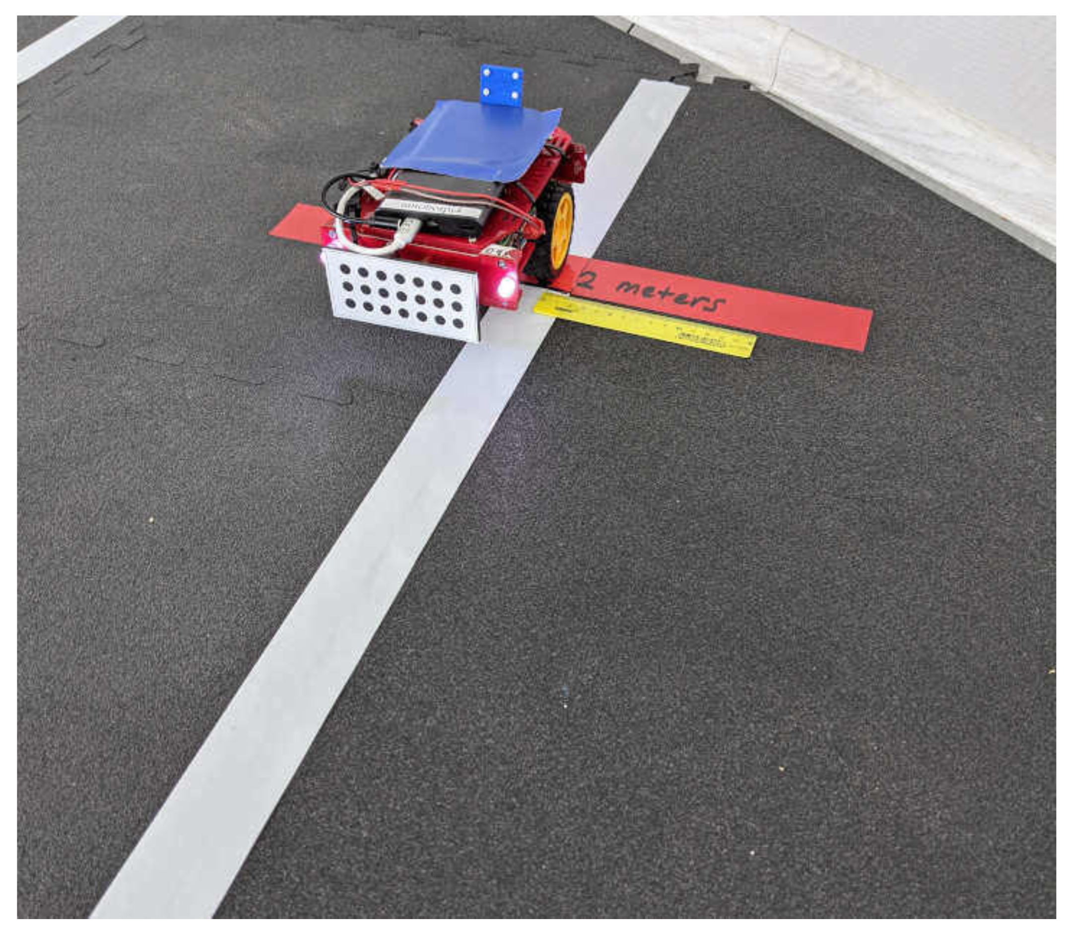
As noted earlier, with respect to calibration factors, the approach used to calibrate the camera is not applicable. Therefore, the influence of the coefficient on the robot’s trajectory curvature is estimated. To do this, the robot was located at a certain fixed distance from a straight line, along which it was oriented and then moved in manual mode strictly directly to a distance of two meters from the start point along the axis, relative to which it was oriented. Then, the robot stopped and the distance between the initial distance to the line and the final one was calculated. This difference was chosen as a calibration error. Figure 3 represents the end of the test line. The robot was originally set up so that the right edge of the right wheel was aligned with the right side of the line. The distance the robot traveled between the right side of the wheel and the edge of the line was calculated. Since the rubber protrusion of the wheel and the measurement method may not be entirely ideal, the value was rounded to the nearest hundredth of a meter.

As a reference value of the calibration coefficient, the coefficient hand-picked in the same place, but further tested in a different place, was used. This was carried out in order to exclude the value setting specifically for a certain area of coverage [11].

It is important to note that, when fully in the automatic mode, the quality of the wheel calibration is affected by the camera calibration, since the process of calibrating the wheels uses a marker recognition mechanism and therefore the calibration matrix. In order to determine the effect of camera calibration on the wheel calibration accuracy, two series of wheel calibration experiments were conducted. In one case, the same camera calibration matrix obtained in a manual mode was used, and in the other, a new camera calibration matrix obtained in an automatic mode each time was used. This made it possible to determine the relationship between the camera calibration quality and the accuracy of the wheel calibration based on it.

4.3. Calibration Results Analysis

Ten camera calibration tests were performed, manually and automatically, using the suggested algorithm. Each test was characterized by a reprojection error, and the results of comparing the manual and automatic calibration modes are presented in Figure 4a.

To calibrate the wheels, two sets of experiments were performed. The first one-used the calibration matrix that was initially the best (with the least reprojection error) and then the automatic calibration at each stage. As a reference calibration, the same value of the calibration coefficient was used, which made it possible to achieve a minimum deviation from a straight line. The deviation value is measured in meters, and the positive direction of the measurement is directed to the right side along the movement of the robot. The deviation of the first test is presented in Figure 4b, and the results of the second test can be found in Figure 4c.

The tests found that the suggested solution, on average, shows that the results are not much worse, than the classical manual solution when calibrating the camera, as well as when calibrating the wheels with a well known calibrated camera. However, when calibrating both the wheels and the camera, the wheel calibration can be significantly affected by the camera calibration effect. As a result of testing, a clear relationship was found between the reprojection error and the straight line deviation.

5. Method Modifications

5.1. Moving the Robot Out of the Calibration Area

After the integration of this approach, it became necessary to automate the last step-moving the robot to the field. Due to the fact that after the calibration step completion the robot becomes fully prepared for launching autonomous driving algorithms on it, the automation of this step further reduces the time spent by the operator when calibrating the robot, since instead of moving the robot to the field manually, he can place the next robot at the starting position. This will shorten the initialization time for a group of new robots. The current software stack of robots in use assumes the movement in a road lane with a white line along the right edge of the lane, with a yellow dashed line marking separating the lanes of different directions. When using robots from other projects, the environment it supports may be different, and the main task is to move the robot from the calibration area to the area marked out in a way suitable for the robot. In our case, the calibration field was located at the side of the road lane so that the floor markers used to calibrate the wheels are oriented perpendicular to the road lane. In other words, the floor markers in this case will be oriented in relation to the direction of the robot’s movement towards the exit from the calibration zone, which means the robot’s movement towards its standard working environment. The example is shown in Figure 5. Despite the fact that by the beginning of the wheel calibration the robot was already oriented coaxially with the markers, the robot could turn during the movement, and this condition became incorrect. This is manifested particularly strongly if the robot had a large error initially and its first movements were in a sufficiently large arc. Thus, the first stage of the robot automatic removal from the calibration zone is to return its orientation back to the same state, as it was at the moment when the wheel calibration started. This was carried out using exactly the same approach that was described earlier—depending on the orientation of the floor marker closest to the robot, the robot rotates step by step about its axis clockwise or counterclockwise until the value of the robot’s orientation angle is modulo less than some preselected value. Small deviations from the ideal orientation are not critical, since the width of the field, as described earlier, is sufficient for the robot to move not only in an ideal straight line. At this point, the robot is still on the wheel calibration field, but in this case, it is oriented towards the lane. Thus, the last step is to move the robot outside the border of the field with markers. To do this, it is enough to give the robot a command to move directly until it stops observing the markers, when the last marker is hidden from the camera view. This means that the robot has left the calibration zone, which in turn means that the robot is in the lane. This is the final stage of calibration and the robot can be put into the automatic mode. While in an automatic mode, the robot is able to continue moving in the lane and is available for control. The fact that the robot will be located in the lane at right angles to the direction of travel by the time it leaves the calibration zone is not a problem—the robot’s control algorithms, after starting their work, will determine the robot’s position in the lane, and the robot will continue moving in a standard mode. Thus, the automatic calibration algorithm is supplemented from the end with the following points:

• Orient the robot coaxially with the orientation of the floor markers;
• Move straight as long as there is at least one marker in the frame;
• Stop;
• Transfer the robot control to standard robot control algorithms.

5.2. Calibration Refinement during the Robot’s Operation

During the robot’s operation, the calibration may become irrelevant. The camera calibration can only be affected by a change in camera characteristics (camera replacement) or a change in focal length (which is fixed for these robots), so recalibration is most often required only when changing the camera, which does not happen often. The situation with recalibration of motors is somewhat different. It can be influenced by various factors: a change in the wheel diameter due to wear of the wheel coating, a slight change in the characteristics of motors due to the wear of the gearbox plastic, and a change in the robot’s weight distribution, e.g., laying the cables on the other side of the case after charging the robot, and so a slight calibration mismatch can occur. However, all these factors have a rather small impact, and the robot will still have a satisfactory calibration. There is no need to re-perform the calibration process, just a little refinement of the current one seems to be enough. It was decided to support this functionality. To do this, a section of the road along which the robots will be guaranteed to pass regularly, was selected. Depending on the algorithms of the robot and the configuration of the city, these can be different sections; in this case the section along which the robot leaves the recharging zone was chosen. Further, markers were placed in this lane according to the rules described earlier: the distance between the markers is 15 cm; the size of the marker is 6.5 cm, as presented in Figure 6. The markers are located in the center of the lane. The distance between the markers may be not completely accurate, but they should be oriented in the same direction and co-directed with the movement in the lane on which they are placed. An important condition is that the markers must be placed on a straight road section and have at least one field tile with a straight road section at the beginning and at the end of the section, the number of markers is known as well. The first marker in the direction of travel must have a predefined ID. It can be anything, the only limitation is that it must be unique for a current robot environment. Further, the following changes were made to the algorithm for the standard control of the robot: when the robot recognizes the first marker with a predetermined ID while driving right in the lane, it corrects its orientation relative to this marker and continues to move strictly straight ahead. Further, the algorithm is similar to the one described earlier—the robot recognizing the next marker can refine its wheel calibration coefficient, apply it, and change the orientation coaxially with the next marker. The number of iterations depends on the number of markers located on the calibration road segment. This approach serves to perform calibration without affecting the main task of the robot on a given segment—moving in the lane. This approach can be followed an arbitrary number of times, and since the algorithm applies new values of the calibration coefficient only when the new value is constant and significantly different from the current one, it ensures that a random error will not negatively affect the currently used coefficient.

6. Future Work

The findings of the experiments resulted in determining the relationship between the quality of camera focusing and the calibration accuracy of both the camera and the wheels. Structurally, the focal length is changed using an adjusting ring on the camera lens, which is fixed with a screw. Cameras may initially come with several different focal length settings, and some may be better suited. It was determined that the best camera calibration result is achieved when the chessboards are in maximum focus during the camera calibration. Due to the fact that the process of changing the focal length is purely mechanical, it will not be possible to fully automate it; however, the operator can be saved from the need to look at the image when adjusting the focus. It is suggested to use the image sharpness metrics and add the camera sharpness setting to the zero step performed before calibration. For this, the operator will be provided with an interface displaying the current value of the sharpness metric and its maximum, which will be reached when passing through the sharpness point [13].

7. Conclusions

As a result, a solution was developed that allows a fully automatic calibration of the camera and the robot’s wheels in the Duckietown project. The main feature is the autonomy of the process, which allows one person to run the calibration of an arbitrary number of robots in parallel and not be blocked during their calibration. In addition, the robot is able to improve its calibration as it operates in default mode. The limitation is the number of physically labeled sites.

Comparing the developed solution with the initial one resulted in finding a slight deterioration in accuracy, which is primarily associated with the accuracy of the camera calibration; however, the result obtained is sufficient for the robot’s initial calibration and is comparable to manual calibration. The planned improvements aimed at increasing the camera calibration accuracy include the use of a larger number of chessboards located at different angles and implementation of sem-automatic camera focusing. Increasing the camera calibration accuracy will automatically increase the wheel calibration accuracy.