Abstract
Aerostatic bearings are attractive, with minimal friction losses, high durability, and environmental friendliness. However, such designs have a number of disadvantages, including low load-bearing capacity and high compliance due to high air compressibility and limited injection pressure. The article proposes a double-row aerostatic journal bearing with an external combined throttling system and longitudinal microgrooves in the inter-row zone. It is hypothesized that the use of microgrooves will reduce the circumferential flows of compressed air, as a result of which the compliance should decrease and the bearing capacity should increase. To test the hypothesis, we carried out the mathematical modeling, calculations, and theoretical study of stationary operation modes of the bearing for small shaft eccentricities in the vicinity of the central equilibrium position of the shaft and bearing capacity for arbitrary eccentricities. Formulas were obtained for the numerical evaluation of compliance for bearings with a smooth bushing surface and with longitudinal microgrooves. Iterative finite-difference methods for evaluating the fields of the squared pressure are proposed, on the basis of which the load capacity of the bearings is calculated. Experimental verification of the bearing’s theoretical characteristics was carried out, which showed satisfactory agreement between the compared data. The study of the compliance and load capacity of a microgroove bearing yielded impressive results. We show that the positive effect from the application of the improvement begins to manifest itself already at four microgrooves; the effect becomes significant at six microgrooves, and at twelve or more microgrooves, the circumferential flows in the bearing gap practically disappear; therefore, the bearing characteristics can be calculated on the basis of one-dimensional models of air lubrication longitudinal flow. Calculations have shown that for a length of L = 1, the maximum load capacity of a bearing with microgrooves is 1.5 times higher than that of a conventional bearing; for L ≥ 1.5, the bearing capacity increases twice or more. The result obtained allows us to recommend the proposed improvement for practical use in order to increase the load capacity of aerostatic journal bearings significantly.
1. Introduction
Recently, there has been an increased interest in the use of aerostatic bearings in machines, particularly in machine tools and instruments. A large number of theoretical and experimental works have been published on various aspects of gas lubrication [1,2,3,4,5,6,7,8]. The greatest demand for aerostatic bearings is observed in machine-tool construction when using aerostatic bearings in the spindle units of metalworking machines [9,10,11,12].
Aerostatic bearings are attractive because of their main advantages, namely, low air viscosity, minimal friction losses, and, as a consequence, high durability and environmental friendliness [13,14,15,16].
At the same time, aerostatic bearings have a number of disadvantages, the most predominant of which are low load-bearing capacity, high compliance (low stiffness), and an increased tendency for instability. The first two drawbacks are explained by the limited injection pressure, and the last drawback is determined by the high compressibility of air, even in microvolumes [17,18]. To reduce compliance, aerostatic bearings are used with active compensation of airflow and with displacement compensators of the movable element (shaft) [19,20,21,22,23,24]. In such bearings, the problem of high compliance is solved because these types of bearings allow a decrease in compliance to zero and even negative values (in the latter case, the shaft relative to the housing is displaced in the direction opposite to the current load), which allows the structures to be used not only as supports but also as active deformation compensators of the technological system of machine tools in order to reduce the time spent and increase metalworking accuracy. A constructive innovation—the system of external combined throttling (SECT) [18]—provides a significant decrease in compliance and guarantees stability. The use of SECT can significantly increase the performance speed of bearings and improve their dynamic quality, significantly reducing the oscillation of transient processes caused by external forces, which also affects the accuracy of metalworking.
Progress towards improving compliance and stability characteristics has not, however, touched on one of the main performance characteristics of aerostatic bearings, namely, their bearing capacity. The low load capacity is not only impacted by the limited injection pressure, as there is another factor that only applies to radial aerostatic bearings. This factor relates to the presence of circumferential compressed air crossflows in the bearing gap of structures. Moreover, the longer the bearing, the greater these flows and, consequently, the lower the bearing capacity. In this paper, a method for increasing the bearing capacity by partially or almost completely suppressing the negative effect of circumferential gas lubricant crossflows in the bearing lubrication gap is considered.
However, we will first consider the characteristics of a conventional SECT aerostatic bearing since the improvements in the suppression of circumferential flows will be applied to these types of structures.
2. Characteristics of a Conventional Aerostatic Bearing
Figure 1 shows the design diagram of the structure.
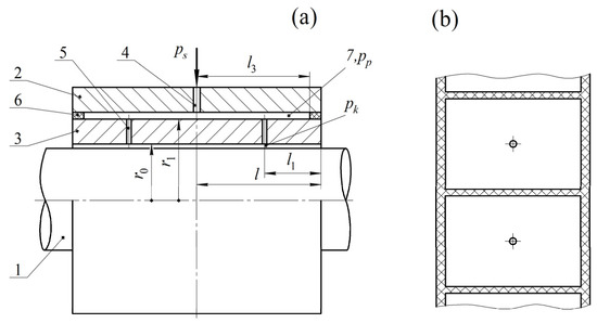
Figure 1.
Design diagram of an aerostatic journal bearing with SECT: (a) longitudinal section, (b) unfolded drawing.
An aerostatic journal bearing (Figure 1a) consists of a shaft 1 (Figure 1), a body 2, and a stationary inner sleeve 3 resting on a rigid annular suspension 6. In the body 3, throttling diaphragms 4 are made, and, in the movable sleeve 3, there are damping annular diaphragms 5, where resistance in a stable bearing should be at approximately an order of magnitude lower than the resistance of the feeders 4. This ensures maximum stability and optimal dynamic quality [18]. The surfaces of the body, bushing, and suspension form inter-throttle chambers 7, where volume plays an essential role in ensuring the optimal dynamic quality of the structure. In order to reduce the negative effect of the circumferential crossflow of air in the inter-throttle cavities on the load characteristics of the bearing, they are separated from each other by a sufficient number of longitudinal baffles, as shown in Figure 1b.
Compressed air under injection pressure ps = const (pumping source is not shown in Figure 1), overcoming the resistance of throttling feeders 4, enters the inter-throttling cavities 7 under pressure pp < ps. Further, through damping annular diaphragms 5, air enters the bearing gap under pressure pk < pp and then flows out into the environment with pressure pa.
Let us consider two mathematical models of the bearing’s stationary state—a small movement of the shaft 1 in the vicinity of its central equilibrium position and an arbitrary position at any shaft eccentricity. We will investigate the characteristics under the assumption that the axes of the bushing and bearing are parallel.
3. General Mathematical Model of the Static State of a Conventional Bearing
We will consider, in a stationary mode, small radial displacements of the shaft 1 caused by small effects from the external load f.
Let us assume that the number of annular diaphragms in each row is large enough, which makes it possible to calculate the characteristics of the bearing using the method of continuous pressurization lines, which allows the replacement of discrete pressurization holes in each row with an equivalent continuous feeder with equal pressure at its outlet while maintaining the nature of the lubricant outflow from the diaphragms [25]. Studies show that such a model is trustworthy if the number of feeders nk > 15 in each row [25]. In these cases, the error in calculating the performance of bearings with discrete feeders does not exceed 1%.
The study of the static characteristics of the bearing was carried out in a dimensionless form. The following are taken as scales of values: shaft radius r0—for lengths, radii and longitudinal coordinate z; the thickness h0 of the lubricating gap with the coaxial arrangement of the shaft and sleeve—for the current thickness h of the bearing gap and eccentricity e; the ambient pressure pa—for pressures; 2πr02pa—for forces; —for mass airflow rates, where μ is the coefficient of dynamic air viscosity, R is the gas constant, T is the absolute air temperature, and nd is the number of diaphragms in one row.
3.1. Boundary Value Problems for a Dimensionless Function of Pressure in the Bearing Gap
When the axes of the shaft 1 and sleeve 3 are parallel, the pressure function P(Z,φ) in the bearing gap satisfies the stationary Reynolds equation [26]
where Z, φ are longitudinal and circumferential coordinates.
is a function of the thickness of the bearing gap; ε is an eccentricity.
To formulate boundary conditions for Equation (1), we introduced local coordinate systems. We will consider the symmetrical right half of the bearing. In the inter-row zone 0 ≤ Z ≤ L2, in the end zone 0 ≤ Z ≤ L1, and for both of these zones 0 ≤ φ ≤ 2π, where L2 = L − L1 is half the length of the inter-row zone, L1 is the length of the end zones, and L is half the bearing length.
Let us take Ψ = P2. Then, the corresponding boundary value problem for Equation (1) takes the form
where is the squared function of the pressure on the boost line at the air outlet from the damping annular diaphragms.
The response to small loads F will be small changes in the bearing gap, eccentricity Δε, and the square of the pressures at the feeders’ outlet
where are the values of the function Ψ at the exit from the annular and simple diaphragms with the coaxial arrangement of the shaft and sleeve, are small deviations.
By analogy, let us take
Substituting (6) into (1) and performing the separation of functions, taking into account (4), we obtain the boundary value problem for the function Ψ0(Z)
and the boundary value problem for the function of small deviations ΔΨ(Z)
The solution to Problem (7) is the function
The solution to Problem (8) is the function
The dimensional bearing capacity of the bearing is calculated by the following formula [26]:
After reducing (11) to a dimensionless form, we obtain
In Formula (12), we express Ψ in terms of P. Since
then
Substituting (13) into (12), we obtain
Replacing Ψ in (1) by P, we write (10) in the form
where, taking into account (9)
Substituting (15) and (16) in (14), we obtain the formula for determining the small deviation of the bearing capacity
where
At the outlet of the pressurization line and the inlet into the bearing gap, the dimensionless gas flow rate Qh is distributed in two directions: Qh2 into the inter-row zone and Qh1 into the end zone [26]
where
Taking into account (4) and (13) and performing linearization (19), we obtain
and
Having performed the differentiation in (15) and (16), we describe the formula for the flow rate in the end zone with the central position of the shaft as
and the formula for the small deviation of the flow rate in this part as
where
Similarly, for the inter-row zone, we obtain
where
Substituting (23)–(26) into (18), we find the final formulas for the separated components of the air flow rates in the bearing gap
where
To determine the mass flow rate of air through the diaphragms, we used the formula obtained by integrating the boundary value problem for the nonlinear Bernoulli equation [26]
where
and where p1, p2 are the pressures at the inlet and outlet of the diaphragms; p1 ≥ p2, s is the effective part of the air outflow from the diaphragms ( for annular diaphragms, for simple diaphragms); and is the critical pressure ratio at the adiabatic exponent for air γ = 1.4 [26].
After reduction to a dimensionless form, we obtain the formula for the flow rate through the annular diaphragms
and the formula for the flow-through simple diaphragms
where
3.2. System of Equations for the Balance of Forces and Air Flow Rate in the SECT
The dimensionless system of equations describing the static equilibrium of the bearing includes one equation for forces and two equations for the balance of air flow rates in the SECT
It is convenient to calculate the constant static pressure Pk0 at the outlet of the damping feeders and the corresponding pressure Pp0 in the inter-throttling chambers using the normalized coefficients [18,21,24]
By setting the injection pressure Ps, χ and ς, we can find the dimensionless pressures of the unloaded bearing
With the help of (27), it is now possible to calculate the flow rate in the bearing gap. Using (35)–(37) at ε = 0, we find the criteria for the similarity of damping annular diaphragms and throttling simple diaphragms
After linearizing (33) and (34), we find the deviations of the flow rates through the diaphragms
where
From (35), it follows that the equations of forces and flow rates for deviations can be written in the form
Substituting (17), (27), (39), and (40) into (41), we obtain a system of linear equations, which can be written in matrix form as
where are the gains of the transfer functions, which are equal to the ratio of the output deviations and the small input force deviation The quantity is the static compliance of the bearing.
Having solved the system of (42), we find the static compliance of the bearing as
The resulting formula makes it possible to evaluate the effect of circumferential flows on bearing compliance at small shaft displacements.
Figure 2 shows the dependences of the compliance Ke on the length L at various values of the relative elongation of the end length λ1 = L1/L, the injection pressure Ps = 5, and the recommended values of the SECT tuning factors χ = 0.45, ς = 0.15 [18,21].
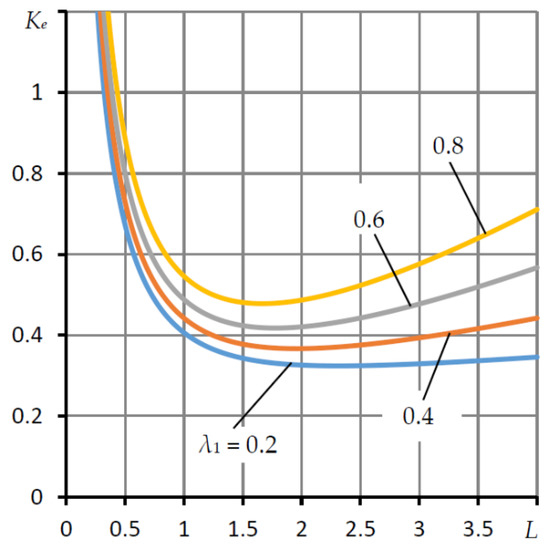
Figure 2.
Dependences of the compliance Ke of a lightly loaded bearing on the length L at different values of the relative elongation of the end zone λ1.
With an increase in L, the part of the bearing surface lubricated by air increases should contribute to a decrease in the compliance Ke. However, as the graphs show, a decrease in compliance occurs only up to a certain Lopt, which corresponds to the minimum compliance. For example, for L = 1.5 and λ1 = 0.4, the minimum compliance of Ke = 0.367 occurs at L = 1.97. With a further increase in L, the compliance begins to increase. The reason for the deterioration of compliance, in this case, is significant air crossflows. Obviously, at small eccentricities, the bearing capacity will also decrease since . In this regard, the dependences of compliance and bearing capacity for arbitrary working eccentricities (ε ≤ 0.8) are of interest.
3.3. Bearing Model with Arbitrary Eccentricities
We transform the Reynolds equation of Problem (3) and write it in the form
where
We divided the segment into an even number of m parts and segment Z ∈ [0, L] into an even number of n parts. Let us write Equation (44) in a finite-difference form [27,28]
where are the steps of integration with respect to the variables φ and Z; j = 1, 2,…, m − 1, and i = 1, 2,…, k − 1, k + 1,…, n − 1 are the numbers of the nodal points for these variables. For the injection line i = k, we composed separate equations.
We write the first boundary condition (3) in the following form [27,28]:
The second boundary condition (3) for j = 0, 2, ..., m is written in the following form:
where is the number of the point on the grid of the longitudinal axis, which corresponds to the location of the pressurization line Z = L2.
The fourth condition (3) for j = 0, 1, ..., m is
We write the last boundary conditions (3) for i = 0, 1, ..., n in the form
We represent (45) in the form
where
Applying the well-known formulas of the quadratic order of accuracy to represent the first derivative of the function at the edges of the segment [27], we write the formulas for the flow rate in the bearing gap on the pressurization line as
Corresponding to (33) and (34), the finite-difference equations of the flow rate through the orifices have the form
The final two equations in (35), as well as (52) and (53), give the system of equations
The system of Equations (46)–(50), (54), and (55) was solved by the iteration method. For this, Equation (50) at intermediate nodes is represented in the form
where j = 1, 2,…, m − 1; i = 1, 2,…, k − 1, k + 1,…, n – 1; α is the iteration number.
Similar iterative formulas on the pressurization line have the form
The pressures at the new iteration were found by solving the nonlinear equations (55). For this, they were presented in the form
For i = 0, Formula (46) is used. For this, the iterative scheme has the form
The values of Function (16) were taken as the initial value of the pressure fields at the nodal points.
Bearing load capacity
was determined by the Simpson cubature formula [29]. Calculations were performed for n = 20 and m = 20.
Figure 3 shows the graphs of the dependence of the load capacity W on the eccentricity ε at various values of the length L at λ1 = 0.5, Ps = 5, χ = 0.45, ς = 0.15.
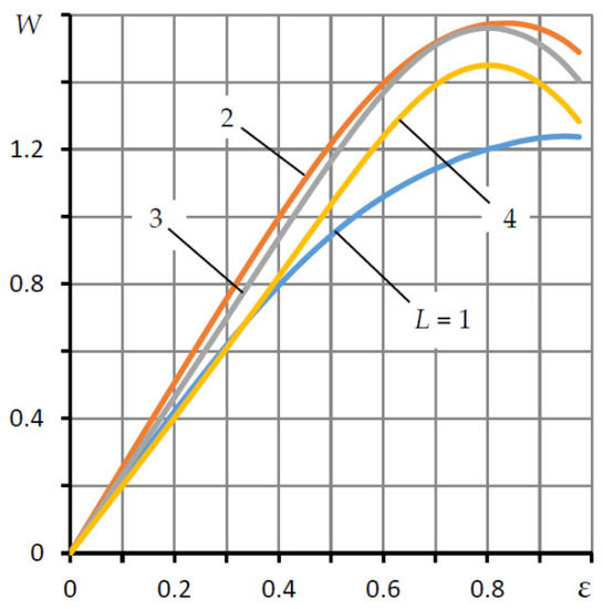
Figure 3.
Dependences of the bearing load capacity W on the eccentricity ε for different values of the length L.
It can be seen from the graphs that in the region of small and moderate eccentricities, the dependence W(ε) is close to linear and can be approximately represented by a simple formula
therefore, the bearing capacity is characterized by the same characteristic of bearing stiffness, which is the opposite of the compliance Ke. Based on this, it can be assumed that a decrease in circumferential air flows in the bearing gap will contribute not only to a decrease in compliance but also to an increase in bearing capacity, which, as mentioned above, is relevant for radial aerostatic bearings.
Further, a method for reducing circumferential flows and, therefore, reducing their effect on the compliance and bearing capacity of the bearing is considered.
4. Bearing with Longitudinal Microgrooves
The proposed improvement consists of the use of ng longitudinal microgrooves 3, which, as shown in Figure 4, are made on the bearing surface 1, at the same distance from each other.
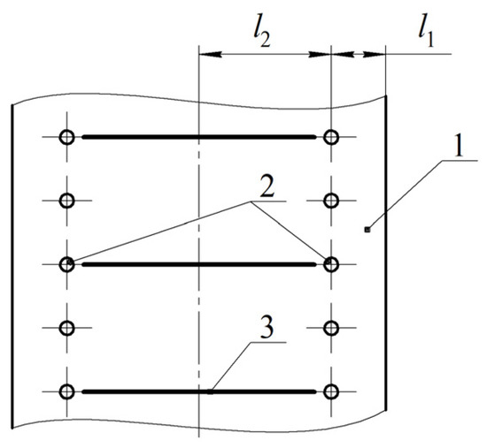
Figure 4.
Unwrapping of the supporting surface with microgrooves.
The microgrooves are located in the inter-row zone at a minimum distance from the annular diaphragms 2, in order. Firstly, this is so as not to disrupt the nature of the outflow from the diaphragms, and, secondly, it is to provide approximately equal air pressures at the outlet from the diaphragm and the entrance to the adjacent microgroove. The idea is that due to the sufficient depth and width of the microgrooves and their number, it is practically possible to eliminate circumferential air flows and, thereby, reduce the compliance of the bearing gap and increase the bearing capacity.
4.1. Modeling the Effect of the Depth and Width of the Microgroove on Circumferential Crossflows
Let us perform a one-dimensional simulation of the compressed air flow between two parallel plates with a unit gap, one of which has a depression of width LD and depth D. The injection (supply) pressure Ps is applied to the gap inlet; the pressure at the inlet to the depression is equal to P1; at the outlet the pressure is P2, and at the exit from the gap, the pressure is Pa = 1 (Figure 5).
Figure 5.
Scheme of compressed air flow in a constant gap with a depression.
The purpose of the study is to determine at what depth and width of the depression at its edges, and therefore throughout its entire length, the pressure practically does not change, which is evidence that there is nearly no resistance to airflow in the depression. This result will make it possible to determine at what depth and width of the microgroove of the bearing under study it can be assumed that the pressure upon it is constant and equal to the pressure at the outlet of the nearest diaphragm [30].
Based on (9), with a constant clearance (D = 0), the pressure can be found by the formula
If the depression is located in the middle of the gap and D > 0, then the local coordinate systems are
where
Based on (62) and (63), we find the pressures P1 and P2 from the balance equations for the flow rates at the edges of the depression
Having solved the system of the equation in (63), we obtain
where
The ratio of the pressure difference at the edges of the step, calculated by Formula (62) at D = 0 and at D ≥ 0 and calculated by formulas (64) at D = LD, is
From Formula (65), it follows that the drop in resistance to airflow through the depression is proportional to the cube of the sum of the gap value and the size of the depression. At D = 1.15, the resistance drops by an order of magnitude, and, at D = 3.64, it drops by two orders of magnitude; therefore, we can assume that at D ≥ 4, the resistance to the airflow in the depression and, consequently, in the microgrooves practically disappears. This allows us to conclude that if the depth of the microgroove is four times or more than the thickness of the lubricating gap, then the pressure in the microgroove can be approximately considered constant and equal to the air pressure at the outlet of the nearest annular diaphragm.
At the same time, it should be borne in mind that the presence of air volumes in the microgrooves can lead to a deterioration in the dynamic characteristics of the bearing. It is known that in order to maintain stability, it is necessary that additional volumes of air in contact with the bearing gap do not exceed its volume [17].
Let us make the necessary calculations. The volumes of the bearing gap and the microgrooves, respectively, are equal and where δ is the depth and width of the microgrooves. If we assume that the gap is three orders of magnitude smaller than the radius of the bearing surface , then the ratio of the volumes of the microgrooves and the bearing gap will be in excess. This ratio, as mentioned above, should not exceed kv = 1. Taking D = 4 with a margin, we obtain the maximum allowable number of microgrooves Obviously, the volume of microgrooves cannot exceed the volume of the bearing gap since the number of micro-grooves can be counted in units or tens (a more accurate estimate will be given below), but not in hundreds. Thus, the presence of microgrooves will not lead to a loss of bearing stability due to too much additional air volume in contact with the bearing gap.
4.2. Modeling Circumferential Crossflows in the Inter-Row Zone
Let us simulate circular air flows in the inter-row zone and estimate their effect on the load capacity of the air gap in this part, depending on the number of microgrooves, which are located in a circle at the same distance from each other on the lines We will assume that the number of microgrooves ng is an even number. Due to the symmetry of flows in both directions, we will consider the area as We divide the area G into sections where is the number of sections. Consider the boundary conditions for the square of the pressure in each section on the pressurization line and microgrooves
For the boundary Z = 0, due to the symmetry of the flow, we will use the second condition of the boundary value problem (3).
We divide each section into parts and perform a finite-difference replacement of the differential equation of Problem (3). In this case, we obtain an algebraic boundary value problem for the system of Equation (50) with boundary conditions (46), (49), and (66). We solve the problem using the iteration method, using Formula (56) for the interior points. For the boundary points of the region, we use Formulas (66) and (59). The load capacity of the compressed air gap in the G region was found by summing the force reactions on the Gk segments
In the absence of circumferential flows, , therefore
Figure 6 shows the dependences of the bearing capacity W of the compressed air gap in the region G on its length L for a different number of microgrooves ng at Pk0 = 3, ε = 0.75.
Figure 6.
Dependences of the bearing capacity W of the sectors on their length L for various numbers of microgrooves ng.
The graph shows that an increase in the number of grooves begins to noticeably affect the bearing capacity immediately. Already at ng = 4, in comparison with the graph for ng = 2, at which there are no barriers to crossflows, W increases by 11%. However, a significant jump in the growth of the characteristic is observed at ng = 6. For this number of microgrooves, W increases immediately by 39%. With a further increase in the number of microgrooves, W increases in a weaker manner. Thus, at ng = 8, the growth is 48%, and at ng ≥ 12, circumferential air crossflows practically cease, providing an overall efficiency of increasing the bearing capacity from the use of longitudinal microgrooves by 61%. With other parameters, the efficiency may differ from the given estimates and is in the range of 60–75%.
The data provided testifies to the high efficiency of the use of longitudinal microgrooves to increase the bearing capacity of compressed air in the row-to-row sector of the bearing surface. If we assume that the number of microgrooves ng = 12 is optimal, then the refined estimate of their volume in relation to the volume of the bearing gap will be only 3%. Such an insignificant increase in the volume of compressed gas adjacent to the bearing gap cannot contribute to the deterioration of the dynamics of the structure; therefore, the use of microgrooves to significantly improve the static characteristics of the bearing is quite justified.
4.3. Modeling Circumferential Flows in End Regions
Circumferential flows can affect the reduction in load-bearing capacity and increase compliance in the end regions. Obviously, this influence will be smaller since the width of the end regions is usually smaller and, at the exit from the bearing gap, the pressure is constant and equal to the ambient pressure. At the same time, it is of interest to study the effect of the width of the end regions and eccentricity in order to assess at what width the circumferential flows have little effect on the bearing capacity.
We divide the segment [0, L1] into n parts and the arc [0, π] into m parts. The basic finite-difference equations (56) will be slightly modified, where x = j − 1, y = j + 1. Due to the symmetry of the air pressure at φ = 0 and φ = π, we assume x = 1, if x = −1, and y = m − 1, if y = m + 1. Taking this into account, iterative Formula (56) takes the form
where j = 0, 1, ..., m; i = 1, 2,…, n − 1, α is the iteration number.
The boundary conditions for Z = L1 correspond to the conditions in (48). The boundary conditions in (66) will be used on the pressurization line Z = 0.
For comparison, let us find the bearing capacity of an ideal model in which there are no circumferential flows. In this case, the solution to the boundary value problem is the function
The bearing load capacity can be determined numerically by the formula
The results of modeling circumferential flows on the end zones are shown in Figure 7. Graphs of the dependence of the bearing capacity W on the width L1 of the end zone are plotted for various values of the eccentricity ε. Solid lines show the dependences obtained by the iterative method. The dashed lines correspond to the ideal airflow model, where there are no circumferential flows.
Figure 7.
Dependencies of the load capacity W of the end zones on their length L1 for different eccentricities ε.
It can be seen from the graphs that circumferential flows affect the decrease in the bearing capacity only at L1 > 0.4. Such a significant width is not typical for the location of the pressurization lines; therefore, at L1 ≤ 0.4, we can assume that there are no circumferential flows in the end regions.
4.4. Ideal Air Flow Pattern without Circumferential Crossflows
Studies have shown that if the number of microgrooves is ng ≥ 12 and the width of the end regions is L1 ≤ 0.4, then when calculating the compliance and bearing capacity, circular air flows in the bearing gap can be neglected. Let us consider two models of shaft motion—for small and arbitrary eccentricities.
4.4.1. Non-Crossflowing Model for Small Eccentricities
In the absence of crossflows, the differential equation of Problem (8) takes the form
Taking this and (13) into account, the solution to the problem is the function of small pressure deviation
Substituting (68) into (14), we obtain
where
The formula for the flow rate in the bearing gap near the pressurization line has the form
where corresponds to (30). Formulas (39) and (40) remain unchanged.
Substituting the obtained simplified Formulas (69) and (70) into (43), we obtain the formula for bearing compliance without circumferential air flows in the bearing gap for small deviations of functions from the central equilibrium position of the shaft.
Figure 8 shows the dependences of the compliance Ke on the length L at various values of the injection pressure Ps for λ1 = 0.2, χ = 0.45, and ς = 0.15. The solid lines show the characteristics of a conventional bearing, and the dashed lines show the bearing with longitudinal microgrooves (ng ≥ 12). It can be seen that at L > 0.5, the use of microgrooves contributes to a significant decrease in bearing compliance. Thus, at Ps = 3 and L = 1.5, the compliance decreases by 65%, and at L = 2, the compliance is halved. For L > 2, the difference will be even greater. A similar difference is observed at Ps = 5.
Figure 8.
Dependences of the compliance Ke of a lightly loaded bearing on the length L at different values of injection pressure Ps, λ1 = 0.2.
4.4.2. Non-Crossflowing Model for Arbitrary Eccentricities
In the absence of crossflows, the pressure and air flow rate in the lubricating gap, by analogy with (16) and (23), are determined by the formulas
Formulas (33) and (34) remain unchanged.
As before, we will divide the arc into m parts. Let us set ε, and for , calculate H. Next, for each j, we solve the system of the final two nonlinear equations in (35), representing the balance of flow rates in the SECT as
relative to unknown pressures.
Having evaluated the pressure vector at the outlet of the annular diaphragms , we found the integral of the bearing capacity by the Simpson quadrature formula
where sj are the coefficients of the Simpson formula [29].
Figure 9 shows the graphs of the dependences of the bearing capacity W on the eccentricity ε calculated by Formula (71) for various values of the length L for Ps = 5, λ1 = 0.2, χ = 0.45, ς = 0.15, and ng ≥ 12. The graphs are similar to Figure 2.
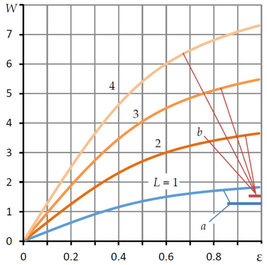
Figure 9.
Dependences of the bearing capacity W of the bearing with microgrooves on the eccentricity ε at different values of length L.
Position a in the figure indicates the maximum value of the bearing capacity W of a conventional bearing of length L = 1, and position b indicates the maximum value of W curves for L > 1 (these curves are shown in Figure 2). With L = 1, the maximum bearing capacity of a bearing with microgrooves is 1.5 times greater than that of a conventional bearing; with L = 1.5, it is 1.8 times greater; with L = 2, it is 2.3 times greater; and with L = 4, it is 4.5 times greater. The same estimates take place for small and moderate values of eccentricity.
The data obtained show that the use of longitudinal microgrooves in the inter-row zone at L ≥ 1 makes it possible to reduce the compliance by a factor of 1.5 and increase the bearing capacity. Moreover, the larger the relative length of the bearing, the better the performance. Therefore, the use of longitudinal microgrooves is an effective way to improve the force characteristics of a radial aerostatic bearing significantly.
5. Comparative Analysis of Theoretical and Experimental Data
For experimental verification of the formulas obtained, the bearing capacity of a single throttling bearing without microgrooves was found, and its compliance, stiffness, and load capacity were compared with the data of [31]. In addition, for a correct comparison, the parameter of the relative spreading of the pressurization lines λ1 = 0.5 was adopted. Comparative data are shown in Table 1.

Table 1.
Comparative bearing characteristics at relative eccentricity ε = 0.5.
As can be seen from the table, on the whole, the experimental and theoretical data are in satisfactory agreement. The theoretical bearing capacity is slightly higher than the experimental data. The reason is probably that the theoretical model is based on the assumption that discrete feeders can be replaced with a continuous pressurization line. As can be seen, this assumption gives an error of no more than 10%, which can be considered a completely satisfactory agreement between theory and experiment. This tendency is also observed when comparing the stiffness characteristics for L = 1.5. For L = 1.0, on the contrary, the theoretical stiffness was less than the experimental one.
Figure 10 shows the experimental values of W (points) obtained by Cunningham [32] for an aerostatic bearing with two sets of orifices of the “simple diaphragm” type for h0 = 33 × 10−6 mm, n = 6, d = 0.56 mm, L = 1.5, and L1 = 0.
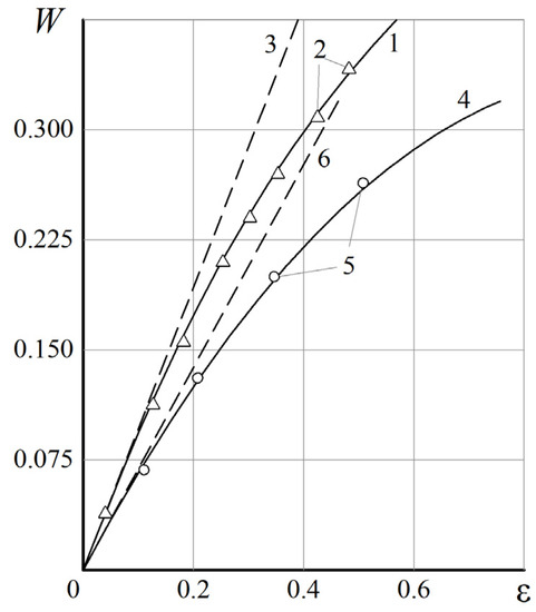
Figure 10.
Comparison of the load characteristics of a double-row bearing.
Dependencies 1 and 4 were obtained by Shatokhin [33], 2 and 5 are points of the Cunningham experiment [32], and 3 and 6 are calculated by the formula
The former corresponds to Ps = 6, the latter Ps = 2.3.
Linear dependences 3 and 6, presented in Figure 10, have a satisfactory coincidence with the compared data in the region of small eccentricities ε.
6. Conclusions
The paper considers a double-row symmetric aerostatic radial bearing with an external combined throttling system and longitudinal microgrooves in the inter-row zone. It is hypothesized that the use of microgrooves will reduce the circumferential flows of compressed air, as a result of which the compliance should decrease and the bearing capacity should increase.
To test the hypothesis, mathematical modeling, calculations, and a theoretical study of the stationary operating modes of the bearing were carried out on the assumption that when the journal moves, the axes of the shaft and sleeve remain parallel. A study of compliance for small eccentricities of the shaft in the vicinity of the central equilibrium position of the shaft and the bearing capacity for arbitrary eccentricities was carried out. Formulas were obtained for the numerical evaluation of compliance for bearings with a smooth bushing surface and with longitudinal microgrooves. Iterative finite-difference methods for determining the fields of the squared pressure were proposed, on the basis of which the load capacity of the bearings was calculated. Experimental verification of the theoretical characteristics of the bearing was carried out, which showed a satisfactory agreement of the compared data.
The study of the compliance and load capacity of a microgroove bearing yielded impressive results. It is shown that the positive effect from the application of the improvement begins to manifest itself already at four microgrooves; at six microgrooves, it becomes significant, and at twelve or more microgrooves, circumferential flows in the bearing gap practically disappear; therefore, the load characteristics can be calculated on the basis of one-dimensional models of the longitudinal flow of air lubrication. The calculations have shown that with a length of L = 1, the maximum bearing capacity of a bearing with microgrooves is 1.5 times greater than that of a conventional bearing; for L ≥ 1.5, the bearing capacity doubles or more. The result obtained allows us to recommend the proposed improvement for practical use in order to increase the load capacity of radial aerostatic bearings significantly.
It is also shown that the increase in the volume of compressed gas in the bearing gap due to the presence of microgrooves is only a few percent of a similar volume of a conventional bearing. On this basis, it was concluded that this circumstance cannot affect the deterioration of dynamic characteristics. It should be noted that bearings with combined external throttling systems have a large margin of stability, which guarantees the operability of bearings with microgrooves.
Thus, the proposed double-row aerostatic radial bearing with longitudinal microgrooves in the inter-row zone can find practical application as a better replacement for conventional aerostatic bearings in order to reduce compliance and significantly increase the bearing load capacity.
Author Contributions
Conceptualization, V.K.; formal analysis, A.K.; investigation, S.S., O.G., I.P. and Y.P.; data curation, M.B. and L.S.; writing—original draft preparation, V.K.; writing—review and editing, A.K.; project administration, A.K. and O.G. All authors have read and agreed to the published version of the manuscript.
Funding
This research received no external funding.
Institutional Review Board Statement
Not applicable.
Informed Consent Statement
Not applicable.
Data Availability Statement
The data presented in this study are available on request from the corresponding author. The data are not publicly available due to privacy.
Conflicts of Interest
The authors declare no conflict of interest.
Nomenclature
| H, h, h0 | dimensionless thickness, thickness of the gap, and its thickness for ε = 0 |
| Ke | dimensionless compliance of bearing |
| l, L | half of the length and dimensionless length of bearing |
| l1, L1 | half of the length and dimensionless length of end zones |
| l2, L2 | length and dimensionless length of the inter-row zones |
| P (Z,φ) | dimensionless dynamic pressure in the bearing gap |
| P0(Z) | dimensionless static pressure in the bearing gap for ε = 0 |
| pa | ambient pressure |
| pk | air pressure on annular diaphragms |
| pp | air pressure in inter-throttle chambers |
| ps | supply pressure |
| Qh | dimensionless flow rate through the gap |
| Qk | dimensionless flow rate through annular damping diaphragms |
| Qp | dimensionless flow rate through simple diaphragms |
| r0 | the shaft radius |
| W | dimensionless bearing capacity |
| Z | dimensionless longitudinal coordinate |
| ε | dimensionless eccentricity |
| φ | dimensionless circumferential coordinate |
| μ | coefficient of dynamic viscosity of the air |
| χ | normalized adjustment coefficient of the external throttling system |
| ς | normalized adjustment coefficient of annular damping diaphragms |
References
- Al-Bender, F. Air Bearings: Theory, Design and Applications; John Wiley & Sons: Hoboken, NJ, USA, 2021; p. 592. [Google Scholar]
- Zhang, J.; Han, D.; Song, M.; Xie, Z.; Rao, Z.; Zou, D. Theoretical and experimental investigation on the effect of supply pressure on the nonlinear behaviors of the aerostatic bearing-rotor system. Mech. Syst. Signal Process. 2021, 158. [Google Scholar] [CrossRef]
- Wang, X.; Zhou, L.; Huang, M.; Yue, X.; Xu, Q. Numerical investigation of journal misalignment on the static and dynamic characteristics of aerostatic journal bearings. Measurement 2018, 128, 314–324. [Google Scholar] [CrossRef]
- Jeng, Y.; Chang, S. Comparison between the effects of single-pad and double-pad aerostatic bearings with pocketed orifices on bearing stiffness. Tribol. Int. 2013, 66, 12–18. [Google Scholar] [CrossRef]
- Morosi, S.; Santos, I.F. Active lubrication applied to radial gas journal bearings. Part 1: Modeling. Tribol. Int. 2011, 44, 1949–1958. [Google Scholar] [CrossRef]
- Chang, S.; Chan, C.; Jeng, Y. Numerical analysis of discharge coefficients in aerostatic bearings with orifice-type restrictors. Tribol. Int. 2015, 90, 157–163. [Google Scholar] [CrossRef]
- Li, Y.; Zhou, K.; Zhang, Z. A flow-difference feedback iteration method and its application to high-speed aerostatic journal bearings. Tribol. Int. 2015, 84, 132–141. [Google Scholar] [CrossRef]
- Du, J.; Zhang, G.; Liu, T.; To, S. Improvement on load performance of externally pressurized gas journal bearings by opening pressure-equalizing grooves. Tribol. Int. 2014, 73, 156–166. [Google Scholar] [CrossRef]
- Fang, C.; Huo, D.; Huang, X. A comprehensive analysis of factors affecting the accuracy of the precision hydrostatic spindle with mid-thrust bearing layout. Int. J. Adv. Manuf. Technol. 2021. [Google Scholar] [CrossRef]
- Chen, G.; Chen, Y. Multi-Field Coupling Dynamics Modeling of Aerostatic Spindle. Micromachines 2021, 12, 251. [Google Scholar] [CrossRef]
- Chen, G.; Chen, Y.; Lu, Q.; Wu, Q.; Wang, M. Multi-Physics Fields Based Nonlinear Dynamic Behavior Analysis of Air Bearing Motorized Spindle. Micromachines 2020, 11, 723. [Google Scholar] [CrossRef] [PubMed]
- Chen, P.; Zhuang, H.; Chang, Y.; Ding, J.; Zhong, Q.; Yang, H. Modal analysis of an aerostatic spindle system for ultra-precision machine tools at different spin speeds. Adv. Mech. Eng. 2018, 10. [Google Scholar] [CrossRef] [Green Version]
- Majumdar, B. On the General Solution of Externally Pressurized Gas Journal Bearings. J. Lubr. Technol. 1972, 94, 291–296. [Google Scholar] [CrossRef]
- Mori, A.; Mori, H. An Application of Pneumatic Phase Shifting to Stabilization of Externally Pressurized Journal Gas Bearings. J. Lubr. Technol. 1973, 95, 33–41. [Google Scholar] [CrossRef]
- Viktorov, V.; Belforte, G.; Raparelli, T. Modeling and Identification of Gas Journal Bearings: Externally Pressurized Gas Bearing Results. J. Tribol. 2004, 127, 548–556. [Google Scholar] [CrossRef]
- Lai, T.-H.; Chang, T.-Y.; Yang, Y.-L.; Lin, S.-C. Parameters design of a membrane-type restrictor with single-pad hydrostatic bearing to achieve high static stiffness. Tribol. Int. 2017, 107, 206–212. [Google Scholar] [CrossRef]
- Pinegin, S.; Tabachnikov, Y.; Sipenkov, I. Static and Dynamic Characteristics of Gas-Static Supports; Nauka: Moscow, Russia, 1982; p. 265. [Google Scholar]
- Kodnyanko, V.; Shatokhin, S. Theoretical study on dynamics quality of aerostatic thrust bearing with external combined throttling. FME Trans. 2020, 48, 342–350. [Google Scholar] [CrossRef]
- Kodnyanko, V.; Pikalov, Y.; Shatokhin, S. Investigation of the characteristics of a gas-static bearing with active flow rate compensation. Bull. Mech. Eng. 1979, 4, 9–12. [Google Scholar]
- Shatokhin, S.; Kodnyanko, V. Load and flow rate characteristics of an axial pressurized gas bearing with an active compensation of gas flow. Springer Nat. Mech. Sci. 2017, 110–115. [Google Scholar]
- Shatokhin, S.; Kodnyanko, V. Radial gasostatic bearing-seal with opposite internal gas flow compensation. Sov. J. Frict. Wear 1984, 32–35. [Google Scholar]
- Kodnyanko, V. Characteristics of a gas-static thrust bearing with an active displacement controller. Mosc. J. Met. Cut. Mach. Tools 2005, 9, 32–34. [Google Scholar]
- Kodnyanko, V.; Kurzakov, A. Static characteristics of hydrostatic thrust support with a membrane displacement compensator. Russ. Bull. Mech. Eng. 2017, 8, 66–70. [Google Scholar]
- Kodnyanko, V. Characteristics of a gas-static thrust bearing with an active displacement regulator. Russ. J. STIN 2005, 9, 32–34. [Google Scholar]
- Stepanyants, L.; Zablotsky, N.; Sipenhov, I. Method of Theoretical Investigation of Externally Pressurized Gas-Lubricated Bearings. J. Lubr. Technol. 1969, 91, 166–170. [Google Scholar] [CrossRef]
- Constantinescu, V.N. Gas Lubrication; American Society of Mechanical Engineering: New York, NY, USA, 1969; p. 621. [Google Scholar]
- Demidovich, B.; Maron, I.; Shuvalova, E. Numerical Methods of Analysis. Approximation of Functions, Differential and Integral Equations, 5th ed.; Lan: Moscow, Russia, 2010; p. 400. [Google Scholar]
- Samarskiy, A.; Nikolaev, E. Methods for Solving Grid Equations; Nauka: Moscow, Russia, 1978. [Google Scholar]
- Dwight, H. Tables of Integrals and Other Mathematical Data; The Macmillan Company: New York, NY, USA, 1961. [Google Scholar]
- Balasan’yan, V.S. Flat rectangular aerostatic bearing with a microgroove. Fluid Dyn. 1973, 8, 644–647. [Google Scholar] [CrossRef]
- Jiří, Š.; Jan, K.; Pavel, S. Dynamic properties of aerostatic journal bearings. In Colloquium Dynamics of Machines; Institute of Thermomechanics: Prague, Czech Republic, 2007. [Google Scholar]
- Cunningham, R.; Fleming, D.; Anderson, W. Steady-State Experiments on Rotating Externally Pressurized Air-Lubricated Journal Bearings. J. Lubr. Technol. 1970, 92, 336–345. [Google Scholar] [CrossRef]
- Shatokhin, S. Calculation of the characteristics of radial gas suspensions. In Improving the Accuracy and Productivity of Processing on Machines; Shatokhin, S., Ed.; Krasnoyarsk Polytechnic Institute Publishing House: Krasnoyarsk, Russia, 1973; pp. 60–69. [Google Scholar]
Publisher’s Note: MDPI stays neutral with regard to jurisdictional claims in published maps and institutional affiliations. |
© 2021 by the authors. Licensee MDPI, Basel, Switzerland. This article is an open access article distributed under the terms and conditions of the Creative Commons Attribution (CC BY) license (https://creativecommons.org/licenses/by/4.0/).