Accuracy Analysis of the Measurement of Centre of Gravity and Moment of Inertia with a Swing

Abstract

Floating devices under wave and current loads are typically designed based on numerical methods followed by a validation with experimental investigations. This allows an independent check due to the comparison of two different modelling approaches based on different assumptions. At an early stage of the project, numerical simulations are based on theoretical (ideal) values of the centre of gravity (CG) and moment of inertia (MI). The building process of a scaled model results very often in a requested simplification of certain parts, which can influence the CG and also the MI of the scaled model. Knowing those discrepancies allows us to improve the comparability of both approaches but the measurement of those values is connected with either a higher uncertainty or a high level of effort. A significant improvement of such measurements can be reached by the deployment of a specific experimental set-up. This paper presents the classification of the newly designed swing with a high accuracy inertial inclinometer, which was verified by the marker-based motion capturing system. The achieved experiences are useful for the future use of the set-up as well as similar investigations. The comparison with the theoretical values for the swing as well as an example model showed very good agreements and a high accuracy of few millimetres for the CG and an error smaller 1% for MI.

1. Introduction

The exact knowledge of the ten inertia parameters, which include the location of the centre of mass and the inertia tensor, is critical for many applications including the motion of rigid bodies. Schedlinski & Link [1] provide an overview of the different available quantification of those parameters and divides them into static and dynamic methods. A measurement and calculation of the static equilibrium of forces and torques allows only the mass and centre of gravity (CG) of the investigated object to be determined. The dynamic methods are further grouped into methods with no limitation on rigid-body motion, large angular motions with small rotational velocities and small angular motions [1]. The method based on the principle of the gravitational pendulum belongs to the latter mentioned category and simplifies the problem to a physical pendulum. The necessary equations are presented in Section 2.4. The quality of the results is dependent on an accurate measurement of the distance between the centre of gravity and the pivot point. This approach is reduced to a one degree-of-freedom problem similar to a torsion pendulum method, which can be used to measure rotational inertia [2,3,4]. This approach is practical to conduct, measure and analyse the properties of rigid bodies. The other dynamic methods require force and displacement measurements and have to be calibrated carefully [5].

Large engineering objects, for example, vehicles, are typically investigated based on an approach where they are hung from four points [6,7] or placed on a frame with four load cells [8]. Similar experimental set-ups can be found in the literature, which are limited to three rods [9,10] or three load cells [11,12]. Zhan et al. [13] report solutions to measure extremely large cylindrical objects with two rail-based measurement devices each including four load cells. Suhaimi et al. [14] present an example application of the investigation of a heavy duty vehicle deploying a mobile crane to lift and hold the armoured vehicle. For vehicle applications the inertia parameters are critical for drive dynamic, stability [15,16] as well as crash studies.

The position of the centre of gravity as well as the moment of inertia are essential input for the simulation of motions and forces of floating devices. CG is especially important for ships [17,18] and floating structures [19] including falling lifeboats [20] or floating wind turbines [21]. New and refitted ships are typically investigated with an inclination test [22,23] to ensure the precise location of the CG and that the desired stability is achieved. In the case of scaled experimental devices, the distances have to be scaled based on the specific scaling similarity [24]. The outer shape as well as the correct mass (distribution) can typically be reached to a high degree of accuracy in the scaled model. Ballasting constraints and instrumentation requirements typically lead to larger relative tolerances for the exact location of the CG as well as the MI. However, even if the CG target can not be met, accurately assessing the location at model scale allows the error to be incorporated in the subsequent analysis. Typically, this involves some form of numerical modelling in which the model CG and inertia properties can be recreated and compared to the full-scale prototype.

The paper presents the experimental set-up with the new swing, which is part of the FloWave Ocean Energy Research Facility [25,26,27,28,29] at The University of Edinburgh. The measurement procedure and the relevant equations are described in Section 2. Section 3 provides the detailed results and analysis for the CG and MI for the empty swing as well as an example measurement for a simple model. The practical implementation of the system is discussed in Section 4, including lessons learned for future measurements as well as potential improvements. Section 5 summarises the findings and provides an outlook on future research questions.

2. Materials and Methods

2.1. Construction and Theoretical Values of the Swing

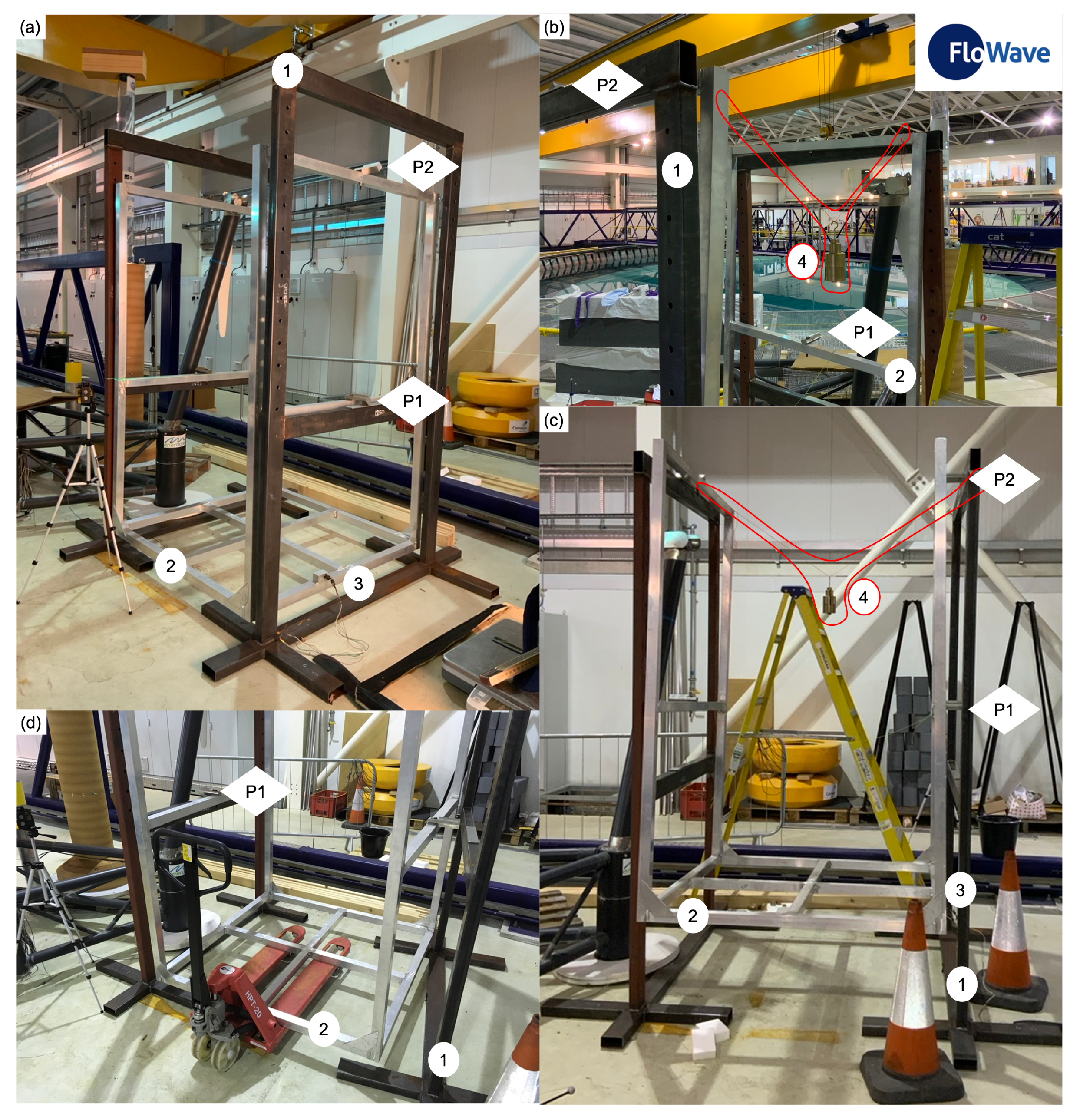
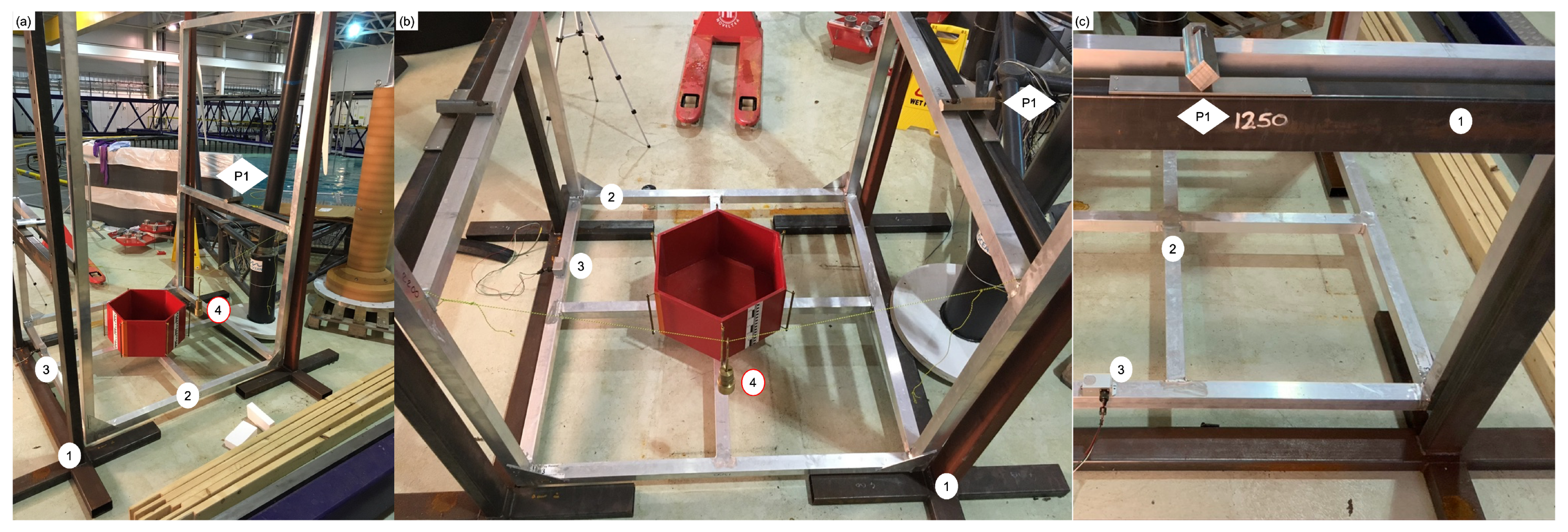
The newly constructed swing is split into two parts: (1) support structure and (2) the swing itself. Figure 1 presents an overview of the experimental set-up. The support structure is made of two identical steel frames providing a stable support due to its mass and the extended footprint. It can be moved by two persons and allows the use of two different pivot axes of the swing. This oscillating part is made of aluminium to reduce the total mass of the moving section. It has an inner spacing of 1.3 by 1.3 m and is open at the top to enable crane access. 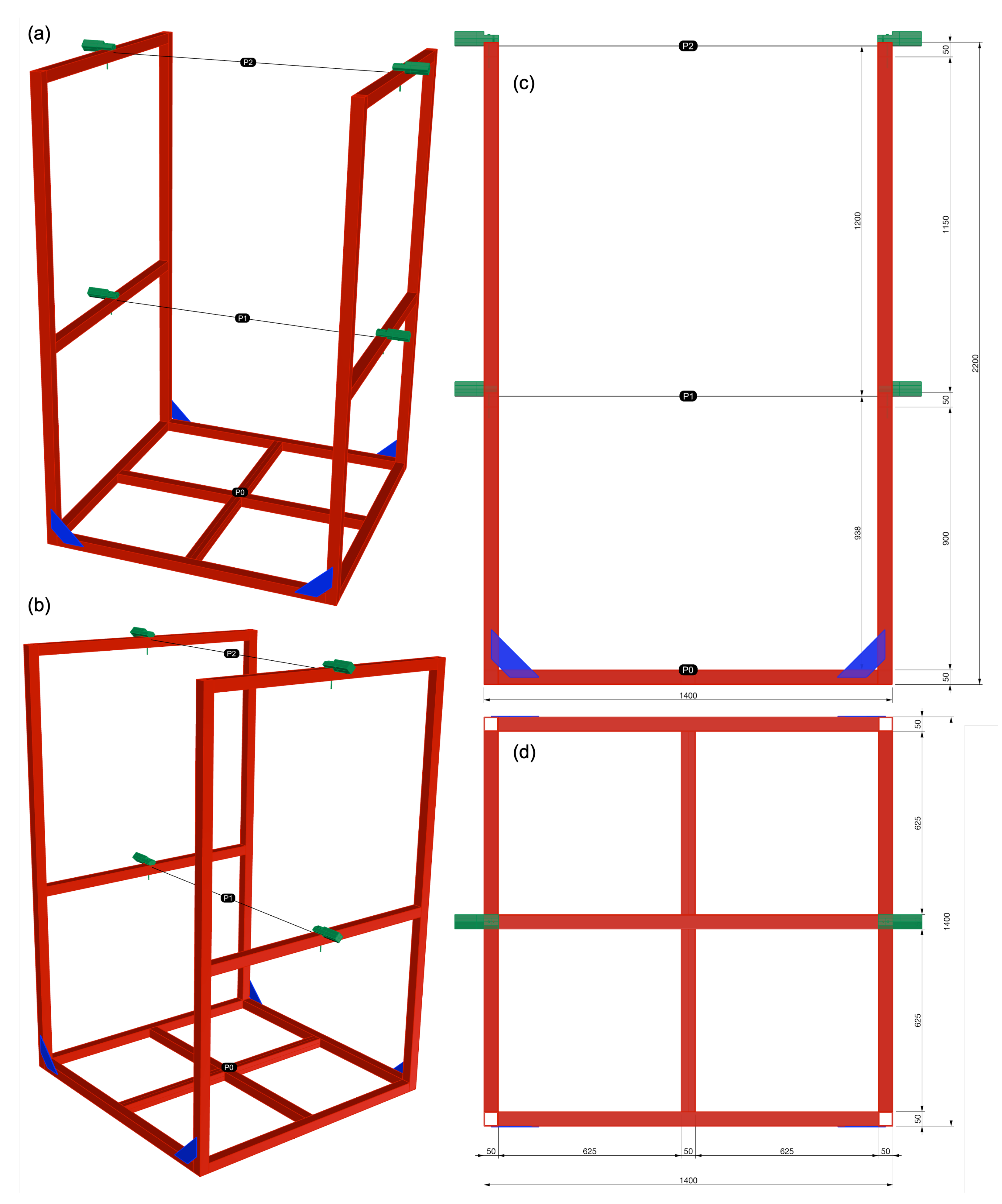The blade edges are constructed of a quadratic stainless steel profile, which is machined to ensure a sharp edge by mounting it with an angle of 45$°$ onto the aluminium profiles. Those parts are coloured green in Figure 2, which presents the dimensions of the swing.

The values presented in

Table 1. Properties of the two parts of the swing—Frame includes the red and blue elements shown in Figure 2 and the four pivot blocks are shown in green—the reference for the distance to the centre of gravity (CG) is the height P1. Moment of inertia I is based on theoretical calculations.

Name	Volume	Density	Mass	CG Part	I${}_{\mathit{P}1}$	I${}_{\mathit{P}2}$
	(m${}^3$)	(kg/m${}^3$)	(kg)	(m)	(kg/m${}^2$)	(kg/m${}^2$)
frame	0.013544	2700	36.568	0.165	35.423	102.540
4 pivot blocks	0.000681	7850	5.345	−0.624	4.007	3.698
mass difference			0.067	0.963	0.062	0.314
inclinometer			0.300	0.917	0.252	1.344

are theoretical values based on the CAD model [30] constructed with the software Rhinoceros. The only exception is the mass of the inclinometer (Section 2.2), which is measured with a typical length of cable. The sum of the theoretical masses is 41.913 kg, which is slightly lower than the measured value of 41.980 kg (measurement conducted without the approximately 0.3 kg for the inclinometer). This difference may be caused by the weld bead at the bottom of the structure, which is neglected in this theoretical approximation. Based on these values, the total centre of gravity (CG) is 72.2 mm (Table 1) under the pivot axis P1 and 1272.2 mm relative to P2 (Figure 2). A value of 64.4 mm is found based on the theoretical mass of the swing (neglecting the inclinometer). The measured mass of the swing gives a value 0.067 kg greater than the theoretical value. This calculation is based on the assumption of a point mass located a half profile under P0 and half inclinometer over P0. The comparison with the measurement of the CG is presented in Section 3.1 and Section 3.3 focuses on the evaluation of the oscillation period, which leads to the calculation of the MI.

2.2. Measurement Instrument

Two different measurement systems are deployed to observe the inclination and the oscillation of the swing: (a) inertial inclinometer and (b) the motion capturing system. The latter is included as a verification instrument and covers oscillation for which the chosen inclinometer is not fast enough. It would not be required for routine deployment of the swing. A laser level helps to reduce the effort in the installation phase especially when an additional model is loaded in the swing.

The inclination of the swing is measured with a gravity referenced inclinometer provided by Sherborne (model LOCS 3) [31]. Such an instrument is typically used in industrial applications including bore-hole mapping, pipeline levelling and observation of big structures such as dams, ships or barges as well as bridge deformation [32] and medical applications for precise alignment of imaging systems [33]. The measurement range of the inertial inclinometer covers ±3$°$ resulting in a full range output (FRO) of 6$°$. Based on the manufacturer’s information [31], the non-linearity (NL) of 0.05% of FRO and the non-repeatability (NR) 0.02% of FRO, which results in a $e_{NL}$ of $0.003°$ and $e_{NR}$ of $0.0012°$. 0.2 arc seconds is the resolution of the instrument, which is equal to $5.\dot{5}°{10}^{-5}$. The output voltage is captured by a National Instruments NI9220 differential voltage acquisition module operating with a measurement frequency of 256 Hz.

Beside the primary instrument, namely, the highly accurate gravity-referenced inclinometer, additional measurements are conducted with the motion capturing system provided by Qualisys. In this particular case the smaller system with four Oqus 300+ cameras is used [29]. The four Oqus 300+ are arranged in an approximate semicircle on one side of the swing and captures the motion of markers with a very high accuracy less than 1 mm. The measurement frequency is set to 256 Hz, which is identical to the inertial inclinometer.

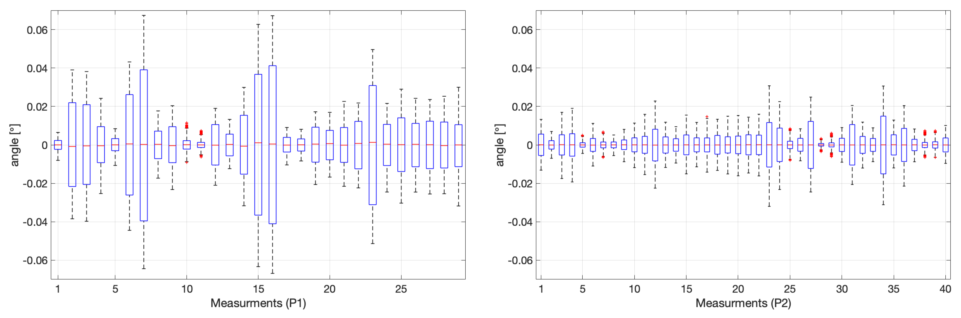
The deployment of the Qualisys motion capturing system brings an additional benefit for models, which are investigated in the wave and current tank and are thus typically already fitted with the necessary markers. Based on this the centre of gravity can be measured with a high accuracy in relation to the rigid body definition. For this current paper the swing itself is in the focus and hence additional markers are placed on the structure. The aim of the comparison is to provide an independent verification of the inclinometer and capture oscillations which are too fast for the instrument. A synchronisation of both systems was not conducted with a trigger signal but started manually at the same time, which is acceptable for the specific application. The comparison of the two instruments showed that the difference between the two measured inclination angles is smaller than or in the range of the remaining observed oscillation of the angle in a close to steady position of the swing.

2.3. Measurement Procedure

The swing itself is made of aluminium and has a mass of around 42 kg. This allows it to be safely handled by two trained persons and the crane is not needed. A pallet cart can be used for the installation at the pivot axis at P1 as shown in Figure 1d. For both of the different pivot axis options, shown in Figure 1 and Figure 2, the swing rests on two cutting edges on top of the support structure, which only requires a very small adjustment. As part of the initial installation as well as after each change of the pivot axis, the inertial inclinometer is moved so that it is orientated parallel to the pivot axis. These measurements and the following adjustments ensure that the swing sits level on the support structure. After this, the instrument is brought back to the position shown in Figure 1a to measure the angle around the pivot axis P1 or P2. It is placed on the level P0 (Figure 2) aligned to the side of the swing. After the exact positioning of the device on this plane to reach an initial measurement close to 0$°$, it is secured with electrical tape to ensure that it stayed in place. With this, the swing is ready for use.

The specific construction allows for lifting of bigger models into the swing with the crane or investigation of taller models, for example, the floating wind turbine model which can be seen in the background of Figure 1a. The width is limited to 1.3 m; and the other dimensions do not have a hard limit [30]. Ideally, the investigated model is placed so that the swing stays in the zero position, which might be difficult to achieve for a heavier model. This can be corrected with an offset in the calculations introduced in Section 2.4.

The next steps are dependent on the purpose of the investigation but, typically, the centre of gravity (CG) has to be measured first. Therefore, a rope is attached on the cross profile of the swing, which holds the relevant pivot axis at a distance of 0 to 0.65 m. This rope holds the hanger for the calibration weight. The smallest step used here is 50 g. After loading the swing or changing the mass, the oscillation of the swing is damped with the two finger tips of the operating person to introduce a certain amount of damping to achieve a new equilibrium faster. The angle is measured for typically 64 s to ensure that the magnitude of the remaining oscillation was captured and can be averaged out. This is followed by a further change of the mass until the maximum range of 3$°$ is reached. Control measurements with at least one additional distance between rope and pivot axis are advisable. This ensures that potential user errors can be detected. The calculation of the CG is introduced in Section 2.4 and Section 3.1 presents the results for the empty swing which is expanded for an example model in Section 3.2.

The distance of the CG as well as the mass of the object are a constant value and, by oscillating around a point/an axis, the moment of inertia (MI) can be calculated, knowing the period of the oscillation. Section 2.4 provides the requisite mathematical background and Section 3.3 compares the measurement of the empty swing with the theoretical values. For the presented experimental set-up, the initial inclination should be limited to $\pm 3°$ based on the range of the inertial inclinometer. If the changes are too fast, the reading of the instrument is not correct and underestimates the actual angles. This is to be expected given that the device is designed for high accuracy measurements of slow changing objects. The limitations were reached for oscillations around the pivot axis P2. In those cases, the motion capturing system can provide the observation and check with a stopwatch allows a further independent verification.

2.4. Basic Equations

Two different sets of equations are needed to calculate the centre of gravity (CG) as well as the moments of inertia (MI). The location of CG is based on steady measurements of an inclined swing due to added calibration weights. Knowing this value allows for the calculation of the MI based on the period or frequency of an oscillating system. The presented experimental set-up enabled measurements to be conducted with two different pivot points, but is limited to one direction at a time.

For the calculation of the CG, the starting point is Newton’s first law and the assumption that the system is in equilibrium and not moving. A zero acceleration results in a zero sum of forces in all directions. Furthermore, it can be assumed that the system can be reduced to a two-dimensional problem, hence all imbalances along the pivot axis are absorbed by the small changes in the reacting forces at the blade edges. Ideally, each side holds half of the sum of the mass of the swing $F_S$, the additional model $F_M$ as well as the additional calibration weights $F_{W,i}$. The latter is applied to incline the swing with an angle of ${\alpha }_i$. The purpose of the following equations is to connect the individual forces F and distances or levers d based on i measurements with different $F_{W,i}$ at $d_{W,i}$. 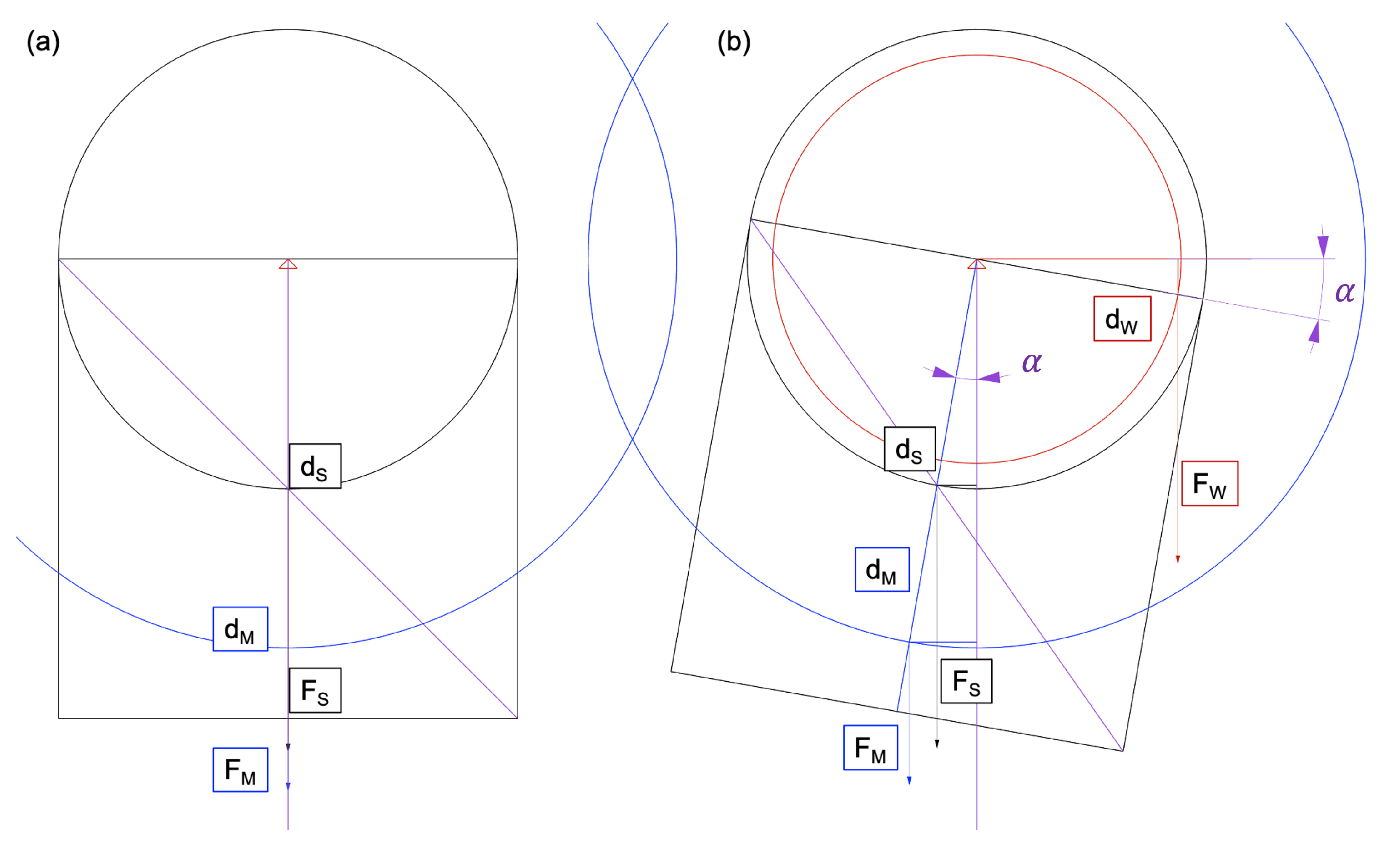To connect those, the moment balance of one example configuration is investigated in Figure 3. In this example a large angle $\alpha$ of 10$°$ is applied and the distances of the chosen to be easily identifiable.

The sum of the moments/torques around the pivot point (red triangle in Figure 3) can be calculated based on the following equation:

$$\sum M=0=F_W{d}_{W}cos\left(\alpha \right)-\left(F_S{d}_S+F_M{d}_M\right)sin\left(\alpha \right)$$

(1)

All forces in this equation are known by weighting the model as well as the swing and for the additional $F_W$ specific calibration weights are used. The distances $d_S$ and $d_M$ describe the distance of the pivot centre to the centre of gravity of the swing or the model, respectively. The distance $d_W$ is also constant and predefined. By using the solution with the rope, the added force always acts at the same point and with a fixed distance to the pivot point. Alternatively, the calibration weights could be placed on the swing but in this particular case, the specific location of the CG for the masses has to be calculated, which could also result in inaccuracies. Furthermore, the angle $\alpha$ is the key output of the measurement and can be calculated based on the following equation:

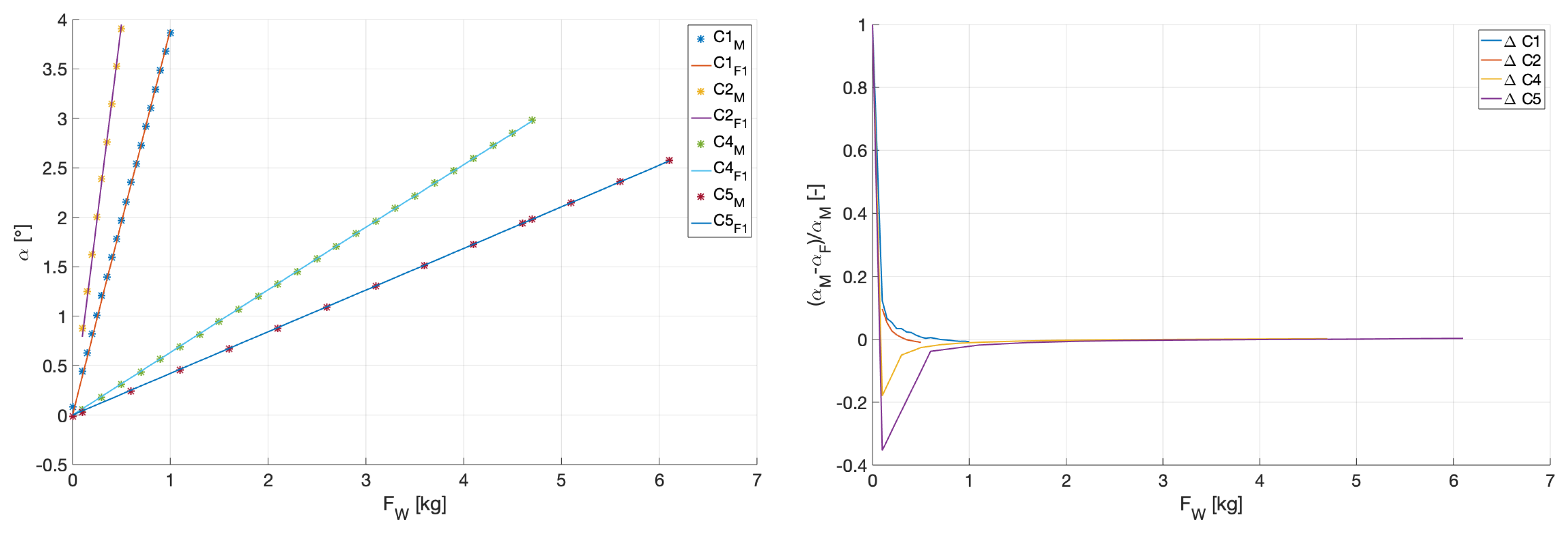
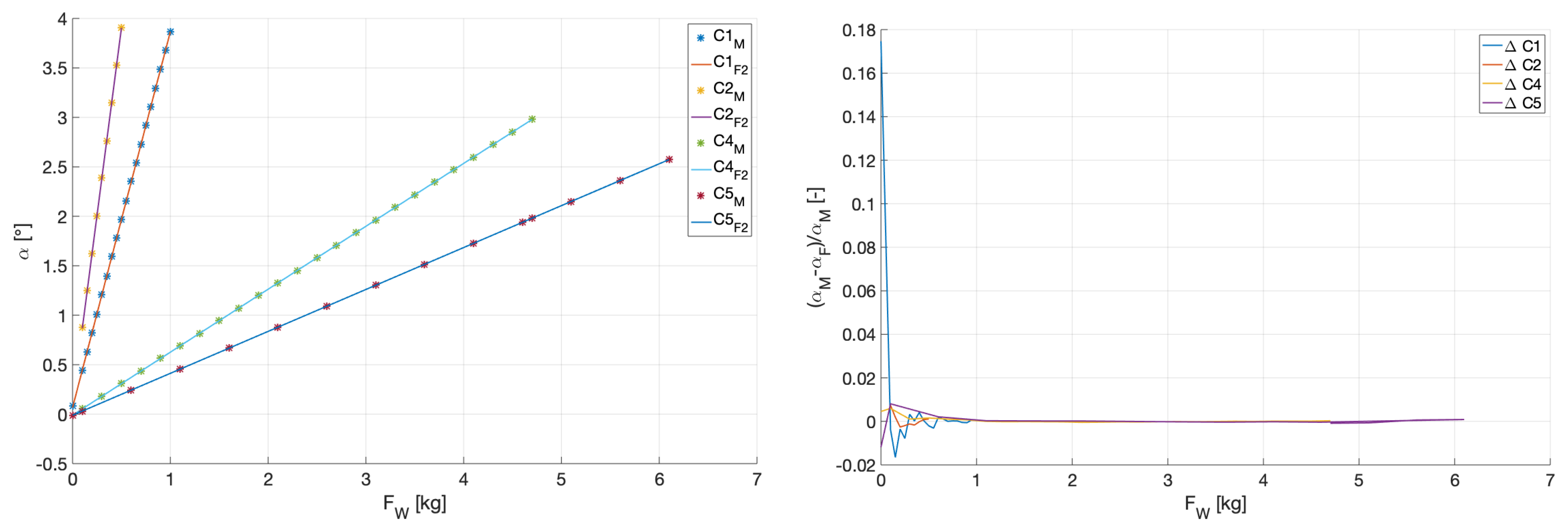
$$tan\left(\alpha \right)=\frac{sin\left(\alpha \right)}{cos\left(\alpha \right)}=\frac{F_W{d}_W}{F_S{d}_S+F_M{d}_M}$$

(2)

The distance $d_M$ should be the only unknown for future applications, which can fitted to a point cloud of different additional masses $F_W$ at difference distances $d_W$. Therefore, the swing is analysed without an additional model ($F_W=d_W=0$) and the distance $d_S$ representing the distance between the CG of the swing to the pivot point can be calculated based on the following equation:

$$d_S=\frac{F_W{d}_W}{F_S\tan \left(\alpha \right)}$$

(3)

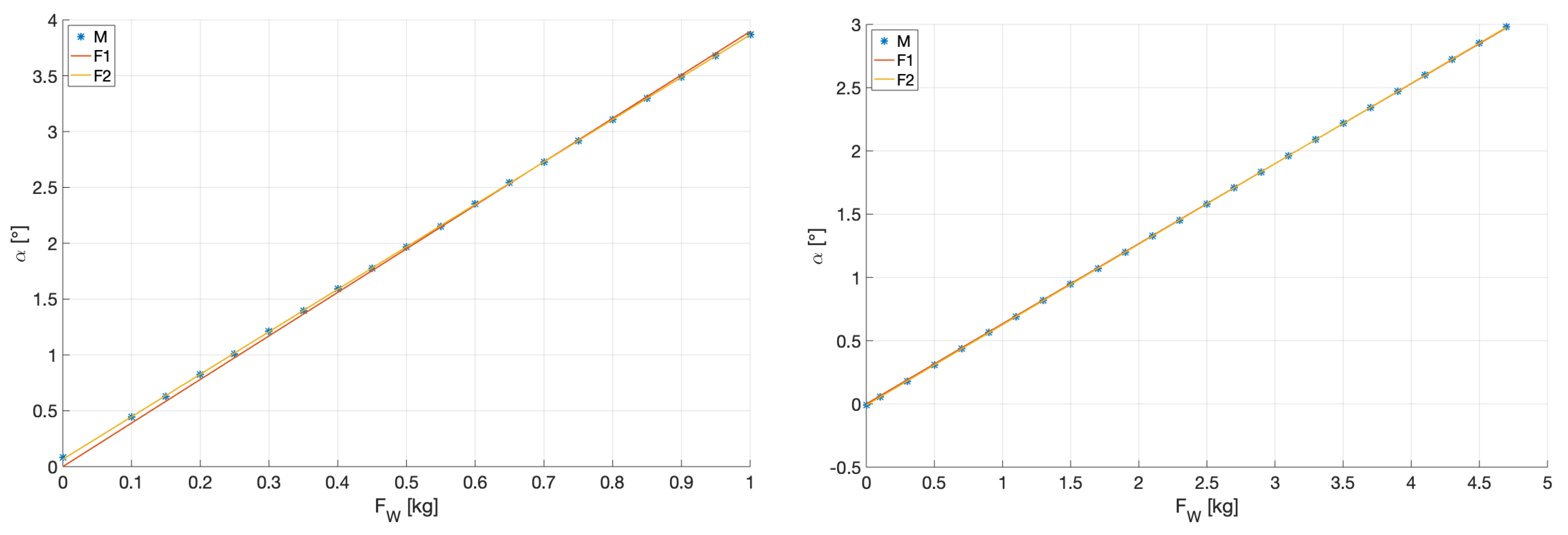
This equation is utilised and further investigated in Section 3.1 based on measurements of a stable new equilibrium of the swing due the additional calibration weights. In a second step, the moment of inertia (MI) is evaluated based on the period of an oscillating swing based on the following equation for a free oscillating pendulum around a horizontal axis [1]:

$$T=2\pi \sqrt{\frac{I_P}{mgR}}\to I_P=\frac{T^2}{4{\pi }^2}mgR$$

(4)

The variable $I_P$, representing the MI around the pivot axis, can be calculated based on the period of the oscillation T, the mass of the rigid body m, the constant gravity acceleration g and the distance R (length between the pivot point and the CG), which is equal to $d_S$ from the previous CG calculation. The period T of a damped oscillation can be evaluated based on:

$$y\left(t\right)=\alpha \left(t\right)=A{e}^{-\lambda t}cos\left(\frac{2\pi t}{T}+\varphi \right)\to T=2\pi t{\left(arccos\left(\frac{\alpha }{A{e}^{-\lambda t}}\right)-\varphi \right)}^{-1}$$

(5)

In this case, the time depending amplitude $y\left(t\right)$ is identical to the measured angle $\alpha$. t represents the time. The oscillation starts with the initial amplitude A. Two further constants $\lambda$ and $\varphi$ represent the decay constant and the phase angle. The dynamic measurement provides a time series of angles $\alpha$ in relation to the time vector t, which can be used to fit Equation (5). For the further analysis, only the time period T is needed and all other constants can be used as control values.

The resulting moment of inertia output based on Equation (4) is referenced around the pivot point and, to compare both pivot axes, the parallel axis theorem is used to calculate the MI around the centre of gravity I in relation to the $I_P$, mass m and distance $d_S$ as following:

$$I_P=I+m{d}_S^2\to I=I_{P1}-m{d}_{SP1}^2=I_{P2}-m{d}_{SP2}^2$$

(6)

This connection is further used to calculate the MI of the empty swing (Section 3.3). The specific MI around the two different pivot points are important for the further usage of this experimental set-up to evaluate the MI of added model $I_M$. The connection is shown in Equation (7) for the pivot point P1 and can be transformed to alternative reference points based on the parallel axis theorem Equation (6).

$$I_{P1mes}=\frac{T^2}{4{\pi }^2}(m_S+m_M)g{d}_{Smes}=I_{P1}+I_{MP1}$$

(7)

The presented equations for the calculation of the individual vales for CG as well as the MI are further used to analyse the conducted measurements. All those analyses are conducted with the software MATLAB.

3. Results

3.1. Centre of Gravity (CG)—Swing

In this first step, the swing is investigated without an additional model on it. Consequently, Equation (2) is simplified to Equation (3), hence $F_M$ is equal to zero. Calibration weights $F_W$ are added in different distances $d_W$ utilising both pivot axes (Figure 2).

Table 2. Overview of the investigated cases and the calculated distance of the CG based on the two different fitting functions $SwingF1$ and $SwingF2$—mean values for both pivot axis P1 and P2 presented in Table 3.

Case	${\mathit{d}}_{\mathit{W}}$	Max ${\mathit{F}}_{\mathit{W}}$	Max i	Pivot Point	${\mathit{d}}_{\mathit{SF}1}$	${\mathit{d}}_{\mathit{SF}1}$-Mean(${\mathit{d}}_{\mathit{SF}1}$)	${\mathit{d}}_{\mathit{F}2}$(1) = ${\mathit{d}}_{\mathit{SF}2}$	${\mathit{d}}_{\mathit{F}2}$(2)	${\mathit{d}}_{\mathit{SF}2}$-Mean(${\mathit{d}}_{\mathit{SF}2}$)
	(m)	(kg)			(mm)	(mm)	(mm)	($°$)	(mm)
C1	0.2	1.0	20	P1	69.6	0.47	71.3	0.0011	0.07
C2	0.4	0.5	9	P1	68.6	−0.57	71.3	0.0019	0.03
C3	= C1 + C2		29	P1	69.2	0.10	71.2	0.0013	−0.10
C4	0.6	4.7	25	P2	1283.9	−0.33	1277.4	−0.0002	0.73
C5	0.4	6.1	15	P2	1283.9	−0.35	1274.9	−0.0003	−1.76
C6	= C4 + C5		40	P2	1284.9	0.68	1277.7	−0.0002	1.03

provides an overview of the conducted measurements with the empty swing and the specification of the analysis cases.

All individual measurements are analysed in Figure 4 for the case C3 and C6, which include both distances for each pivot point. The biggest differences in the individually recorded time series from the mean value are in the range of 0.06$°$ for P1 and 0.03$°$ for P2. Both values are significantly larger than the non-linearity and non-repeatability of the inertial inclinometer. Adding the normalised minimum and maximum (Figure 4), as well as looking at the time series in detail, shows that a small oscillation could still be found. The effect of this can be minimised by using an time average for the fitting of the equation. Therefore, only the last 54 of the total captured 64 s are used. This limits the influence of disturbances introduced by the swing operator. The solution of the curve-fitting is implemented with the MATLAB function lsqcurvefit in least-squares sense. This needs as inputs a function $SwingF1$ based on Equation (3), initial point $d0F1$, input data $xData$ (vector with the used calibration weights $FW$) as well as the connected distances $distanceW$ (equal to $d_W$) and observed output $yData$ (equal to $\alpha$). The measured angle $\alpha$ are in deg and have to be transformed to radians. A reduced MATLAB code is presented in the following equations:

$$\begin{array}{c}\hfill SwingF1=@(d,xData)xData.\ast distanceW./(FS\ast d);\end{array}$$

(8)

$$\begin{array}{c}\hfill dSF1=lsqcurvefit(Swing,d0F1,FW,tan(yData./180.\ast pi\left)\right);\end{array}$$

(9)

The initial values for the distance was chosen based on the following equation:

$$\begin{array}{c}\hfill d0F1=\left\{\begin{array}{cc}0.1\ast fac,\hfill & \mathrm{for}\mathrm{P}1\left[\mathrm{m}\right],\hfill \\ 1.255\ast fac,\hfill & \mathrm{for}\mathrm{P}2\left[\mathrm{m}\right].\hfill \end{array}\right.\end{array}$$

(10)

The initial point $d0F1$ is set close to the expected distance $d_S$ but this assumption has been altered by a factor $fac$ in the range of 0.1 to 10 to ensure that the result is independent of this first estimate [34,35]. Table 2 summarises the results for all analysis cases and indicates that the difference of the individual fittings are in the range of 0.5 mm of the average value for each pivot axis. The addition $F1$ indicates that the values are referencing the initial Equation (3). Figure 5 focuses on the four individual measurement series and presents the direct comparison of measurement M and fitted data F. The standardised difference between those two values shows that especially around $F_W$ = 0 kg, the fitting has comparable big deviations. This is caused by the fact that the swing was not in a perfect zero position at the beginning of the measurement. As an improvement, a second function $SwingF2$ is defined, which allows a constant offset:

$$\begin{array}{c}\hfill SwingF2=@(d,xData)xData.\ast distanceW./(FS\ast d(1\left)\right)+d\left(2\right);\end{array}$$

(11)

$$\begin{array}{c}\hfill dSF2=lsqcurvefit(Swing,d0F2,FW,tan(yData./180.\ast pi\left)\right);\end{array}$$

(12)

In this case, two initial values have to be chosen:

$$\begin{array}{c}\hfill d0F2=\left\{\begin{array}{cc}[0.1,0].\ast fac,\hfill & \mathrm{for}\mathrm{P}1\left[\mathrm{m}\right],\hfill \\ [1.255,0].\ast fac,\hfill & \mathrm{for}\mathrm{P}2\left[\mathrm{m}\right].\hfill \end{array}\right.\end{array}$$

(13)

Figure 6 presents the results for the fitting based on the $SwingF2$. The differences show a comparable distribution as for the fitting with $SwingF1$ but the normalised value reduces drastically from 1 to smaller 0.18. Two examples, namely for the analysis cases C1 and C4, are provided in Figure 7. The value for $F_W$ = 0 kg is a strong indicator how good the fitting with the original function $SwingF1$ performs.

Table 2 summarises the chosen analysis cases as well as the results based on both fitting functions $SwingF1$ (indicated with $F1$) and $SwingF2$, which introduces a constant offset $d_{F2}\left(2\right)$. The values are in the range of 10${}^{-3}$ degrees. A detailed comparison of the mean values for each of the functions is presented in

Table 3. Comparison of the theoretical values and the fitted distances $d_S$ based on the function $SwingF1$ and $SwingF2$ for both pivot axis P1 and P2 as well as the distance between P1 and P2.

	${\mathit{d}}_{\mathit{Stheo}}$	${\mathit{d}}_{\mathit{SF}1}$	${\mathit{d}}_{\mathit{SF}2}$	${\mathit{d}}_{\mathit{SF}1}$-${\mathit{d}}_{\mathit{SF}2}$	${\mathit{d}}_{\mathit{SF}1}$-${\mathit{d}}_{\mathit{Stheo}}$	${\mathit{d}}_{\mathit{SF}2}$-${\mathit{d}}_{\mathit{Stheo}}$	(${\mathit{d}}_{\mathit{SF}1}$-${\mathit{d}}_{\mathit{Stheo}}$)/${\mathit{d}}_{\mathit{Stheo}}$	(${\mathit{d}}_{\mathit{SF}2}$-${\mathit{d}}_{\mathit{Stheo}}$)/${\mathit{d}}_{\mathit{Stheo}}$
	(mm)	(mm)	(mm)	(mm)	(mm)	(mm)	(%)	(%)
P1	71.9	69.1	71.3	−2.1	−2.7	−0.6	−3.81%	−0.82%
P2	1271.9	1284.2	1276.7	7.6	12.4	4.8	0.97%	0.38%
P2-P1	1200.0	1215.1	1205.4	9.7	15.1	5.4	1.26%	0.45%

. The difference between the results of $d_S$ based on the functions show that the difference is in the range of millimetres. An under-prediction of the theoretical approach is expected because those calculations are conducted without the inertia inclinometer and the attached cable. The difference between the two distances is for the fitting with the function $SwingF2$ closer to the theoretical values. Furthermore, Figure 7 shows the advantage of this adapted function for small errors around the zero value. Based on those points, the function $SwingF2$ can be seen as better suited for future analysis. Nevertheless, further measurements have to be conducted to improve the evaluation of the CG of the swing.

3.2. Centre of Gravity (CG)—Example

The centre of gravity (CG) for the swing is investigated in Section 3.1 based on Equation (3). In a next step, an example model is investigated, which is part of a research project at FloWave. Figure 8 shows this part of a floating structure, which is based on a hexagonal ground with a side length of 280 mm and a total height of 277 mm. The wall and bottom thickness is 12 mm. The total mass of the structure is 11.27 kg and the theoretical CG lays in the centre in the height of 100.273 mm in relation to the bottom. This example was chosen because it has a typical size and comparable simple geometry for which the theoretical value should be very accurate.

Table 4. Overview of the investigated cases for the example geometry presented in Figure 7—Data fitted based on Equation (2) similarly to the approach shown in Equation (11).

Case	${\mathit{d}}_{\mathit{W}}$	Max ${\mathit{F}}_{\mathit{W}}$	Max i	Pivot	${\mathit{d}}_{\mathit{MP}1}$	${\mathit{d}}_{\mathit{MP}1}$-Mean(${\mathit{d}}_{\mathit{MP}1}$)	d(2)	${\mathit{d}}_{\mathit{MP}0}$	${\mathit{d}}_{\mathit{MP}0}$-${\mathit{d}}_{\mathit{Mtheo}}$	(${\mathit{d}}_{\mathit{MP}0}$-${\mathit{d}}_{\mathit{Mtheo}}$)/${\mathit{d}}_{\mathit{Mtheo}}$
	(m)	(kg)		Point	(mm)	(mm)	($°$)	(mm)	(mm)	(%)
C1	0.64	1.0	17	P1	837.6	2.1	−0.00039	100.4	0.1	0.11%
C2	0.40	1.0	11	P1	829.3	−6.3	−0.00036	108.7	8.4	8.42%
C3	0.20	1.1	6	P1	838.8	3.2	−0.00043	99.3	−1.0	−1.02%
C4	∑		34	P1	836.6	1.0	−0.00037	101.4	1.2	1.17%
Mean					835.6	0.0		102.5	2.2	2.17%

provides an overview of the conducted three measurement series with three different distances $d_W$ of the added calibration weights. The analysis base on Equation (2) but also includes the additional constant offset, which was introduced in Equation (11). This value $d\left(2\right)$ is relatively small (range of ${10}^{-4}$ degrees) but allows a far better fitting result. Two of the three measurement series provide a very good agreement but the C2 series is not as good. A detailed investigation of the individual time series do not indicate any obvious mistake as well as the analysis similar to Figure 4. This leads to the conclusion that a single measurement series with only one distance $d_W$ is not enough and can potentially lead to an error, which is hard to identify. The guidance should be to use multiple distances for the added calibration weights.

3.3. Moment of Inertia (MI)

The previous measurement of the centre of gravity based on different new stable equilibria caused by different added calibration weights. Instead of this stable conditions, the oscillating system is observed for the calculation of the moment of inertia (MI) based on Equation (4). The required input of the oscillation is the period T, which is calculated based on the following approaches:

• F1: simple cosine oscillation assuming a simple harmonic oscillator without the consideration of damping;
• F2: damped harmonic oscillator based on Equation (5);
• F3: similar to F2 but the length of the measurement is limited to a full period;
• F4: similar to F2 but a constant value is added similar to the approach shown in Equation (11).

The empty swing is observed three times for each of the two pivot points P1 and P2 (Figure 2). Each capture time is at least 160 s. For the higher pivot point P2, the oscillation is too fast for the inertial inclinometer and the results from the Qualisys motion capturing system are used. As mentioned in Section 2.2, both systems capture the angle $\alpha$ with a measurement frequency of 256 Hz.

Table 5. Results for the oscillation around P2 for the four different functions to calculate the period T, initial amplitude A, phase angle $\varphi$ and decay constant $\lambda$ for three different runs (repeats)—offset for F4 is −0.014,−0.014 and −0.007 $°$.

	Run 1				Run 2				Run 3
	${\mathit{T}}_{\mathit{P}2\mathit{R}1}$	abs(A)	$\mathit{\varphi }$	$\mathit{\lambda }$	${\mathit{T}}_{\mathit{P}2\mathit{R}2}$	abs(A)	$\mathit{\varphi }$	$\mathit{\lambda }$	${\mathit{T}}_{\mathit{P}2\mathit{R}3}$	abs(A)	$\mathit{\varphi }$	$\mathit{\lambda }$
F1	2.8455	2.816	1.111	not used	2.8461	3.418	−1.398	not used	2.8462	3.693	−0.086	not used
F2	2.8455	3.495	1.110	0.00299	2.8460	4.306	−1.399	0.00321	2.8463	4.710	−0.083	0.00339
F3	2.8455	3.494	1.110	0.00299	2.8460	4.303	−1.400	0.00320	2.8463	4.707	−0.084	0.00338
F4	2.8455	3.495	1.110	0.00299	2.8460	4.307	−1.399	0.00321	2.8463	4.710	−0.083	0.00338

results for the higher pivot point P2 and

Table 6. Results for the oscillation around P1 for the four different functions to calculate the period T, initial amplitude A, phase angle $\varphi$ and decay constant $\lambda$ for three different runs (repeats)—offset for F4 is 0.0004, 0.0012 and −0.0022$°$.

	Run 1				Run 2				Run 3
	${\mathit{T}}_{\mathit{P}1\mathit{R}1}$	abs(A)	$\mathit{\varphi }$	$\mathit{\lambda }$	${\mathit{T}}_{\mathit{P}1\mathit{R}2}$	abs(A)	$\mathit{\varphi }$	$\mathit{\lambda }$	${\mathit{T}}_{\mathit{P}1\mathit{R}3}$	abs(A)	$\mathit{\varphi }$	$\mathit{\lambda }$
F1	7.3078	0.795	−0.020	not used	7.2561	0.232	1.707	not used	7.2851	0.712	−0.205	not used
F2	7.3083	1.116	−0.014	0.00480	7.2809	1.101	2.101	0.00550	7.2878	1.340	−0.172	0.00489
F3	7.3081	1.117	−0.016	0.00481	7.2800	1.103	2.082	0.00548	7.2876	1.344	−0.176	0.00490
F4	7.3083	1.116	−0.014	0.00480	7.2809	1.102	2.101	0.00550	7.2878	1.340	−0.172	0.00489

for the lower one P1. For the fitting with the simple harmonic oscillation, the decay constant $\lambda$ is not used and the initial amplitude A is smaller than for the other functions F2–F4. The latter is obvious because this fitting does not consider the reduction of the amplitude with the time and consequently delivers an average amplitude over the observation time. All other values are very stable and largely independent of the used fitting function. The period T is compared in detail in

Table 7. Comparison of the calculated periods T based on the four different functions and for the three runs R1, R2 and R3—the presented differences represents the values minus the average over all three runs of the period based on F2-all values in Seconds.

	P2			P1			P2			B
	${\mathit{T}}_{\mathit{P}\mathbf{2}\mathit{R}\mathbf{1}}$	${\mathit{T}}_{\mathit{P}\mathbf{2}\mathit{R}\mathbf{2}}$	${\mathit{T}}_{\mathit{P}\mathbf{2}\mathit{R}\mathbf{3}}$	${\mathit{T}}_{\mathit{P}\mathbf{1}\mathit{R}\mathbf{1}}$	${\mathit{T}}_{\mathit{P}\mathbf{1}\mathit{R}\mathbf{2}}$	${\mathit{T}}_{\mathit{P}\mathbf{1}\mathit{R}\mathbf{3}}$	$\mathbf{\Delta }{\mathit{T}}_{\mathit{P}\mathbf{2}\mathit{R}\mathbf{1}}$	$\mathbf{\Delta }{\mathit{T}}_{\mathit{P}\mathbf{2}\mathit{R}\mathbf{2}}$	$\mathbf{\Delta }{\mathit{T}}_{\mathit{P}\mathbf{2}\mathit{R}\mathbf{3}}$	$\mathbf{\Delta }{\mathit{T}}_{\mathit{P}\mathbf{1}\mathit{R}\mathbf{1}}$	$\mathbf{\Delta }{\mathit{T}}_{\mathit{P}\mathbf{1}\mathit{R}\mathbf{2}}$	$\mathbf{\Delta }{\mathit{T}}_{\mathit{P}\mathbf{1}\mathit{R}\mathbf{3}}$
F1	2.8455	2.8461	2.8462	7.3078	7.2561	7.2851	−0.0004	0.0001	0.0003	0.0155	−0.0362	−0.0072
F2	2.8455	2.8460	2.8463	7.3083	7.2809	7.2878	−0.0004	0.0001	0.0003	0.0159	−0.0114	−0.0045
F3	2.8455	2.8460	2.8463	7.3081	7.2800	7.2876	−0.0004	0.0001	0.0003	0.0157	−0.0123	−0.0047
F4	2.8455	2.8460	2.8463	7.3083	7.2809	7.2878	−0.0004	0.0001	0.0003	0.0159	−0.0114	−0.0045

. This table also includes the difference with the averaged value for the period T for each P1 (7.2923 s) and P2 (2.8460 s). The maximum difference is 0.0159 s. Consequently, it can be summarised that the fitting results for the period of the oscillation T are largely independent of the chosen fitting function $F1$ to $F4$.

Equation (4) introduces the connection between the constants and the values, which are depending on the specific pivot points. Those are the period T and the distance R. The latter is equal to the distance $d_S$ evaluated in Section 3.1.

Table 8. Analysis of the results for the measurements for the moment of inertia for the empty swing—two different investigated pivot points P1 and P2—comparison to the theoretical values provided in Table 1.

	T	$\mathit{R}=\mathit{ds}$	${\mathit{I}}_{\mathit{Pcalc}}$	I	${\mathit{I}}_{\mathit{P}1}$	${\mathit{I}}_{\mathit{P}2}$	${\mathit{I}}_{\mathit{P}1}$-${\mathit{I}}_{\mathit{P}1\mathit{theo}}$	${\mathit{I}}_{\mathit{P}2}$-${\mathit{I}}_{\mathit{P}2\mathit{theo}}$	$\mathbf{\Delta }{\mathit{I}}_{\mathit{P}1}$/${\mathit{I}}_{\mathit{P}1\mathit{theo}}$	$\mathbf{\Delta }{\mathit{I}}_{\mathit{P}2}$/${\mathit{I}}_{\mathit{P}2\mathit{theo}}$
	(s)	(m)	(kg m${}^2$)	(kg m${}^2$)	(kg m${}^2$)	(kg m${}^2$)	(kg m${}^2$)	(kg m${}^2$)	(%)	(%)
P1	7.2923	0.071	39.818	39.603	39.818	108.517	0.073	0.622	0.18%	0.58%
P2	2.8460	1.277	108.639	39.726	39.941	108.639	0.196	0.745	0.49%	0.69%
Diff	4.4464	−1.205	−68.821	−0.123	−0.123	−0.123
theo					39.745	107.895

summarises the input values and the calculation based on basic Equation (4) with a mass m of 42.280 kg and g equal 9.81 m s${}^{-2}$. This value is called $I_{Pcalc}$ and has as a reference point the individual pivot point P1 or P2. A comparison is possible by calculating the moment of inertia I around the CG based on Equation (6). The similar approach is used to calculate the MI for both pivot axis based on the individual measurement (one is measured and the other is calculated), which can be compared directly to the values calculated based on the theoretical approach (Table 1). The difference between the theoretical value and the measured are small and within an acceptable range. Doniselli et al. [6] report an error of less than 3% and specify this as a very good result.

Noticeable also is that the difference between both measurements corrected for a similar pivot point results in the exact same difference of −0.12253 kg m${}^2$. This is in addition to the discrepancy in the distance between the backward calculated distance between P1 and P2 (should be exactly 120 mm, Figure 2), which indicates that a systematic error occurs. A first assumption is that the inclinometer has to be placed further away on P0 to achieve an initial equilibrium for the measurements with the higher pivot point P2. In future optimisation investigations, the inclinometer could be left at the same location needed for the pivot point P1 and an offset accepted. Based on such a measurement, the influence of the exact location of the instrument could be investigated. Alternatively, the location of the pivot points can be further tuned to reduce this offset. This is part of ongoing work.

4. Discussion

Based on the initial tests of the empty swing as well as different client testing, the design concept has proven to be very useful and accurate. The aim for the design was to bring the CG of the swing as close as possible to the pivot point P1. With a distance of only a little more than 70 mm (Table 3), this can be seen as achieved and the extremely long free oscillation of the swing proves this. The swings remain safe for manual handling of even heavier models on it. A maximum capacity was not yet specified and will require further analysis. Due to the crane accessibility, the top of the swing is open leading to a U-shape of the structure. In very rare occasions—mainly when changing the pivot points—it could be observed that the swing starts to vibrate (comparable to the oscillation of a tuning fork) and the measurement has to be paused to allow a damping of this. This happens only on very rare occasions and can be prevented by a careful handling of the swing. Bracing at the top of the structure, which could be removable, might have been a better option and could be an improvement for a future design of a comparable swing. The blade edge is identified as a potential risk when changing the position of the swing. This danger can be substantially reduced by handling with a pallet truck or by handling with at least two trained persons. The support frames that are split into two and the swing allow for space-saving storage as well as easy and flexible handling. Nevertheless, the mass of the structure and the expanded footprint ensure a stable seating for the knife edge of the swing. There would also be the option to deploy the complete structure for measurements in submerged conditions, which can be easily realised by placing the swing on the raisable floor in the centre of the wave and current tank FloWave.

The main instrument for the experimental set-up is the inertia inclinometer with a range of ±3$°$. It provides the angle of the movable swing with a very high precision and the only downside is that it is not capable to follow fast oscillations, which is not a specification for the typical application of this device. Nevertheless, those specific measurements can be covered with the motion capturing system bringing the additional benefit that the measurements are directly connected to the rigid body definition used in the wave tank. In future, a simple light switch could be added to capture the zero passing of the swing. For masses over 20 kg, crane scales (or similar) have to be used, which are typically of lower precision than the bench scales. Hence, a further improvement is to expand the available range of scales.

A great benefit of this experimental set-up is to provide the distance of the centre of gravity with a very high accuracy in a standardised and repeatable way. Furthermore, the dynamic tests on the swing replace previous measurements hanging from a pivot point on the ceiling. It is indisputable that a more complex measurement including multiple load cells is able to quantify the full location of the centre of gravity and the moments of inertia also with a high accuracy and in less time [1]. The presented swing has a clear limitation to one degree of freedom for the oscillation, as well as a simple, stable and repeatable positioning of the model in relation to the pivot axis. Nevertheless, it is a good compromise providing an accurate and standardised measurement, which is suitable for the typical projects investigated at FloWave. The main aim is to provide a standardised measurement, which can be used not only as a simple check of the theoretical value based on CAD but also to provide a very high accuracy for the moment of inertia, which can be included in the analysis of the results from the wave and current tank.

5. Conclusions

The quantification of the location of the centre of gravity (CG) as well as the moments of inertia (MI) are critical for many investigations. In the case of tank testing, the majority of investigated floating devices are downscaled models. Due to constraints connected with the model build as well as the ballasting, the precise realisation of the CG as well as the MI have a higher uncertainty connected. Hence, it is very important to measure those values very precisely at model scale to check and potentially correct the connected numerical simulations and empirical analysis. Different methods could be used and, in this paper, an experimental set-up for a swing is presented and investigated. The swing is balanced on two knife edges placed on a support structure, which reduces the potential motion to a single rotation around a pivot axis. It allows static investigations to measure the distance of the CG in the range of millimetres as well as dynamic investigations for the additional calculation of the MI in the range of 1%. Therefore, two different pivot points are available, and it could be shown that a multi distance check with the calibration weights are very important to ensure the quality of the measurement. The theoretical analyses are expanded with a constant offset to compensate imperfection in the zeroing of the swing. A removable bracing at the top, which provides stability but can be removed to ensure crane accessibility, was identified as a potential improvements of the design. All in all, the swing provides a flexible and standardised experimental set-up for static and dynamic investigations to quantify the centre of gravity and moments of inertia of typical models tested in FloWave.

References

1. Schedlinski, C.; Link, M. A survey of current inertia parameter identification methods. Mech. Syst. Signal Process. 2001, 15, 189–211. [Google Scholar] [CrossRef]
2. Mondal, N.; Acharyya, S.; Saha, R.; Sanyal, D.; Majumdar, K. Optimum design of mounting components of a mass property measurement system. Measurement 2016, 78, 309–321. [Google Scholar] [CrossRef]
3. Zhang, L.S.; Wang, M.B.; Lin, J.J.; Liul, P. A demodulation algorithm for processing rotational inertia signals using a torsion pendulum method based on differentiation and resonance frequency analysis. Meas. Sci. Technol. 2021, 32, 025005. [Google Scholar] [CrossRef]
4. Olmedo, N.A.; Barczyk, M.; Lipsett, M. Experimental determination of the inertial properties of small robotic systems using a torsion platform. Mech. Syst. Signal Process. 2019, 131, 71–96. [Google Scholar] [CrossRef]
5. Brancati, R.; Russo, R.; Savino, S. Method and equipment for inertia parameter identification. Mech. Syst. Signal Process. 2010, 24, 29–40. [Google Scholar] [CrossRef]
6. Doniselli, C.; Gobbi, M.; Mastinu, G. Measuring the inertia tensor of vehicles. Veh. Syst. Dyn. Int. J. Veh. Mech. Mobil. 2002, 37, 301–313. [Google Scholar] [CrossRef]
7. Previati, G.; Gobbi, M.; Mastinu, G. Measurement of the mass properties of rigid bodies by means of multi-filar pendulums—Influence of test rig flexibility. Mech. Syst. Signal Process. 2019, 121, 31–43. [Google Scholar] [CrossRef]
8. Zhu, T.; Li, F. Experimental investigation and performance analysis of inertia properties measurement for heavy truck cab. Adv. Mech. Eng. 2015. [Google Scholar] [CrossRef] [Green Version]
9. Liu, Y.; Liang, B.; Xu, W.F.; Wang, X.Q. A method for measuring the inertia properties of a rigid body using 3-URU parallel mechanism. Mech. Syst. Signal Process. 2019, 123, 174–191. [Google Scholar] [CrossRef]
10. Previati, G. Large oscillations of the trifilar pendulum: Analytical and experimental study. Mech. Mach. Theory 2021, 156, 104157. [Google Scholar] [CrossRef]
11. Li, S.; Chu, W.; Huang, X. Measurement method of aircraft barycenter based on multi posture. Sens. Rev. 2020, 40, 217–226. [Google Scholar] [CrossRef]
12. Wang, M.; Zhang, X.; Tang, W.; Wang, J. A Structure for Accurately Determining the Mass and Center of Gravity of Rigid Bodies. Appl. Sci. 2019, 9, 2532. [Google Scholar] [CrossRef] [Green Version]
13. Zhan, X.L.; Wang, M.B.; Tang, W.Y.; Wang, J. A flexible measurement technique for testing the mass and center of gravity of large-sized objects. Meas. Sci. Technol. 2020, 31, 015006. [Google Scholar] [CrossRef]
14. Suhaimi, K.; Risby, M.S.; Tan, K.S.; Syafiq, M.S.A.; Hafizi, N.M. Heavy Military Land Vehicle Mass Properties Estimation Using Hoisting and Pendulum Motion Method. Def. Sci. J. 2019, 69, 550–556. [Google Scholar]
15. Escribano-García, R.; Corral-Bobadilla, M.; Somovilla-Gómez, F.; Lostado-Lorza, R.; Ahmed, A. A Theoretical Model with Which to Safely Optimize the Configuration of Hydraulic Suspension of Modular Trailers in Special Road Transport. Appl. Sci. 2021, 11, 305. [Google Scholar] [CrossRef]
16. Chowdhury, M.; Islam, M.N.; Iqbal, M.Z.; Islam, S.; Lee, D.-H.; Kim, D.-G.; Jun, H.-J.; Chung, S.-O. Analysis of Overturning and Vibration during Field Operation of a Tractor-Mounted 4-Row Radish Collector toward Ensuring User Safety. Machines 2020, 8, 77. [Google Scholar] [CrossRef]
17. Karolius, K.B.; Vassalos, D. Weight and buoyancy is the foundation in design: Get it right. In Proceedings of the 13th International Marine Design Conference (IMDC 2018), Helsinki, Finland, 10–14 June 2018; Volume 2, pp. 727–736. [Google Scholar]
18. Kapsenberg, G.; Wandji, C.; Duz, B.; Kim, S. A Comparison of Numerical Simulations and Model Experiments on Parametric Roll in Irregular Seas. J. Mar. Sci. Eng. 2020, 8, 474. [Google Scholar] [CrossRef]
19. Gabl, R.; Davey, T.; Ingram, D.M. Roll Motion of a Water Filled Floating Cylinder—Additional Experimental Verification. Water 2020, 12, 2219. [Google Scholar] [CrossRef]
20. Qiu, S.; Ren, H.; Li, H. Computational Model for Simulation of Lifeboat Free-Fall during Its Launching from Ship in Rough Seas. J. Mar. Sci. Eng. 2020, 8, 631. [Google Scholar] [CrossRef]
21. Kosasih, K.M.A.; Suzuki, H.; Niizato, H.; Okubo, S. Demonstration Experiment and Numerical Simulation Analysis of Full-Scale Barge-Type Floating Offshore Wind Turbine. J. Mar. Sci. Eng. 2020, 8, 880. [Google Scholar] [CrossRef]
22. Woodward, M.D.; van Rijsbergen, M.; Hutchinson, K.W.; Scott, A. Uncertainty analysis procedure for the ship inclining experiment. Ocean Eng. 2016, 114, 79–86. [Google Scholar] [CrossRef] [Green Version]
23. Taylan, M. Reliability analysis of GM and KG of ships from the inclining experiment. Proc. Inst. Mech. Eng. Part J. Eng. Marit. Environ. 2020, 234, 803–809. [Google Scholar]
24. Heller, V. Scale effects in physical hydraulic engineering models. J. Hydraul. Res. 2011, 49, 293–306. [Google Scholar] [CrossRef]
25. Ingram, D.; Wallace, R.; Robinson, A.; Bryden, I. The Design and Commissioning of the First, Circular, Combined Current and Wave Test Basin. In Proceedings of the Oceans 2014 MTS/IEEE, Taipei, Taiwan, 7–10 April 2014. [Google Scholar]
26. Gabl, R.; Davey, T.; Cao, Y.; Li, Q.; Li, B.; Walker, K.L.; Giorgio-Serchi, F.; Aracri, S.; Kiprakis, A.; Stokes, A.A.; et al. Hydrodynamic Loads on a Restrained ROV under Waves and Current. Ocean. Eng. 2021, in press. [Google Scholar]
27. Gabl, R.; Davey, T.; Cao, Y.; Li, Q.; Li, B.; Walker, K.L.; Giorgio-Serchi, F.; Aracri, S.; Kiprakis, A.; Stokes, A.A.; et al. Experimental Force Data of a Restrained ROV under Waves and Current. Data 2020, 5, 57. [Google Scholar] [CrossRef]
28. Draycott, S.; Sellar, B.; Davey, T.; Noble, D.R.; Venugopal, V.; Ingram, D. Capture and Simulation of the Ocean Environment for Offshore Renewable Energy. Renew. Sust. Energ. Rev. 2019, 104, 15–29. [Google Scholar] [CrossRef]
29. Gabl, R.; Steynor, J.; Forehand, D.I.M.; Davey, T.; Bruce, T.; Ingram, D.M. Capturing the Motion of the Free Surface of a Fluid Stored within a Floating Structure. Water 2019, 11, 50. [Google Scholar] [CrossRef] [Green Version]
30. Gabl, R.; Davey, T.; Nixon, E.; Ingram, D.I. CAD Files for the Swing to Measure the Centre of Gravity and Moment of Inertia; DataShare Edinburgh [Dataset]; University of Edinburgh: Edinburgh, UK, 2021. [Google Scholar] [CrossRef]
31. Sherborne Sensors-LSOC_LSOP Inclinometer. Available online: https://www.sherbornesensors.com/wp-content/uploads/2019/08/Sherborne-Sensors-LSOC_LSOP-Inclinometer-V2.pdf (accessed on 1 June 2021).
32. Huseynov, F.; Kim, C.; OBrien, E.J.; Brownjohn, J.M.W.; Hester, D.; Chang, K.C. Bridge damage detection using rotation measurements—Experimental validation. Mech. Syst. Signal Process. 2020, 135, 106380. [Google Scholar] [CrossRef]
33. Park, H.-S.; Kim, Y.-S.; Kim, H.-J.; Choi, J.-G.; Choi, Y.-W. Optimization of the key imaging parameters for detection of microcalcifications in a newly developed digital breast tomosynthesis system. Clin. Imaging 2013, 37, 993–999. [Google Scholar] [CrossRef] [PubMed]
34. Gabl, R.; Achleitner, S.; Neuner, J.; Aufleger, M. Accuracy analysis of a physical scale model using the example of an asymmetric orifice. Flow Meas. Instrum. 2014, 36, 36–46. [Google Scholar] [CrossRef]
35. Mathworks, Matlab Help Center “Fit”. Available online: https://uk.mathworks.com/help/curvefit/fit.html (accessed on 1 June 2021).
Figure 1. Overview of the swing with support structure (1), swing (2), inclinometer (3) and masses including the rope highlighted with a red line (4) as well as the two different pivot axis (P1 and P2): (a) Balanced swing at the pivot axis P1. (b,c) Swing at the pivot axis P2 with full calibration weights (d) Support structure moved to remove the swing.
Applsci 11 05345 g001
Figure 2. Drawing of the swing (all length in mm) and different pivot axis and reverences heights P0, P1 and P2: (a,b) Axonometric projection and overview. (c) Front view and (d) top view including dimensions.
Applsci 11 05345 g002
Figure 3. Schematic visualisation of the acting forces F and distances d from the pivot point for the swing, additional model and masses: (a) empty swing, which is in balance represented by an angle α = 0 ° (b) exemplary mass added so that α = 10 ° .
Applsci 11 05345 g003
Figure 4. Boxplot analysis of the individual measurements (13,824 data points = 54 s × 256 Hz) normalised by the mean value of the measured angle α for the lower pivots axis (P1) and the higher one (P2).
Applsci 11 05345 g004
Figure 5. Function S w i n g F 1 : fitting of the points for the analysis cases C1,C2,C4,C5 and difference of the measured value indicated with M to the fitted value F normalised by the measured value—in relation to the calibration weights F W .
Applsci 11 05345 g005
Figure 6. Function S w i n g F 2 : fitting of the points for the analysis cases C1,C2,C4,C5 and difference of the measured value indicated with M to the fitted value F normalised by the measured value—in relation to the calibration weights F W .
Applsci 11 05345 g006
Figure 7. Detailed view of the fitting for the analysis case C1 (left) and C4 (right) with both functions.
Applsci 11 05345 g007
Figure 8. Example model on the swing with support structure (1), swing (2), inclinometer (3) and calibration weights including the rope highlighted with a red line (4) as well as the used pivot axis P1: (a) overview, (b) detail from the back of the swing (c) and the knife edge pivot.
Applsci 11 05345 g008