
Calibration of Finn Model and UBCSAND Model for Simplified Liquefaction Analysis Procedures


Abstract
:1. Introduction
2. Constitutive Models
2.1. Finn Model
2.2. UBCSAND Model
3. Methodology of Model Calibration
4. Results and Discussion
4.1. Finn Model
4.2. UBCSAND Model
4.3. Comparisons of Undrained Cyclic DSS Responses
5. Conclusions
- (1)
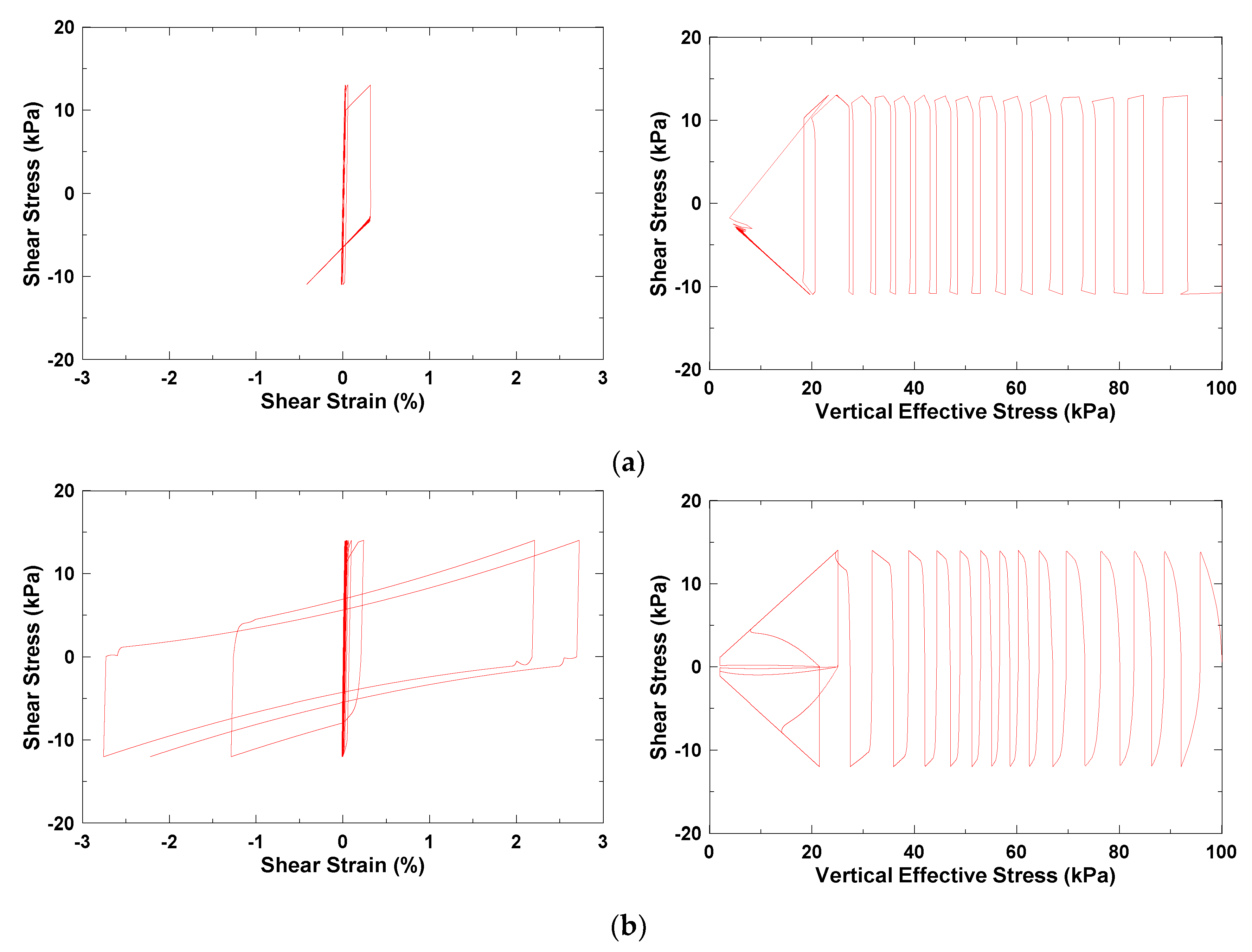
- The Finn model was not capable of modeling the banana-shaped stress–strain path and the butterfly-shaped stress path observed in the laboratory test. In contrast, the UBCSAND model could approximately capture these behaviors by tracking the stress ratio history to modify the plastic shear modulus.
- (2)
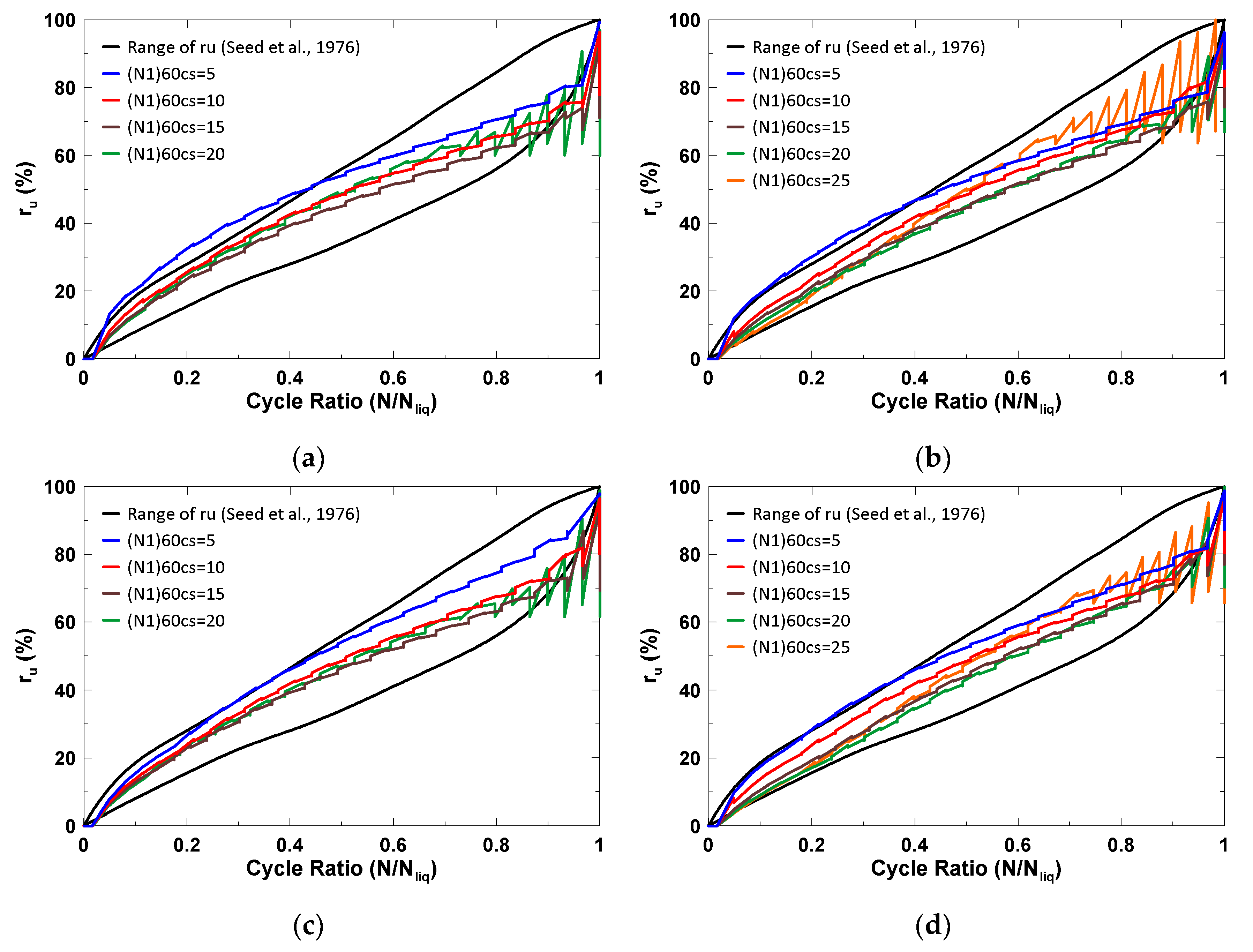
- Both models provided reasonable simulations of the excess pore pressure accumulation during cyclic loadings.
- (3)
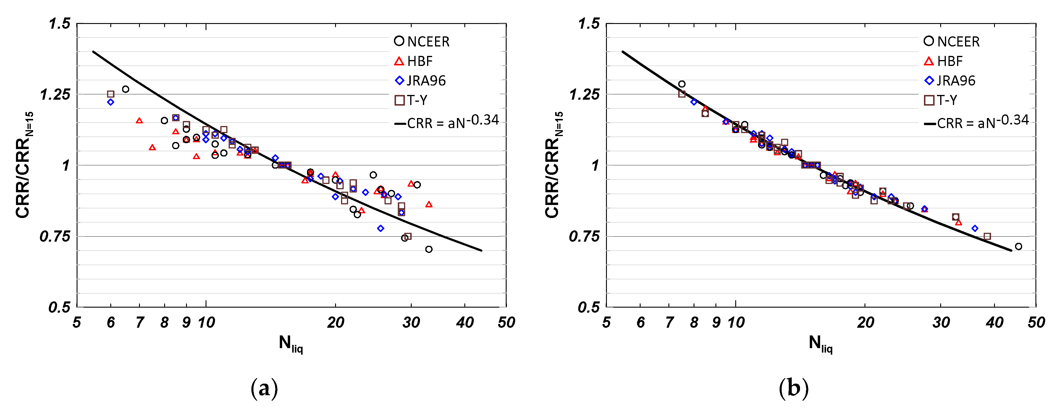
- The relationship between the CRR and the number of uniform loading cycles of the UBCSAND model fit the proposed curves [30] well. The Finn model simulation data deviated from the proposed curves but were still in a reasonable range. Thus, both models were able to adequately model the effects of earthquake magnitude on the CRR.
- (4)
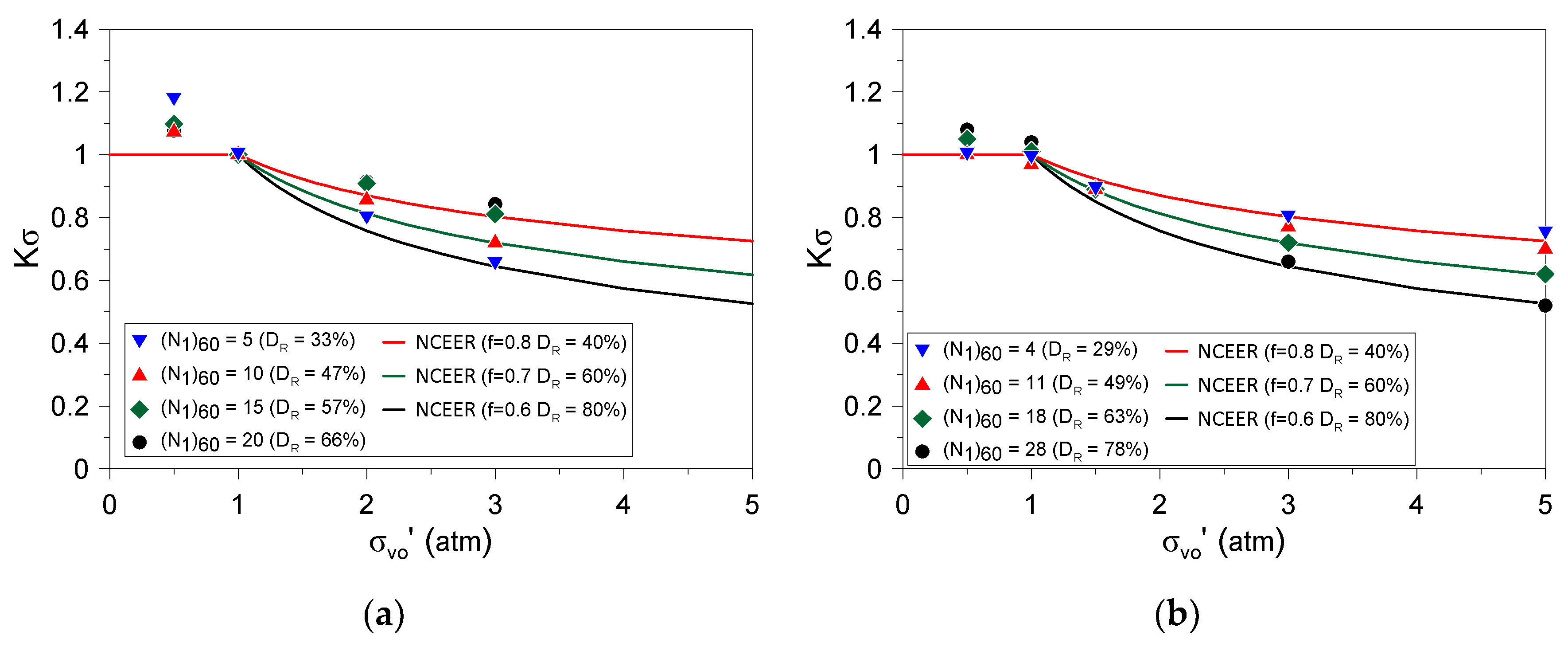
- The UBCSAND model reasonably captured the overburden stress effect and the static shear stress effect on the CRR. Given that the dilatant behavior of sand is not included in the formulations of the Finn model, these effects on the CRR were poorly represented by the Finn model.
- (5)
- The Finn model can be used for the preliminary numerical simulation of structural damage caused by the strength reduction of the liquefiable soil. In general conditions, the UBCSAND model is highly recommended for numerical simulation to obtain reasonable and reliable results.
- (6)
- When the effect of liquefaction hazards or the effectiveness of a mitigation plan need to be evaluated via the numerical analysis, engineers can choose model input parameters according to the (N1)60cs and the simplified liquefaction analysis procedure used in the evaluation of the soil liquefaction occurrence. Then, the numerical analysis can provide reasonable and comparable results.
Author Contributions
Funding
Institutional Review Board Statement
Informed Consent Statement
Data Availability Statement
Acknowledgments
Conflicts of Interest
References
- Giannakou, A.; Travasarou, T.; Ugalde, J.; Chacko, J. Calibration Methodology for Liquefaction Problems Considering Level and Sloping Ground Conditions. In Proceedings of the 5th International Conference on Earthquake Geotechnical Engineering, Santiago, Chile, 11–13 January 2011. Paper No. CMFGI. [Google Scholar]
- Beaty, M.H. Application of UBCSAND to the LEAP centrifuge experiments. Soil Dyn. Earthq. Eng. 2018, 104, 143–153. [Google Scholar] [CrossRef]
- Anthi, M.; Gerolymos, N. A Calibration procedure for sand plasticity modeling in earthquake engineering: Application to TA-GER, UBCSAND and PM4SAND. In Proceedings of the 7th International Conference on Earthquake Geotechnical Engineering, Rome, Italy, 17–20 June 2019; pp. 17–20. [Google Scholar]
- Giannakou, A.; Travasarou, T.; Chacko, J. Numerical Modeling of Liquefaction-Induced Slope Movements. In Proceedings of the GeoCongress 2012: State of the Art and Practice in Geotechnical Engineering, Oakland, CA, USA, 25–29 March 2012; pp. 663–672. [Google Scholar]
- Shriro, M.; Bray, J.D. Calibration of Numerical Model for Liquefaction-Induced Effects on Levees and Embankments. In Proceedings of the 7th International Conference on Case Histories in Geotechnical Engineering, Chicago, IL, USA, 29 April–4 May 2013. [Google Scholar]
- Choobbasti, A.J.; Selatahneh, H.; Petanlar, M.K. Effect of fines on liquefaction resistance of sand. Innov. Infrastruct. Solut. 2020, 5, 1–16. [Google Scholar] [CrossRef]
- Soroush, A.; Koohi, S. Numerical analysis of liquefaction-induced lateral spreading. In Proceedings of the 13th World Conference on Earthquake Engineering, Vancouver, BC, Canada, 1–6 August 2004; p. 2123. [Google Scholar]
- Iraji, A.; Osouli, A. Liquefaction Numerical Analysis of a Cantilevered Retaining Wall Using a Simple Finn-Byrne Model. In Proceedings of the Geo-Congress 2020: Geotechnical Earthquake Engineering and Special Topics, Minneapolis, MN, USA, 25–28 February 2020; pp. 41–50. [Google Scholar]
- Elgamal, A.; Yang, Z.; Parra, E. Computational modeling of cyclic mobility and post-liquefaction site response. Soil Dyn. Earthq. Eng. 2002, 22, 259–271. [Google Scholar] [CrossRef]
- Youd, T.L.; Idriss, I.M.; Andrus, R.D.; Arango, I.; Castro, G.; Christian, J.T.; Dobry, R.; Liam, F.W.D.; Harder, L.F., Jr.; Hynes, M.E.; et al. Liquefaction resistance of soils: Summary report from the 1996 NCEER and 1998 NCEER/NSF workshops on evaluation of liquefaction resistance of soils. J. Geotech. Geoenviron. Eng. ASCE 2011, 127, 817–833. [Google Scholar] [CrossRef] [Green Version]
- Huang, J.H.; Chen, C.H.; Juang, C.H. Calibrating the model uncertainty of the HBF simplified method for assessing liquefaction potential of soils. Sino-Geotech. 2012, 133, 77–86. (In Chinese) [Google Scholar]
- Japan Road Association (JRA). Specification for Highway Bridges, Part. V: Seismic Design; 1996, Substructures. Available online: https://www.pwri.go.jp/eng/ujnr/joint/34/paper/53unjoh (accessed on 4 June 2021).
- Tokimatsu, K.; Yoshimi, Y. Empirical correlation of soil liquefaction based on SPT N-value and fines content. Soils Found. 1983, 23, 56–74. [Google Scholar] [CrossRef] [Green Version]
- Martin, G.R.; Finn, W.L.; Seed, H.B. Fundementals of liquefaction under cyclic loading. J. Geotech. Geoenviron. Eng. 1975, 101, 423–438. [Google Scholar]
- Byrne, P.M. A Cyclic Shear-Volume Coupling and Pore-Pressure Model for Sand. In Proceedings of the Second International Conference on Recent Advances in Geotechnical Earthquake Engineering and Soil Dynamics, St. Louis, MO, USA, 11–15 March 1991; pp. 47–55. [Google Scholar]
- Itasca. FLAC: Fast Lagrangian Analysis of Continua; Itasca Consulting Group Inc.: Minneapolis, MN, USA, 2011. [Google Scholar]
- Puebla, H.; Byrne, P.M.; Phillips, R. Analysis of CANLEX liquefaction embankments: Prototype and centrifuge models. Can. Geotech. J. 1997, 34, 641–657. [Google Scholar] [CrossRef]
- Beaty, M.; Byrne, P.M. An Effective Stress Model for Predicting Liquefaction Behaviour of Sand. Geotech. Earthq. Eng. Soil Dyn. III ASCE 1998, 75, 766–777. [Google Scholar]
- Beaty, M.H.; Byrne, P.M. UBCSAND Constitutive Model. Version 904aR; Itasca UDM: Minneapolis, MN, USA, 2011; p. 69. [Google Scholar]
- Yang, D.; Naesgaard, E.; Byrne, P.M.; Adalier, K.; Abdoun, T. Numerical model verification and calibration of George Massey Tunnel using centrifuge models. Can. Geotech. J. 2004, 41, 921–942. [Google Scholar] [CrossRef] [Green Version]
- Chou, J.C. Centrifuge Modeling of the BART Transbay Tube and Numerical Simulation of Tunnels in Liquefying Ground. Ph.D. Dissertation, University of California, Los Angeles, CA, USA, 2010. [Google Scholar]
- Bray, J.D.; Dashti, S. Liquefaction-induced building movements. Bull. Earthq. Eng. 2014, 12, 1129–1156. [Google Scholar] [CrossRef]
- Ardeshiri-Lajimi, S.; Yazdani, M.; Assadi-Langroudi, A. A Study on the liquefaction risk in seismic design of foundations. Geomech. Eng. 2016, 11, 805–820. [Google Scholar] [CrossRef] [Green Version]
- Chou, J.C.; Lin, D.G. Incorporating ground motion effects into Sasaki and Tamura prediction equations of liquefaction-induced uplift of underground structures. Geomech. Eng. 2020, 22, 25–33. [Google Scholar]
- Seed, H.B.; Idriss, I.M. Soil Moduli and Damping Factors for Dynamic Response Analysis; University of California: Los Angeles, CA, USA, 1970; Rpt. No. UCB/EERC-70/10. [Google Scholar]
- Seed, H.B.; Wong, R.T.; Idriss, I.M.; Tokimatsu, K. Moduli and damping factors for dynamic analyses of cohesionless soils. J. Geotech. Eng. 1986, 112, 1016–1032. [Google Scholar] [CrossRef]
- Hardin, B.O.; Drnevich, V.P. Shear modulus and damping in soils: Measurement and parameter effects (Terzaghi Leture). J. Soil Mech. Found. Div. 1972, 98, 603–624. [Google Scholar] [CrossRef]
- Beaty, M.H.; Perlea, V.G. Several observations on advanced analyses with liquefiable materials. In Proceedings of the 31st Annual USSD Conference and 21st Conference on Century Dam Design-Advances and Adaptations, San Degio, CA, USA, 11–15 April 2011; pp. 1369–1397. [Google Scholar]
- Seed, H.B.; Martin, P.P.; Lysmer, J. Pore-water pressure changes during soil liquefaction. J. Geotech. Geoenviron. Eng. 1976, 102, 323–346. [Google Scholar]
- Idriss, I.M.; Boulanger, R.W. Soil Liquefaction during Earthquakes; Earthquake Engineering Research Institute: Oakland, CA, USA, 2008. [Google Scholar]
- Seed, H.B. Earthquake Resistant Design of Earth Dams. In Proceedings of the Symposium on Seismic Design of Embankments and Caverns, Philadelphia, PA, USA, 6–10 May 1983; pp. 41–64. [Google Scholar]
- Harder, L.F.; Boulanger, R.W. Application of Kσ and Kα correction factors. In Proceedings of the NCEER Workshop on Evaluation of Liquefaction Resistance of Soils, Salt Lake City, Utah, USA, 5–6 January 1996; Youd, T.L., Idriss, I.M., Eds.; Technical Report NCEER-97-0022. National Center for Earthquake Engineering Research: Buffalo, NY, USA, 1997; pp. 167–190. [Google Scholar]


| Parameter 1 | Meaning | Parameter 1 | Meaning |
|---|---|---|---|
| friction | friction angle, φ | ff_c2 2 | C2 of Equation (1) |
| cohesion | cohesion, C | ff_c3 2 | C3, threshold shear strain—the shear strain below which volumetric strain will not be produced |
| dilation | dilation angle, Ψ | ||
| shear | shear modulus, G | ||
| bulk | bulk modulus, B | ||
| ff_c1 2 | C1 of Equation (1) |
| Parameter 1 | Meaning | Parameter 1 | Meaning |
|---|---|---|---|
| m_n160 | (N1)60cs | m_rf | failure ratio, Rf |
| m_kge | elastic shear modulus number, KGe | m_hfac1 2 | accounts for the confining stress effect on the CRR |
| m_ne | elastic shear exponent, ne | ||
| m_kbe | elastic bulk modulus number, KBe | m_hfac2 2 | shear modulus factor to modify the rate of pore pressure generation |
| m_me | elastic bulk exponent, me | ||
| m_kgp | plastic shear modulus number, KGp | m_hfac3 2 | factor to modify post-liquefaction dilation response |
| m_np | plastic shear exponent, np | ||
| m_phif | peak friction angle, φpeak | m_hfac4 2 | factor to control the plastic shear strains after liquefaction and soil dilation |
| m_phicv | constant-volume friction angle, φcv |
| Parameter | Value or Relationship | Parameter | Value or Relationship |
|---|---|---|---|
| KGe | 21.7 × 20 × ((N1)60cs)0.333 | φcv | 33° |
| KBe | 0.7KGe | Rf | 1.1((N1)60cs)−0.15 < 0.99 |
| KGp | KGe × ((N1)60cs)2 × 0.003 + 100 | m_hfac11 | a × (σ′/Pa)b |
| ne/me/np | 0.5/0.5/0.4 | m_hfac2 | 1 |
| φpeak | φcv + 0.1(N1)60cs + max(0, ((N1)60cs − 15)/5) | m_hfac3 | 1 |
| m_hfac4 | 1 |
| Parameter | Value or Relationship | Parameter | Value or Relationship |
|---|---|---|---|
| φ | φcv + 0.1(N1)60cs | C1 | 8.7((N1)60cs)−1.25 |
| C | 1 kPa | C2 | C1 × C2 = C_Finn |
| Tcut | 0 | C3 | 0.005% |
| Ψ | (φ − φcv) | φcv | 33° |
| G (= Gmax) | Equation (11) | hysteretic model | γref = 0.06% |
| B | 1.33G |
| (N1)60cs | NCEER | HBF | JRA96 | T-Y |
|---|---|---|---|---|
| 5 | 0.35 | 0.90 | 0.80 | 0.56 |
| 10 | 0.35 | 0.50 | 0.34 | 0.34 |
| 15 | 0.35 | 0.43 | 0.29 | 0.19 |
| 20 | 0.35 | 0.40 | 0.21 | 0.13 |
| 25 | N.A. | N.A. | 0.11 | 0.10 |
| Procedure | (N1)60cs Range | Relationship 1 |
|---|---|---|
| NCEER | 5~25 | KGp = 0.06X3 + 5.65X2 + 18.18X + 160 |
| HBF | 5~25 | KGp = 0.79X3 − 8.71X2 + 66.85X + 350 |
| JRA96 | 5~30 | KGp = −0.26X3 + 9.02X2 + 6.74X + 280 |
| T-Y | 5~30 | KGp = −0.16X3 + 6.29X2 + 8.00X + 210 |
Publisher’s Note: MDPI stays neutral with regard to jurisdictional claims in published maps and institutional affiliations. |
© 2021 by the authors. Licensee MDPI, Basel, Switzerland. This article is an open access article distributed under the terms and conditions of the Creative Commons Attribution (CC BY) license (https://creativecommons.org/licenses/by/4.0/).
Share and Cite
Chou, J.-C.; Yang, H.-T.; Lin, D.-G. Calibration of Finn Model and UBCSAND Model for Simplified Liquefaction Analysis Procedures. Appl. Sci. 2021, 11, 5283. https://doi.org/10.3390/app11115283
Chou J-C, Yang H-T, Lin D-G. Calibration of Finn Model and UBCSAND Model for Simplified Liquefaction Analysis Procedures. Applied Sciences. 2021; 11(11):5283. https://doi.org/10.3390/app11115283
Chicago/Turabian StyleChou, Jui-Ching, Hsueh-Tusng Yang, and Der-Guey Lin. 2021. "Calibration of Finn Model and UBCSAND Model for Simplified Liquefaction Analysis Procedures" Applied Sciences 11, no. 11: 5283. https://doi.org/10.3390/app11115283
APA StyleChou, J.-C., Yang, H.-T., & Lin, D.-G. (2021). Calibration of Finn Model and UBCSAND Model for Simplified Liquefaction Analysis Procedures. Applied Sciences, 11(11), 5283. https://doi.org/10.3390/app11115283