Micro Vibration Measurement with Microscopic Speckle Interferometry Based on Orthogonal Phase

Abstract

A micro-device vibration measurement method based on microscopic speckle interferometry combined with orthogonal phase is presented. This method utilizes the approximate linear distribution characteristics of orthogonal points (points satisfying the condition that the initial phase difference equal to π/2) to quickly obtain the vibration information of the measured object. Compared with common optical measurement methods, this method does not require scanning imaging and can realize real-time full-field measurement. Moreover, the measurement principle and equipment is simple, so there is no need to introduce a stroboscopic light source or heterodyne device.

1. Introduction

With the increasing requirements for the functionality and miniaturization of electromechanical devices, the application of microelectromechanical systems (MEMS) and nanostructured devices has become more and more important. Vibration of nanometer and micrometer range is one of the most common dynamic characteristics both in the manufacturing process and practical applications of MEMS. By determining its vibration frequency and amplitude through measurement techniques, the non-destructive evaluation and error compensation can be carried out.

Common vibration measurement methods, such as accelerometers, laser displacement meters and digital image correlation (DIC) methods are not suitable for vibration measurement of micro devices. Optical interferometry has the advantages of non-contact, high accuracy, and direct measurement of micro-vibration, so they have been widely used. Common optical interferometry includes homodyne interferometry [1,2,3,4,5,6], heterodyne interferometry [7,8,9,10,11,12], Sagnac interferometry [13] and stroboscopic white light interferometry [14,15,16,17]. Knuuttila, J. V. et al. [3] demonstrated a homodyne scanning Michelson interferometer, which can directly measure the surface acoustic wave in the range of 0.5 MHz to 1 GHz. The sensitivity is about 10⁻⁵ nm/$\sqrt{\mathrm{Hz}}$, and the scanning speed is 49,200 points/h. Fattinger, G. G. et al. [4] used Mach–Zehnder interferometer to measure the vibration of high frequency thin film resonators. The measurement frequency range is 30 kHz to 12 GHz, and the amplitude is less than 10 pm. It also requires scanning to realize the measurement of the whole surface, and it takes 10 h to complete the entire measurement process. Martinussen, H. et al. [7] introduced a modulated heterodyne signal by using two acousto-optic modulators (AOM) in the measurement optical path to measure the vibration of the micro mechanical ultrasonic transducer. The frequency range is from 5 kHz to 35 MHz. The Bessel function method is used for theoretical calculation, so the maximum amplitude that can be measured is far less than the wavelength of the light source. The authors of [8] presented a scanning heterodyne laser interferometer. Under the premise of ensuring high accuracy, the maximum measurement is 300 pm. Kokkonen, K. et al. [15] reported a stroboscopic white light interferometer used to measure the surface acoustic wave generated by a ring-shaped transducer with a working frequency of 74 MHz. The maximum vibration amplitude was 3 nm. We have summarized the frequency and amplitude of the above methods into a table, as shown in

Table 1. The frequency and amplitude of the above methods.

Method	Frequency	Amplitude
Homodyne interferometry	kHz to GHz	pm
Heterodyne interferometry	kHz to GHz	nm
Sagnac interferometry	MHz to GHz	pm
Stroboscopic white light interferometry	MHz	nm

.

At present, optical interferometry has obtained many achievements in the field of high-frequency vibration measurement. However, they generally achieve full-field measurement in a scanning manner, which causes the measurement process to take a long time and cannot achieve real-time measurement.

The electronic speckle pattern interferometry (ESPI) can also be used in the field of non-contact vibration measurement, and can achieve full-field measurement. By analyzing the interferograms, we can obtain the vibration information of the measured object. Researchers have designed the corresponding optical measurement configuration and phase processing algorithm. Bavigadda, V. et al. [18] reported a simple, compact ESPI incorporating holographic optical system for the study of out-of-plane vibration. The time-average subtraction method was used to generate the fringe pattern, and the amplitude and phase image were obtained through path difference modulation. Dai, X. J. et al. [19] proposed a method incorporating amplitude-fluctuation electronic speckle pattern interferometry (AF-ESPI) with radial basis function (RBF) to investigate vibration characteristics of sandwich panels. This method can improve the quality of fringe pattern, but it did not increase the measurement sensitivity. These two methods both require additional signal modulation devices (analog-to-digital converters or signal generators) to modulate the frequency of the reference beam to be consistent with the vibration frequency to achieve the measurement.

In this paper, we propose a new vibration measurement method based on orthogonal phase and microscopic speckle interferometry. The vibration with frequency from 0.5 Hz to 20 Hz is measured and the measurable frequency range can be greatly improved when using a high frame rate camera. The maximum measurable amplitude can reach 60 nm. Compared with the heterodyne method, homodyne method, etc. mentioned above, our method exhibits two main advantages: 1. It can realize real-time full-field measurement without scanning; 2. The calculation process and measurement equipment are very simple, and there is no need to introduce stroboscopic light source or heterodyne device. Additionally, compared with the traditional ESPI technology, our method does not require additional signal modulation devices.

2. Principle

In the optical path of interference measurement, the light intensity signal collected by the charge-coupled diode (CCD) can be expressed as:

$$I=I_1+I_2+2\sqrt{I_1{I}_2}\cos (\theta ),$$

(1)

where I₁ and I₂ are the light intensities of the object beam and the reference beam, respectively, and $\theta$ represents the phase difference between them.

When the measured object vibrates, its trajectory S can be described as:

$$S=A\cos (2\pi f \mathrm{t}),$$

(2)

where A is the vibration amplitude and $f$ is the vibration frequency. These two physical quantities are the physical quantities to be finally measured. At this time, the light intensity signal can be expressed as:

$$\begin{array}{cc}\hfill I& =I_1+I_2+2\sqrt{I_1{I}_2}\cos (\phi +\frac{4\pi S}{\lambda })\hfill \\ & =I_1+I_2+2\sqrt{I_1{I}_2}\cos [\phi +\frac{4\pi A\cos (2\pi f \mathrm{t})}{\lambda }]\hfill \end{array}$$

(3)

where $\phi$ represents the initial phase difference.

When processing light intensity signals with double cosine function in the vibration measurement, the Bessel function method is usually used [20,21,22]. In this method, the amplitude A is required to be far less than the wavelength, which limits the amplitude range of the measurement. By omitting the DC component of the above formula (for they do not contain vibration information) and expanding it according to the Bessel function, we can get:

$$\begin{array}{cc}\hfill I& =2\sqrt{I_1{I}_2}\cos (\phi +\frac{4\pi S}{\lambda })\hfill \\ & =K\cos \phi [J_0(\frac{4\pi A}{\lambda })-2J_2(\frac{4\pi A}{\lambda })\cos 4\pi ft]\hfill \\ & -K\sin \phi [2J_1(\frac{4\pi A}{\lambda })\sin 2\pi ft-2J_3(\frac{4\pi A}{\lambda })\sin 6\pi ft]\hfill \end{array}$$

(4)

where K represents the photoelectric constant before the cosine term, J₀ is the zero-order Bessel function, and J₁, J₂, J₃ correspond to the Bessel function of the corresponding order. It can be seen from Equation (4) that the spectrum of the photocurrent is composed of the fundamental frequency and its harmonics. We use P_n to represent the amplitude of the nth harmonic:

$$P_n=2K{J}_n(\frac{4\pi A}{\lambda })\{\begin{array}{l}\cos \phi \mathrm{when}n\mathrm{is}\mathrm{even}\\ \sin \phi \mathrm{when}n\mathrm{is}\mathrm{odd}\end{array},$$

(5)

In Equation (5), P_n is easy to be measured, but the constants K and $\phi$ are difficult to measure accurately. Therefore, the amplitude A is generally determined by the ratio of two different harmonic amplitudes or the special point (such as maximum value or zero point). This is the principle of the general Bessel function method.

In this paper, the calculation method is more concise. According to the properties of the cosine function, the approximate linear distribution is satisfied near the position of π/2, as shown in Figure 1. (Considering the symmetry of the cosine function, 3π/2 play the same role in (π–2π) as π/2 in (0–π). For simplicity of expression, what we have been discussing in the article is π/2.) When the initial phase difference $\phi$ equal to π/2 and the light intensity, which is determined by the amplitude A, is not too large to exceed the linear region, the vibration trajectory and the light intensity change caused by the vibration are corresponding to each other. We use the orthogonal characteristics to obtain the vibration information from the light intensity signal. The detailed formula derivation will be shown below.

3. Simulation

In order to verify the rationality of the orthogonal characteristics and determine the range of the measurable vibration amplitude, simulations with a series of vibration amplitudes are conducted. In the simulation, when the measured object vibrates, the light intensity of these orthogonal points (the points of $\phi$ equal to π/2) can be expressed as:

$$I=I_1+I_2+2\sqrt{I_1{I}_2}\cos [\frac{\pi }{2}+\frac{4\pi A\cos (2\pi f\mathrm{t})}{\lambda }],$$

(6)

We set $\lambda$ as 532 nm, which is equal to the laser wavelength used in the experiment; $f$ has no effect on the distribution, and it is set to 1 Hz in the simulation. According to Equation (6), in order to satisfy the linear characteristics around π/2, the value of amplitude A should not be too large. We set A as 30 nm, 50 nm, 70 nm, and 90 nm, respectively, for simulation. The real-time position of measured object and the corresponding light intensity curves are shown in Figure 2.

As shown in Figure 2, when the amplitude A is 30 nm and 50 nm, the light intensity curves (Figure 2e,f) are in good agreement with the vibration trajectory (Figure 2a,b). Additionally, when the amplitude A is 70 nm and 90 nm, the light intensity curves (Figure 2g,h) and the vibration trajectory (Figure 2c,d) become no longer consistent. Taking Figure 2h for example, when A is equal to 90 nm, the maximum value of the parameter in the cosine term exceeds the range of (0–π) and frequency doubling phenomenon occurs. At this time, we can get the maximum value I_max and minimum value I_min. Figure 2g also shows frequency doubling phenomenon. As the amplitude of 70nm is not particularly large, the frequency doubling phenomenon is not obvious. It can only be seen that the top and bottom of the light intensity curve become flat. On the basis of simulations and verifications, in order to meet the linear matching range and obtain accurate measurement results, the range of measurable amplitude is within 60 nm.

Additionally, the following relationships can be obtained from Equation (6): when $\frac{4\pi A\cos (2\pi f \mathrm{t})}{\lambda }$ takes the minimum value, the light intensity corresponds to the peak; when the vibration term takes the maximum value, the light intensity corresponds to the valley. The light intensity in these two cases can be expressed as:

$$\begin{array}{l}{I}_{peak}=I_1+I_2+2\sqrt{I_1{I}_2}\cos [\frac{\pi }{2}+\frac{4\pi (-A)}{\lambda }]\\ I_{valley}=I_1+I_2+2\sqrt{I_1{I}_2}\cos [\frac{\pi }{2}+\frac{4\pi (A)}{\lambda }]\end{array}$$

(7)

Compared with the Equation (4), which uses Bessel function, the expression is greatly simplified and no longer contains the double cosine function. As long as we get I₁, I₂ and the corresponding peak value of light intensity I_peak (or I_valley), we can get the amplitude A.

Then, we conduct the second simulation to analyze the influence of $\phi$ with a certain offset which is not equal to π/2. In this case, the light intensity can be expressed as:

$$I=I_1+I_2+2\sqrt{I_1{I}_2}\cos [\frac{\pi }{2}+\sigma +\frac{4\pi A\cos (2\pi f \mathrm{t})}{\lambda }],$$

(8)

We take A to be 40 nm in the measurable range, $f$ is still 1 Hz, and $\sigma$ represents the magnitude of the offset. The real-time position of the measured object and the light intensity curves under different offset are shown in Figure 3:

From Figure 3b–h, the absolute value of $\sigma$ is reduced from 3π/10 to 0, and then increased from 0 to 3π/10. With the increase in the absolute value of $\sigma$, the initial value in the cosine term gradually deviates from π/2, then the light intensity curves and the vibration trajectory no longer match. When the absolute value of $\sigma$ is too large, the light intensity signal will appear frequency doubling, as shown in Figure 3b,h. At this time, the maximum value I_max will appear at the upper limit of the light intensity (Figure 3b), or minimum value I_min will appear at the lower limit (Figure 3h). When $\sigma$ equal to 0, the light intensity curves will be symmetrically distributed with respect to (I_max + I_min)/2, as shown in Figure 3e.

Through the above simulation, we can summarize the corresponding relationship between the vibration trajectory and the light intensity curves. When the amplitude A meets the reasonable range selected and $\sigma$ equal to 0, the light intensity curves will be symmetrically distributed with respect to (I_max + I_min)/2, as shown in Figure 3e. According to the characteristic that the light intensity curve is symmetrically distributed about the symmetry axis I = (I_max + I_min)/2, we can obtain these points that satisfy the orthogonal characteristic.

From the light intensity curves of these points, the vibration frequency $f$ can be obtained directly. To obtain the vibration amplitude, we can first artificially increase the A or $\sigma$ to get the I_max and I_min. By substituting them into Equation (8), when the cos term is +1, it corresponds to the I_max, and when the cos term is −1, it corresponds to the I_min, so the initial light intensity I₁ and I₂ can be obtained, respectively. Then, we return to the light intensity curve that satisfies the orthogonal characteristics to obtain I_peak (or I_valley), as in Figure 3e; the vibration amplitude can be obtained by Equation (7). The specific derivation process is detailed in Section 4.1.

4. Experiment

The schematic diagram of the microscopic speckle interference vibration measurement system is shown in Figure 4. The light source is a single longitudinal mode laser with a wavelength of 532 nm, and the output power is 100 mW. The CCD we use is $640\times 480$ spatial resolution at low frame rate and $160\times 120$ spatial resolution at the highest frame rate of 400 frames/s. The exposure time of the CCD is 300 microseconds. The pixel size of the CCD is 4.8 um × 4.8 um. The objective lens numerical aperture is 0.25 and the magnification is 10. The vibration signal of the measured object is introduced by the displacement platform produced by German PI company, and the accuracy of the vibration signal is higher than 0.1 nm.

During measurement, the laser beam is split into measuring beam and reference beam by beam splitter. The measuring beam is focused on the measured object through the microscope objective and then reflected back to the beam splitter. Similarly, the reference beam is reflected by the reference object. The two beams will interfere after passing through the beam splitter, and then are detected by the CCD. In order to ensure the continuity of the light intensity curve, we need to ensure that there are at least 20 collection points for each vibration period. Therefore, the upper limit of the vibration frequency can be measured is 20 Hz corresponding to 400 frames/s. The measured frequency range depends on the camera acquisition frequency. If a camera with a high-speed acquisition frame rate is used, the measurement frequency range can be further expanded. The optical path structure diagram is shown in Figure 5.

4.1. Speckle Interference Experiment

The measured object used in the experiment is the model 3325 silicon wheat produced by Goertek company, with the size being $3\times 2\times 1.2$ mm³ ($L\times W\times H$). After the light beam passes through the microscope objective lens, a circular spot with a diameter of 1.5 mm will be generated on its surface, as shown in Figure 6.

The speckle interference generated by the rough surface has the characteristics of random distribution, so the initial phase difference $\phi$ is randomly distributed in the range of (0-π). We need to find out the points that satisfies $\phi$ equal to π/2. In our experiments, we found that when a $6\times 6$ pixel window is used to search, we can get at least one pixel that satisfies the orthogonal condition among these 36 pixels. Combining the random distribution characteristics of speckle interference and cosine curve profile for analysis, it is reasonable to exist more than one pixel at the position of $\phi$ equal to π/2 or very close to π/2 in 36 pixels. Using the algorithm we have written in MATLAB, the light intensity curves of 36 points can be obtained. According to the distribution characteristics described above, the points that satisfy the orthogonal characteristic can be found out. If we cannot find any point that meets the condition, we need to further expand the search area.

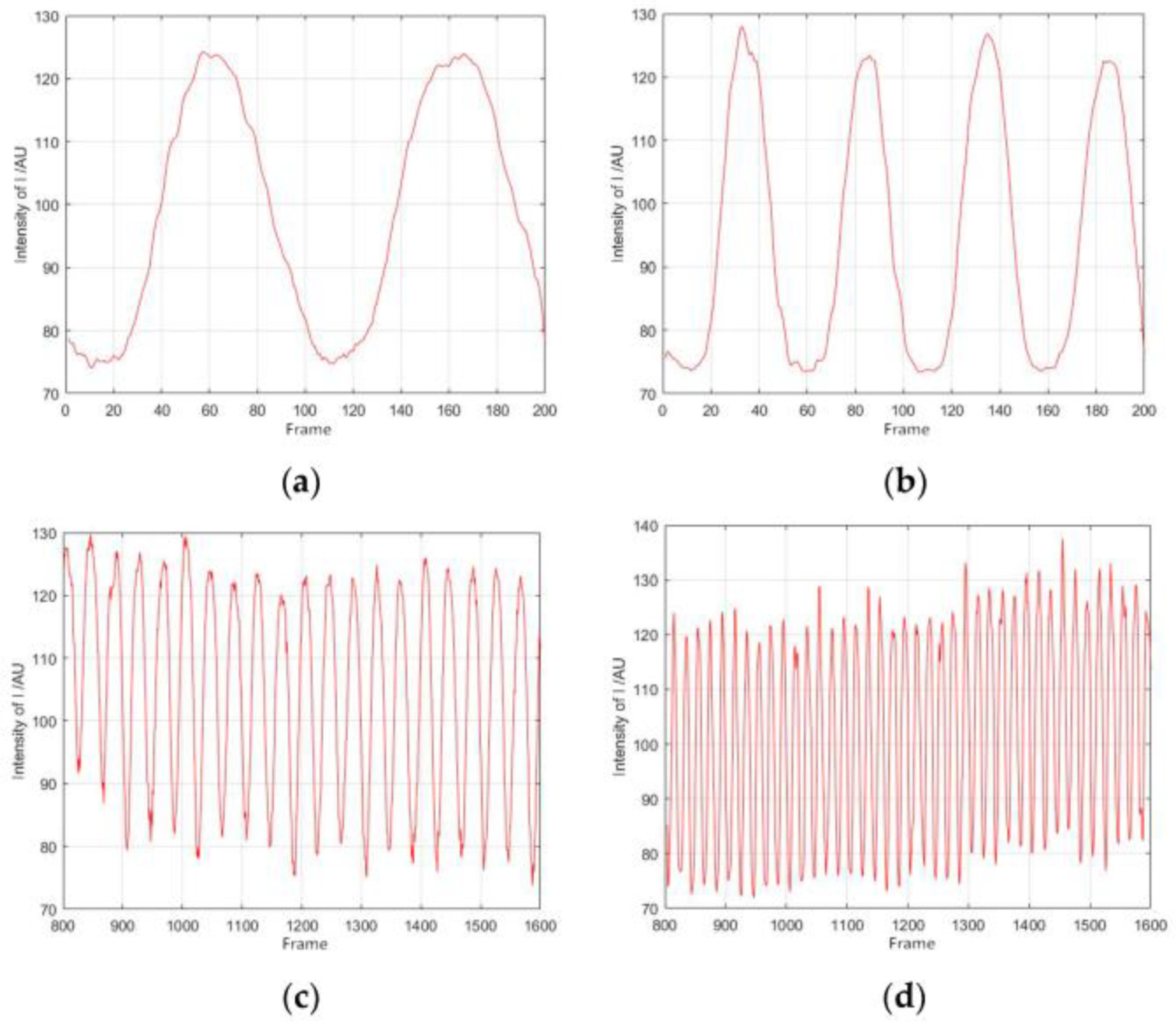
In order to make full use of the spatial resolution of the CCD, we flexibly choose different acquisition frame rates for different measured frequencies. Figure 7 shows images collected by the CCD at 50 frames/s. Figure 8 shows the light intensity curves obtained under the condition with the same amplitude (40 nm in the article) and different frequencies. The vibration frequencies of (a) and (b) are 0.5 Hz and 1 Hz, respectively. The acquisition frame rate of CCD is set to 50 frames/s, and the 200 frames shown in the figures correspond to 4 s. The vibration frequencies of (c) and (d) are 10 Hz and 20 Hz, respectively. At this time, the acquisition frame rate of CCD is set to 400 frames/s. In order to make the light intensity curves not too dense, we show the light intensity curves of 800 frames in 2 s.

Then, we measure the vibrations with the same vibration frequency (10 Hz selected in the article) and different amplitudes, as shown in Figure 9. For the same reason mentioned above, we choose the light intensity curves of 800 frames in 2 s.

In order to obtain the vibration amplitude, we need to calculate the values of I₁, I₂ and the peak value I_peak. When frequency doubling phenomenon occurs, the maximum value I_max or minimum value I_min can be obtained. When the amplitude is too large, as shown in Figure 9d, we can read I_max and I_min simultaneously in one image. More commonly, I_max and I_min are read out, respectively, as shown in Figure 3b,h. Taking Figure 9d as an example, the average values of I_max and I_min are 160 and 12, and (I_max + I_min)/2 is 86. By substituting them into Equation (8), we can get:

$$I_1+I_2+2\sqrt{I_1{I}_2}\cos [0]=160,$$

(9)

$$I_1+I_2-2\sqrt{I_1{I}_2}\cos [0]=12,$$

(10)

We can get I₁ = 64.91 and I₂ = 21.09. With the values of I₁ and I₂, the vibration amplitude can be obtained by Equation (7). Taking Figure 9b as an example, the average value of the 20 peaks is 136, so we take I_peak equal to 136:

$$I_1+I_2+2\sqrt{I_1{I}_2}\cos [\frac{\pi }{2}+\frac{4\pi (-A)}{\lambda }]=136,$$

(11)

By calculation, A is 31.4 nm. The amplitude of Figure 9b is 30 nm, and the relative error is 4.6%.

To get the accurate amplitude, we need to know the accurate periodic peak value I_peak. As we mentioned in the above experimental part, due to the limitation of the CCD collection frequency, 20 points are collected per vibration period. There is no complete correspondence between the measured vibration period light intensity and the actual vibration period light intensity. Therefore, there is a certain difference between the I_peak we obtained and the actual I_peak, which is the main reason for the error. By using a high-frequency camera, the error can be reduced by increasing the number of points collected per vibration period.

For vibration trajectory and the light intensity change are corresponding to each other, the vibration frequency can be directly obtained: f = 10 Hz. Finally, we can obtain the vibration frequency and amplitude of the measured object.

4.2. Realization of Surface Measurement

We have completed the measurement of vibration of speckle interference. Then, we will show how to use our method to realize surface measurement.

The key of this method is to find the pixels that satisfy the orthogonal characteristics. We choose the speckle pattern when the amplitude is 40 nm and the frequency is 10 Hz. It can be seen that the interference imaging area is approximately a circle. The resolution of the image is $160\times 120$ pixels. We select the $120\times 120$ pixels area for calculation, and the starting pixel is (1, 21). Then, the selected area is traversed with a $6\times 6$ pixel window, and $20\times 20$ windows can be obtained, as shown in Figure 10a. It can be seen from Figure 10a that the four corners of the red square dotted frame are black and do not contain vibration information, so the windows at these positions need to be excluded. Then, we need to find one point that satisfies the orthogonal characteristics in each of the remaining windows. After calculating the vibration amplitude of these points, the surface distribution can be obtained by connecting these points and smoothing. In the end, we get an approximately circular surface distribution, as shown in Figure 10d. Among these points, the maximum amplitude obtained is 41.8 nm, the minimum amplitude is 38.7 nm, the average value is 40.3 nm, and the standard deviation is 0.28.

5. Conclusions

We propose a micro-device vibration measurement method based on microscopic speckle interferometry combined with orthogonal characteristics. We have measured vibrations with frequency from 0.5 Hz to 20 Hz used the experimental device, and the maximum amplitude that can be measured is 60 nm. Our measurement method has two advantages: 1. It does not require scanning for imaging, so it can directly achieve real-time full-field measurement; 2. The measurement principle and equipment is simple, so there is no need to introduce a stroboscopic light source, heterodyne device or additional signal modulation devices.

This method enriches the measurement range of optical vibration measurement technology to a certain extent. The main reason for limiting the upper limit of the measurable vibration frequency is the acquisition frequency of the camera. For example, the acquisition frequency of Mini-AX200 camera produced by Photron Company can reach 160,000 frames/s, which is 400 times that of our camera. In theory, the upper limit of the vibration frequency that can be measured with this camera can reach 8 kHz. This theoretical derivation needs to be verified by further experiments.