Knee Osteoarthritis Classification Using 3D CNN and MRI

Abstract

Osteoarthritis (OA) is the most common form of arthritis and can often occur in the knee. While convolutional neural networks (CNNs) have been widely used to study medical images, the application of a 3-dimensional (3D) CNN in knee OA diagnosis is limited. This study utilizes a 3D CNN model to analyze sequences of knee magnetic resonance (MR) images to perform knee OA classification. An advantage of using 3D CNNs is the ability to analyze the whole sequence of 3D MR images as a single unit as opposed to a traditional 2D CNN, which examines one image at a time. Therefore, 3D features could be extracted from adjacent slices, which may not be detectable from a single 2D image. The input data for each knee were a sequence of double-echo steady-state (DESS) MR images, and each knee was labeled by the Kellgren and Lawrence (KL) grade of severity at levels 0–4. In addition to the 5-category KL grade classification, we further examined a 2-category classification that distinguishes non-OA (KL ≤ 1) from OA (KL ≥ 2) knees. Clinically, diagnosing a patient with knee OA is the ultimate goal of assigning a KL grade. On a dataset with 1100 knees, the 3D CNN model that classifies knees with and without OA achieved an accuracy of 86.5% on the validation set and 83.0% on the testing set. We further conducted a comparative study between MRI and X-ray. Compared with a CNN model using X-ray images trained from the same group of patients, the proposed 3D model with MR images achieved higher accuracy in both the 5-category classification (54.0% vs. 50.0%) and the 2-category classification (83.0% vs. 77.0%). The result indicates that MRI, with the application of a 3D CNN model, has greater potential to improve diagnosis accuracy for knee OA clinically than the currently used X-ray methods.

1. Introduction

The most common form of joint disorder in the United States is osteoarthritis (OA) [1]. Knee OA can cause pain and is the number one disease at causing loss of ability to perform daily activities such as walking and stair climbing [2]. Knee OA is associated with age [3] and is characterized by the loss of articular cartilage volume [4]. OA is viewed as a “whole-organ” disorder, manifesting damage to a range of articular structures, especially the hyaline cartilage, meniscus, periarticular bone, ligaments, and tendons [5]. Despite its importance for public health, we have no interventions that effectively modify the OA disease process [6]. The absence of useful biomarkers to detect OA progression is a major technological obstacle to the development of treatment and prevention of knee OA [7].

While joint replacement is effective for treating end-stage OA, the evaluation of potential disease-modifying treatments in populations meeting current clinical criteria for OA has had limited success [6]. In the past decade, early diagnosis and early treatment strategies in rheumatoid arthritis have reduced patient morbidity and associated costs [8]. The early diagnosis and treatment of OA conditions may similarly improve outcomes and reduce disability and costs for OA. However, the absence of useful image biomarkers to detect OA progression has been a critical technology gap in the early diagnosis and treatment of OA [9].

The conventional radiographs (X-rays) are commonly used for routine knee OA examinations. An X-ray of a joint with osteoarthritis typically shows a narrowing of the space between the bones of the knee joint where the cartilage has worn away. However, symptoms of knee OA may arise before the damage can be seen in standard X-rays. For example, Roemer et al. [10] described how X-rays are unable to show certain structural phenotypes of OA and cannot detect some detrimental findings which can indicate risk of disease that would progress rapidly.

The advent of magnetic resonance imaging (MRI) offers the promise of addressing the critical technology gap by allowing quantification of structural damage in joints. For this reason, radiologists at hospitals often use the more sensitive magnetic resonance imaging (MRI) for OA early detection. Juras et al. [11] pointed out that OA needs early detection, and MRI is a noninvasive way for detecting early biomarkers. To promote the evaluation of OA MRI biomarkers, the National Institutes of Health (NIH) launched the Osteoarthritis Initiative (OAI) cohort study, which includes four clinical centers that recruited approximately 4800 men and women (ages 45–79 years) with or at risk for knee OA. The OAI collected a wealth of data on its participants over an eight-year span. The study included annual knee MRIs for the first four years and then biannual knee MRIs for the subsequent 4 years [12]. One of the goals of creating the OAI dataset was to discover the objective, measurable standards of disease diagnosis and progression, and to determine the predictive role of MRI changes for subsequent radiographic and clinical changes related to the development of knee OA.

The 3-dimensional (3D) MR images allow for both viewing the knee as a “whole organ” and depicting all of the tissues of the joint [13]. While cartilage degradation and other biomarkers can be manually detected, it is time-consuming to process the volume of 3D MR images. Thus, there is a need to automate these processes with machine learning techniques.

Convolutional neural networks (CNNs) are a class of deep learning techniques that are designed to work with images and can remove the need for handcrafted feature extractors [14]. CNNs have been used for various image classification tasks, with recent studies developing CNN models for medical image analysis. The early work of using CNNs to classify knee OA was mainly applied to radiographic (X-ray) images [15,16,17,18].

Anthony et al. employed the classical VGG-16 CNN architecture and transferred learning with X-ray images to determine the OA severity level [15]. These images were preprocessed using an SVM and Sobel edge detector in order to locate the knee joint area. Their study used X-ray images from the OAI. A set of 4446 X-rays were used in this study, representing a total of 8892 knees. When classifying the five Kellgren and Lawrence (KL) grades, they achieved an accuracy of 59.6%. Later, in another work, the same group updated the preprocessing step to use a fully convolutional neural network (FCN) to determine the bounding box of the knee joint. The FCN method was found to be highly accurate in determining regions of interest (ROI), and when combined with a CNN for classification, the method achieved an accuracy of 61.9% [16].

Unlike the two-stage frameworks developed in [15,16], a recent work [17] proposed an end-to-end CNN architecture for knee OA severity assessment without using a neural network for preprocessing. This method used branches in its CNN that are referred to as “attention modules”, which provide an unsupervised determination of the ROI of X-ray images. Another recent work added a long short-term memory (LSTM) classifying step following the CNN layers in their network [18]. Given the nature of LSTM for processing sequential data, additional images were generated in a preprocessing step by cropping a fixed ROI and rotating the cropped image by 5, 10, −5, and −10 degrees. The original image and augmented images were stacked, giving about 4600 images used for training and about 480 for testing. Their work also used images from the OAI and achieved an accuracy of 75.28% for the 5-category classification.

It can be seen that 3D CNNs have developed quickly and are attracting interest as a method for analyzing sequences of images or other volumetric data. In a recent study, a 3D CNN was used for classifying real-world objects [19]. Depth information was used to create a 3D shape that was converted into a volumetric representation (voxels) to be classified by the 3D CNN. In addition, 3D CNNs have shown to be useful in medical image processing. When classifying lung nodules, working with 3D volumetric data in a 3D CNN outperformed 2D CNNs [20]. Wang et al. applied a 3D CNN model to calculate the probability of needing a total knee replacement (TKR) within the next nine years [21]. Their work demonstrated that the automated discovery of OA biomarkers from turbo spin echo (TSE) and double-echo steady-state (DESS) images could outperform models that use only demographic and clinical data. Another work explored this area using the popular 2D U-Net architecture for the segmentation of cartilage and meniscus in the knee, which were fed into a 3D CNN for classifying the severity of the cartilage and meniscus lesions [22]. Given the large amount of volumetric data, another recent work for classifying knee lesions used cropping of 3 ROIs from knee MRI to reduce the dimensionality before processing by multiple 3D CNN [23]. Aside from these applications, 3D CNNs have also been applied to segmentation problems including knee cartilage segmentation [24] and segmentation of brain lesions [25].

For knee OA severity classification, while previous methods used 2D CNNs to analyze X-ray images, in this work we propose a method using a 3D CNN and MR images. The details of the proposed method is introduced in the next section.

2. Materials and Methods

2.1. Method Overview

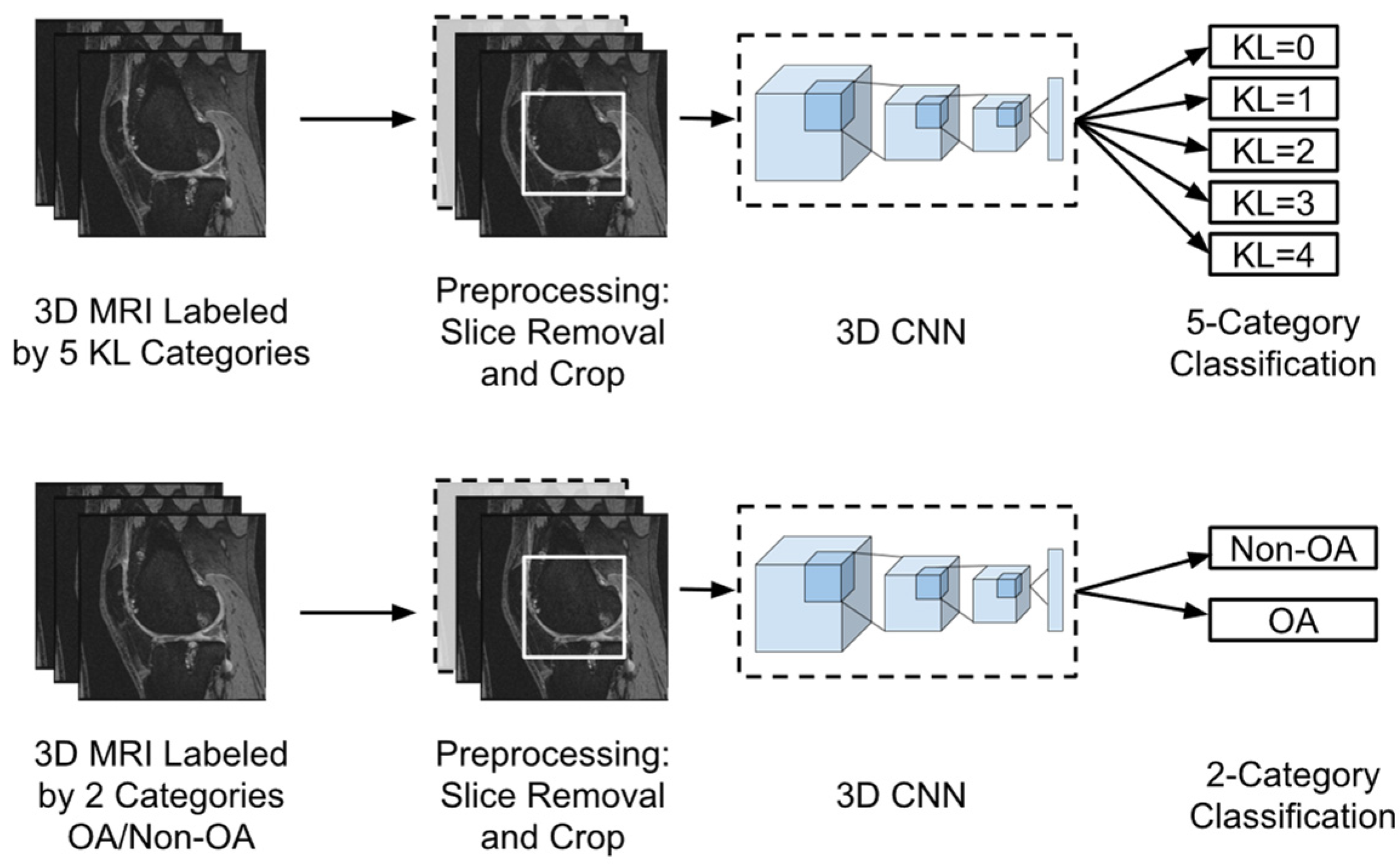
Knee MR imaging produces a 3D representation of the knee joint, utilizing a sequence of 2D images taken laterally across the knee. Given the 3D nature of MR images, 3D CNN can be advantageous in evaluating the whole sequence of images as one unit. Through the implementation of 3D kernels, information from adjacent slices could be integrated. Therefore, 3D features that may not be detectable using 2D CNN could be potentially captured.

For this study, we built a machine-learning model capable of analyzing sequences of MR images for each knee as input, with output given as one of the five KL grades. We further trained another model by relabeling the samples into OA and non-OA categories according to the clinical standard, i.e., patients with KL ≤ 1 are diagnosed as non-OA cases while patients with KL ≥ 2 are considered as OA. An overview of the proposed models is described in Figure 1.

In addition to MRI, we also studied traditional X-ray images, with an interest of finding out which imaging modality coupled with the modern CNNs can achieve better accuracy for knee OA diagnosis. We employed several state-of-the-art 2D CNN models, including VGG 16, ResNet50, DenseNet, etc. These models were trained to classify X-ray images into five KL categories. The one with the best accuracy was selected and further applied for the binary OA/non-OA classification. The pipelines for X-ray images are similar to those illustrated in Figure 1, except the 3D CNN is replaced by a 2D CNN and the preprocessing step for X-ray is to cut each pair of knees into individual ones. The X-ray images and MR images were obtained from the same group of patients, and the separation of training, validation, and testing sets were kept the same at the patient level for all the models trained and compared in this work.

2.2. Dataset

The dataset used in this study was from the public database Osteoarthritis Initiative (OAI). Most of the patient samples in the OAI dataset include an X-ray image; however, many do not have an accompanying MRI sequence. For this study, we used a subset of the OAI data with 1100 knees, with each knee having both MRI and X-ray available. The 3D DESS MRI data for each knee contain a sequence of 160 2D images, while there is one X-ray image containing both knees from a patient. The dataset was selected with an equal distribution among different OA severity levels (0–4) measured by the Kellgren and Lawrence (KL) grades.

A common practice in machine learning is to split the available dataset into three subsets known as the training set, validation set, and testing set [26]. Machine learning models learn from the training set with the validation set being used during the training process to tune parameters [27]. The testing set is not seen during the training process but rather is held back until the end of the study. The available dataset was randomized and then split into groups balanced by the KL grade with 800 training samples, 200 validation samples, and 100 testing samples. Each set contains a balanced number of samples from each of the five KL categories.

Table 1. Distribution of 5 KL grade categories into training, validation, and testing sets.

Set	KL = 0	KL = 1	KL = 2	KL = 3	KL = 4	Total
Training	160	160	160	160	160	800
Validation	40	40	40	40	40	200
Testing	20	20	20	20	20	100
Total	220	220	220	220	220	1100

shows the distribution of the data.

2.3. Preprocessing: Subregion Selection

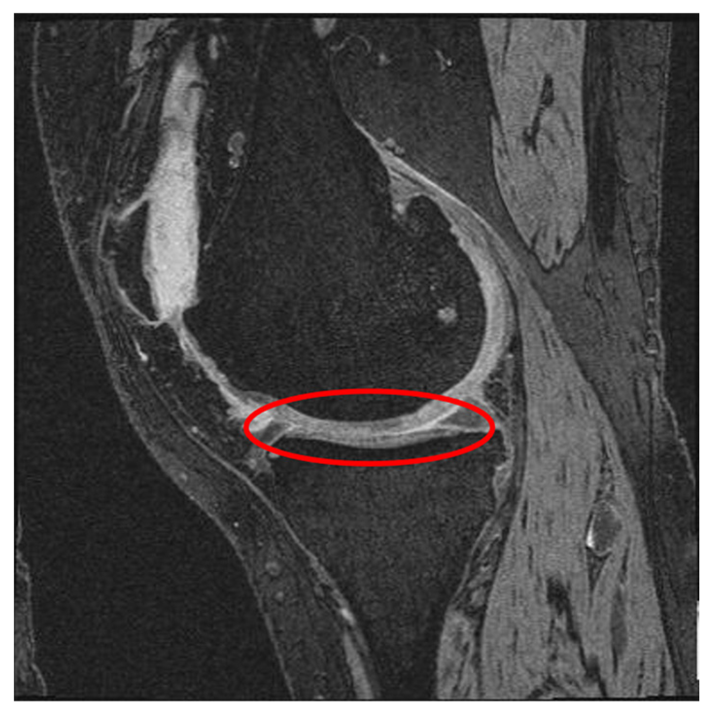
Unlike natural images where useful information could appear anywhere, in medical images, features are usually located in fixed locations. As an example, the knee MR image shown in Figure 2 contains large bone areas and many other tissues. The important indicators for knee OA are often observed near the cartilage and joint region of femur and tibia bones. Therefore, we can reduce the input dimensionality by cropping a subregion of the images.

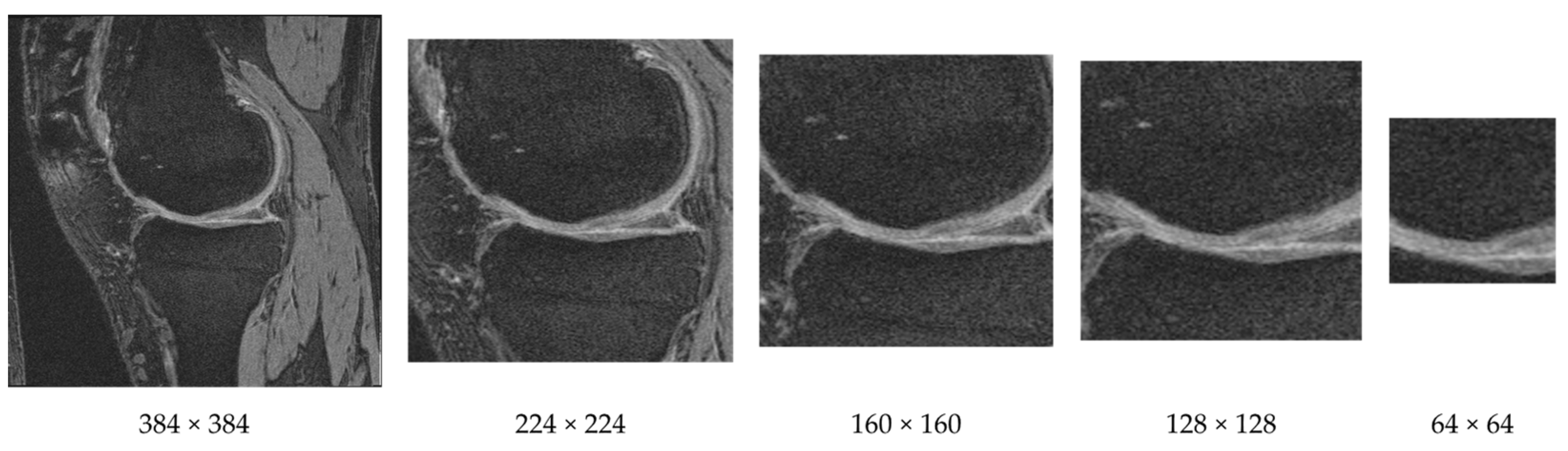
We cropped each image as a preprocessing step that helps to keep the cartilage region while removing regions that are less informative for knee OA classification. We cropped the image (original size 384 × 384) from the center using both square and rectangular regions. An example of cropping a knee MR image to various sizes is provided in Figure 3. Through various tests we discovered that the window size of 160 × 160 achieved the highest F-measure.

2.4. Preprocessing: Slice Removal

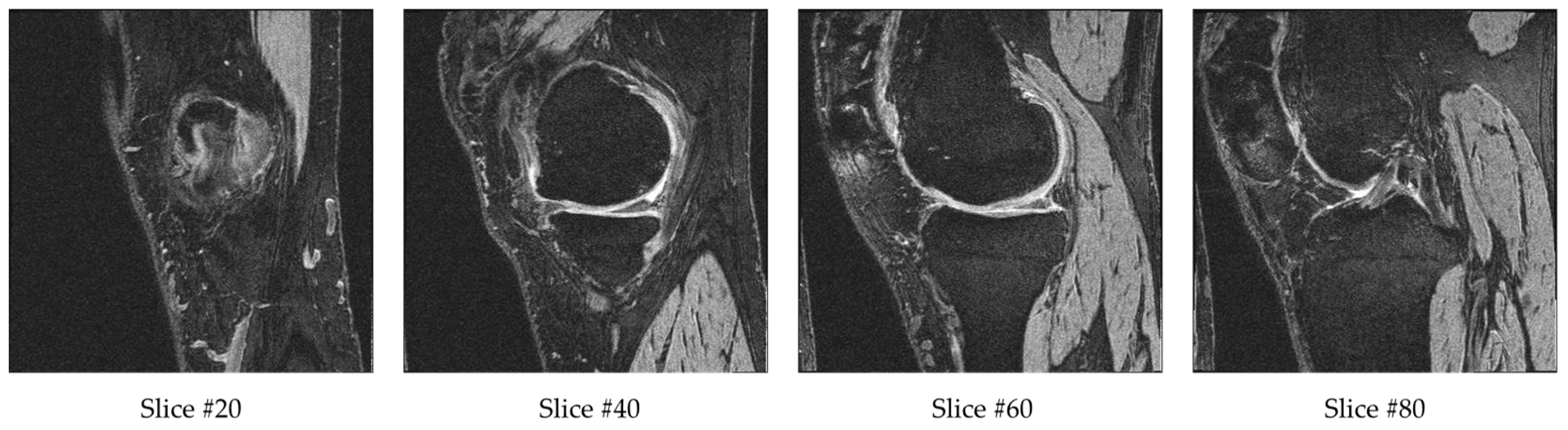
Each sample in the database contains a sequence of 160 MR images. After cropping, the input dimensions of 160 × 160 × 160 were still very high. To further reduce the input data dimensionality, we removed some of the outer and center slices. The reason for removing a few beginning and ending slices is that they do not contain bone or cartilage information. Therefore, they are not likely to contain information related to OA. The reason for removing the middle range slices is that they have ill-defined cartilage regions and blurry bone boundaries due to the transition of medial and lateral bone happening in this range. Example slices are provided in Figure 4. Slice #20 has a small bone region starting, while slice #40 and #60 have larger bones with clearly defined bone boundaries and cartilage. Slice #80 is in the transition range, and therefore the cartilage and bone boundaries are unclear. For each sequence, we excluded the first 10 slices (1–10), middle 20 slices (71–90) and final 10 slices (151–160). The remaining 120 slices (11–70, 91–150) from the 160 slices were fed into the 3D CNN model. This is about 13% of the original 384 × 384 × 160 volume.

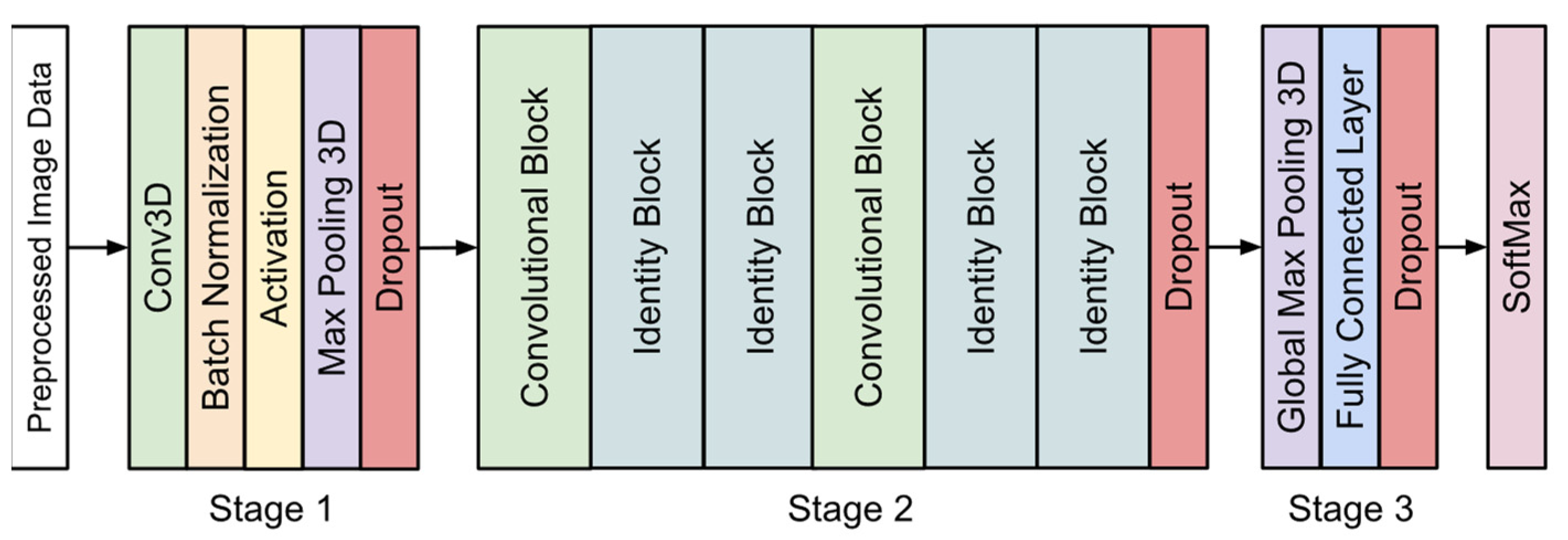
2.5. 3D CNN Model for MRI

The architecture of the 3D CNN model proposed in this study is shown in Figure 5. The structure was inspired by the work performed by Wang et al. [21]. The most important difference between 3D CNNs and 2D CNNs is that 3D CNNs use 3D convolutional kernels to process a volumetric patch of a scan, while 2D CNNs process a single anatomical plane. The 3D convolutional kernels incorporate information from adjacent slices and are therefore able to extract 3D features, which are not detectable from 2D CNNs. As shown in Figure 5, three stages are included in the proposed 3D CNN model before the final softmax layer. The details of the model are discussed below.

Stage 1 of the model began with a convolutional layer containing 32 kernels of size 7 × 7 × 7 with a stride of 2 × 2 × 2. This was followed by batch normalization and an activation layer using the ReLU function. A max-pooling layer was added with a window size of 2 × 2 × 2 and a stride of 2 × 2 × 2. Finally, a dropout layer was placed before the start of the residual blocks. We used dropout layers in each stage of our 3D CNN model to help reduce overfitting. Each dropout layer used a rate of 0.5, which gives each node a 50% chance of being set to 0.

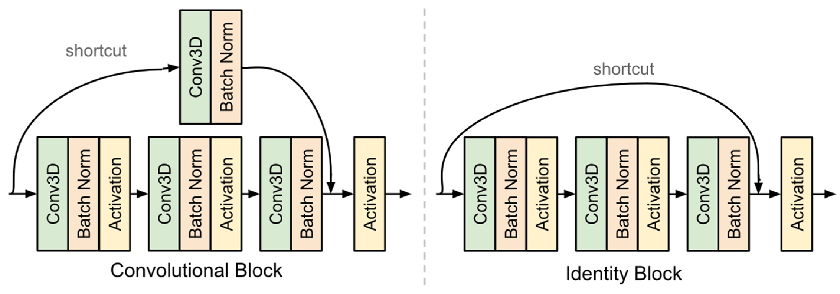
The second stage of the model contained a sequence of six residual blocks [28]. Each residual block featured a shortcut connection from the input to the output. There were two types of blocks used in this model as shown in Figure 6. The convolutional block features a convolutional layer in the shortcut path. This layer was used when the input dimensions were changed. The identity block did not have any layers in the shortcut path and was used when the input and output dimensions matched. This stage also ended with a dropout layer.

The final stage of the model used global max pooling, followed by a fully connected layer of size 1024 and a dropout layer. The last layer of the model uses the softmax function, which outputs the possibilities of the sample belonging to each category.

The model was implemented in Python using the Keras library with TensorFlow as a backend. The model was trained using a batch size of 15 with early stopping based on validation loss. The Adam optimization function was used with a learning rate 0.001. The training was performed on a high-performance computer with a NVIDIA Tesla V100 32 G GPU.

2.6. Classic 2D CNN Architectures for X-ray

When building our dataset, we selected patients which had an MRI volume as well as an X-ray image of the same knees. To develop the model for X-ray, we employed a variety of state-of-the-art 2D CNN architectures. VGG16 [29] was one of the earlier deep learning models, and it showed superior performance in many applications. ResNet50 [28] used the concept of residual blocks in which a shortcut connection is added after a series of layers. Our proposed 3D model utilizes a 3D variation of the ResNet50 convolutional and residual blocks as well. Inception-v3 [30] is the representation of the deep learning networks with inception modules and one of the first models to make use of batch normalization. Inception-ResNet [31] is a hybrid of Inception-v3 with residual connections. DenseNet [32] implements dense blocks in which convolutional layers of the same size are connected to every other layer in front of them.

While an MRI volume contains just one knee, an X-ray image contains both. These X-ray images were split in half, and all the left knees were flipped so the right and left knees are aligned. The pretrained ImageNet weights were used for transfer learning. The last softmax layer was retrained using the X-ray data while the previous layers were not changed. Input images were scaled to a size of 224 × 224 or 299 × 299, depending on the architectures of different models. Since the pretrained networks were trained with RGB images, we duplicated each gray level X-ray image three times to feed it into the three input channels.

3. Results

3.1. 3D CNN Using MRI Data

Table 2. Confusion matrix for the 5-category KL classification by the 3D CNN model on the validation set. A0 denotes samples that are actually with KL = 0 and P0 denotes samples that are predicted as KL = 0 by the model.

Act.\Pred.	P0	P1	P2	P3	P4	Total	Acc.
A0	28	7	5	0	0	40	70.0%
A1	15	18	2	5	0	40	45.0%
A2	7	10	15	7	1	40	37.5%
A3	0	2	2	24	12	40	60.0%
A4	0	0	0	4	36	40	90.0%
Total	50	37	24	40	49	200	60.5%

shows the performance of our 3D CNN model in a confusion matrix of actual vs. predicted level for the 5-category classification. It should be noted that results presented in this subsection and the following two subsections are based on the validation set. The testing set was used once as a final evaluation step in Section 3.4 only. Observing the results in Table 2, we found that the two boundary categories, i.e., KL = 0 and KL = 4, are relatively easier to classify with a high accuracy of 70% and 90%, respectively. The middle categories are more difficult to classify. For category KL = 1, the accuracy is only 45%. However, most misclassified cases (15 out of 22 misclassified ones) were for KL = 0, which is less severe than those misclassified into higher KL grades, since clinically, both KL = 0 and KL = 1 are considered as non-OA. Category KL = 2 had the lowest accuracy 37.5%, and most of these misclassified cases went to KL = 0 and KL = 1. It is worth further examining why this category was considered more similar to non-OA class by the model when clinically this category is considered as an OA class.

Using the same 3D CNN architecture, we trained another model with the input da-ta labeled as non-OA (KL ≤ 1) and OA (KL ≥ 2).

Table 3. Confusion matrix for the 2-category OA/non-OA classification by the 3D CNN model on the validation set.

Act.\Pred.	Non-OA	OA	Total	Acc.
Non-OA	71	9	80	88.8%
OA	18	102	120	85.0%
Total	89	111	200	86.5%

shows the confusion matrix of the 2-category model.

3.2. Ablation Study

The accuracy of our 3D CNN model is based on the preprocessing steps as well as the architecture.

Table 4. Effects on accuracy for preprocessing steps and architecture of the 3D CNN model.

Crop	Slice Removal	Dropout	Res Layers	Acc
√	√	√	√	86.5%
X	√	√	√	81.5%
√	X	√	√	82.0%
√	√	X	√	80.0%
√	√	√	X	73.0%

Note: “√” indicates the feature is included; “X” indicates the feature was removed.

demonstrates the effects of removing individual aspects of our model. The first row shows the accuracy of the model with all strategies used. While our final model used a cropped size of 160 × 160, for this ablation study we used a larger size of 224 × 224, which was the largest that could be used—given memory constraints—to generate the performance without cropping (second row in Table 4). It is worth noting that when we provided more information (larger crop), the accuracy dropped by 5%. To test the effect of slice removal, we removed the slice selection step and used all 160 slices. Similar to cropping, providing more information caused worse performance. Dropout layers are a common method to avoid overfitting, and in this study, it can be seen that removing these layers caused a drop in performance. Finally, we experimented with halving the number of our final residual layers. This caused the most significant drop in accuracy and demonstrates the need of a deep model for working with the 3D MR image data.

3.3. 2D CNN Using X-ray Data

For the same group of patients, we compared the performance of various 2D CNN architectures that use X-rays.

Table 5. Performance of 2D CNN architectures using X-ray data.

Architecture	5-Category Accuracy	2-Category Accuracy
VGG16	20.0%	60.0%
VGG19	28.0%	60.0%
ResNet50V2	49.5%	69.0%
ResNet101V2	42.5%	77.5%
ResNet152V2	20.0%	60.5%
InceptionV3	54.0%	80.5%
InceptionResNetV2	55.5%	80.0%
DenseNet121	55.0%	70.0%
DenseNet169	45.0%	78.0%
DenseNet201	45.0%	81.0%

compares the performance of each architecture for the 5-category classification and the 2-category OA/non-OA classification.

Based on the above experiments, we selected InceptionResNetV2, given its best performance for the averages of the 5-category and 2-category accuracy percentages.

Table 6. Confusion matrix for the 5-category KL classification using InceptionResNetV2 and X-ray.

Act.\Pred.	P0	P1	P2	P3	P4	Total	Acc.	Acc. of MRI
A0	26	3	11	0	0	40	65.0%	70.0%
A1	22	3	14	1	0	40	7.5%	45.0%
A2	7	1	26	5	1	40	65.0%	37.5%
A3	1	1	11	18	9	40	45.5%	60.0%
A4	0	0	0	2	38	40	95.0%	90.0%
Total	56	8	62	26	48	200	55.5%	60.5%

and

Table 7. Confusion matrix for the 2-category OA/non-OA classification using InceptionResNetV2 and X-ray.

Act.\Pred.	Non-OA	OA	Total	Acc.	Acc. of MRI
Non-OA	56	24	80	70.0%	88.8%
OA	16	104	120	86.7%	85.0%
Total	72	128	200	80.0%	86.5%

show the confusion matrix for InceptionResNetV2 for the 5-category classification and the 2-category classification, respectively.

The last columns of Table 6 and Table 7 are the results of MR images with 3D CNN models copied from Table 2 and Table 3 in order to make it easier to compare the two imaging modalities. Overall, MRI outperformed X-ray in both the 5-category (60.5% vs. 55.5%) and 2-category (86.5% vs. 80.0%) classifications. From Table 6, we can see that MRI has higher accuracy in classifying the categories of KL = 0, 1, and 3, but lower in the KL = 2 and 4 categories. Correspondingly, in Table 7, the accuracy of MRI is much higher than X-ray in classifying the non-OA category (88.8% vs. 70.0%) while a little lower in classifying the OA category (85.0% vs. 86.7%).

3.4. Comparison and Further Evaluation with Testing Set

The results presented in the above subsections are from the validation set. We set aside a testing set of 100 samples that has not been seen by any model yet. This testing set was balanced between the 5 KL grades.

Table 8. Accuracy for the 5-category and 2-category classifications for the 3D CNN model and 2D CNN model against the validation and testing sets.

	Validation Set		Testing Set
	5-Category	2-Category	5-Category	2-Category
2D CNN with X-ray	55.5%	80.0%	50.0%	77.0%
3D CNN with MRI	60.5%	86.5%	54.0%	83.0%

shows the performance of our 3D model with MRI data as well as the best 2D CNN model (InceptionResNetV2) for X-ray, against both the validation set and the testing set. We can see that the 3D CNN model with MRI outperformed the 2D CNN model with X-ray significantly for the 5-category and 2-category classifications on both the validation and testing sets.

Table 9. More evaluation metrics for the 2-category non-OA/OA classification on the testing set.

	Sensitivity	Specificity	F1	AUC
2D CNN with X-ray	0.850	0.650	0.767	0.867
3D CNN with MRI	0.817	0.850	0.831	0.911

further shows a group of different measures to evaluate OA and non-OA classification using the testing set. Our 3D CNN model with MRI achieved a much higher specificity (0.850 vs. 0.650), F1 score (0.831 vs. 0.767), and AUC (area under ROC curve; 0.911 vs 0.867), while the sensitivity is lower than that of the X-ray model (0.817 vs. 0.850). Figure 7 plots the ROC curves for the two models in the OA/non-OA classification.

4. Discussion

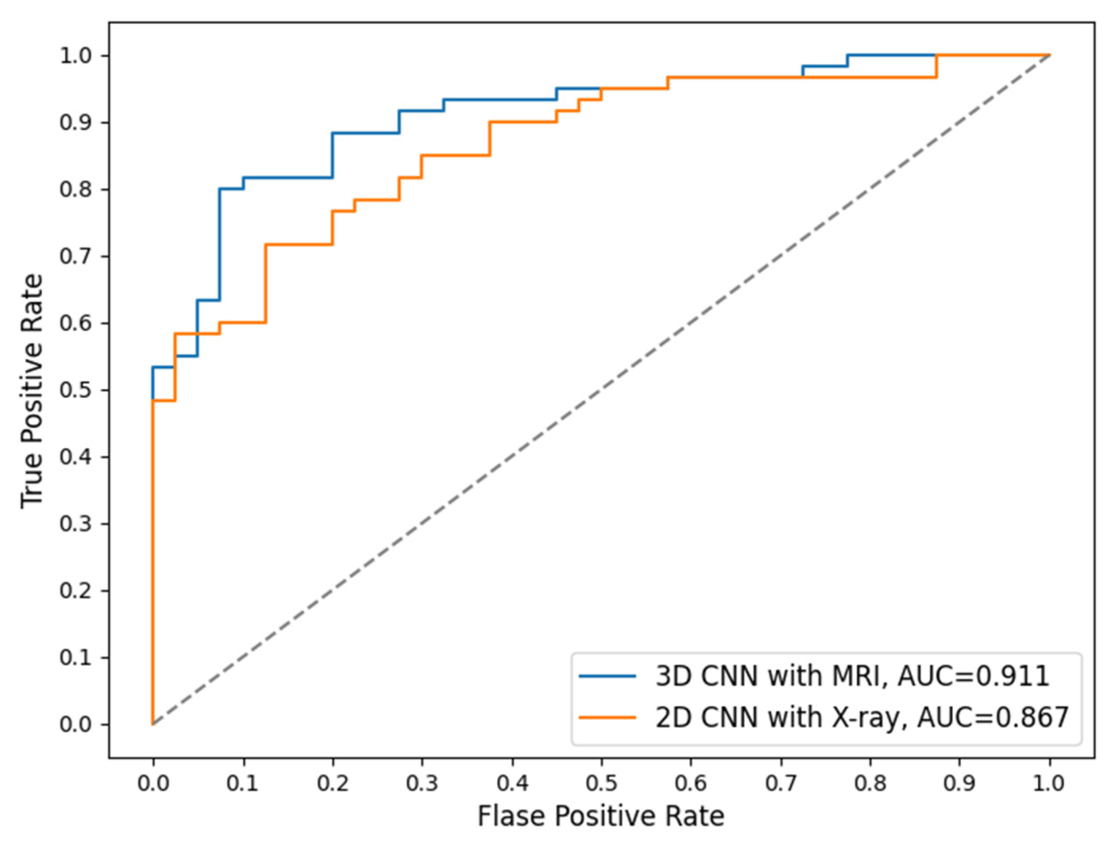
Currently, X-ray is the basic routine imaging modality for examining a patient with OA potentials clinically. While X-ray is more cost-efficient than MRI, it is not as sensitive as MRI, which can show much more structure and tissue details. Therefore, MRI is considered as an alternative imaging tool, especially for detecting early osteoarthritis with slight structure change.

In the 5-category results of this study we found that MRI had higher accuracy in classifying KL = 0 and KL = 1 (Table 6). This aligns with the previous studies that found MRI to be better at capturing detailed and small structure change and therefore more sensitive to early signs of OA development. When classifying the category KL = 4, X-rays have higher accuracy than MRI, indicating that X-rays are better at detecting OA in a more severe situation. The 2-category results in this study were consistent with those in the 5-category, in that X-ray has higher accuracy for detecting severe OA cases while MRI is more sensitive to small structure changes and early indicators of OA (Table 7). The complementary performance of the two imaging modalities is interesting and indicates the possibility that they could be combined to develop a comprehensive and more accurate diagnosis system than using each individual imaging modality alone.

A limitation of this study is that we have a limited number of samples. This is because we have to include patients with both MRI and X-ray scanned on the same knee. Another limitation is that MRI is not widely used in clinical diagnosis due to the cost. However, MRI is a new trend of imaging to study the pathology of knee OA in many clinical trials since MRI can offer a better view of soft tissues such as cartilage, bone marrow lesions, and effusions.

Future work includes further examination of the KL categories with lower accuracy, e.g., the KL = 2 category, which was often misclassified into KL = 1 (non-OA) by the model. This may be solved with a weighting system during training. Additionally, our current preprocessing uses a fixed offset for cropping as well as a fixed range for slice removing. This could be updated as a dynamic setting for each sequence, which may retrieve more accurate information and therefore generate better classification performance. Combining the two imaging modalities for a comprehensive and more accurate model is also a promising direction.

5. Conclusions

In this study, we proposed a novel 3D CNN model coupled with 3D MRI for knee OA classification. Guided by clinical knowledge, we reduced the input dimensionality of each image sequence by using subregions of MR images and removing less informative slices. Our model achieved an 83.0% accuracy in the OA/non-OA classification and a 54.0% accuracy in the 5-category KL grade classification. In addition, the F1 score and AUC for OA/non-OA classification are 0.831 and 0.911, respectively. Compared with using X-ray images coupled with classic 2D CNN architectures to classify knee OA for the same group of patients, the accuracy of both a 5-category KL grade classification and the 2-category OA/non-OA classification greatly improved. This indicates that more accurate knee OA diagnosis can be achieved using MR images coupled with 3D CNN models than using the traditional X-ray images and 2D CNN models.

References

1. Zhang, Y.; Jordan, J.M. Epidemiology of osteoarthritis. Clin. Geriatr. Med. 2010, 26, 355–369. [Google Scholar] [CrossRef] [PubMed] [Green Version]
2. Fransen, M.; McConnell, S.; Harmer, A.R.; Van der Esch, M.; Simic, M.; Bennell, K.L. Exercise for osteoarthritis of the knee: A Cochrane systematic review. Br. J. Sports Med. 2015, 49, 1554–1557. [Google Scholar] [CrossRef] [PubMed]
3. Felson, D.T.; Naimark, A.; Anderson, J.; Kazis, L.; Castelli, W.; Meenan, R.F. The prevalence of knee osteoarthritis in the elderly. The Framingham Osteoarthritis Study. Arthritis Rheum. Off. J. Am. Coll. Rheumatol. 1987, 30, 914–918. [Google Scholar] [CrossRef] [PubMed]
4. Jones, G.; Ding, C.; Scott, F.; Glisson, M.; Cicuttini, F. Early radiographic osteoarthritis is associated with substantial changes in cartilage volume and tibial bone surface area in both males and females. Osteoarthr. Cartil. 2004, 12, 169–174. [Google Scholar] [CrossRef] [PubMed] [Green Version]
5. Li, G.; Yin, J.; Gao, J.; Cheng, T.S.; Pavlos, N.J.; Zhang, C.; Zheng, M.H. Subchondral bone in osteoarthritis: Insight into risk factors and microstructural changes. Arthritis Res. Ther. 2013, 15, 223. [Google Scholar] [CrossRef] [PubMed] [Green Version]
6. Bhatia, D.; Bejarano, T.; Novo, M. Current interventions in the management of knee osteoarthritis. J. Pharm. Bioallied Sci. 2013, 5, 30–38. [Google Scholar] [CrossRef] [PubMed]
7. Kraus, V.B.; Nevitt, M.; Sandell, L.J. Summary of the OA biomarkers workshop 2009—Biochemical biomarkers: Biology, validation, and clinical studies. Osteoarthr. Cartil. 2010, 18, 742–745. [Google Scholar] [CrossRef] [PubMed] [Green Version]
8. Monti, S.; Montecucco, C.; Bugatti, S.; Caporali, R. Rheumatoid arthritis treatment: The earlier the better to prevent joint damage. RMD Open 2015, 1 (Suppl. 1), e000057. [Google Scholar] [CrossRef] [PubMed] [Green Version]
9. Eckstein, F.; Guermazi, A.; Gold, G.; Duryea, J.; Hellio Le Graverand, M.P.; Wirth, W.; Miller, C.G. Imaging of cartilage and bone: Promises and pitfalls in clinical trials of osteoarthritis. Osteoarthr. Cartil. 2014, 22, 1516–1532. [Google Scholar] [CrossRef] [PubMed] [Green Version]
10. Roemer, F.W.; Kwoh, C.K.; Hayashi, D.; Felson, D.T.; Guermazi, A. The role of radiography and MRI for eligibility assessment in DMOAD trials of knee OA. Nat. Rev. Rheumatol. 2018, 14, 372–380. [Google Scholar] [CrossRef] [PubMed]
11. Juras, V.; Chang, G.; Regatte, R.R. Current status of functional MRI of osteoarthritis for diagnosis and prognosis. Curr. Opin. Rheumatol. 2020, 32, 102. [Google Scholar] [CrossRef] [PubMed]
12. Peterfy, C.G.; Schneider, E.; Nevitt, M. The osteoarthritis initiative: Report on the design rationale for the magnetic resonance imaging protocol for the knee. Osteoarthr. Cartil. 2008, 16, 1433–1441. [Google Scholar] [CrossRef] [PubMed] [Green Version]
13. Hayashi, D.; Guermazi, A.; Roemer, F.W. MRI of osteoarthritis: The challenges of definition and quantification. In Seminars in Musculoskeletal Radiology; Thieme Medical Publishers: New York, NY, USA, 2012; Volume 16, pp. 419–430. [Google Scholar]
14. LeCun, Y.; Kavukcuoglu, K.; Farabet, C. Convolutional networks and applications in vision. In Proceedings of the 2010 IEEE International Symposium on Circuits and Systems, Paris, France, 30 May–2 June 2010; IEEE: Piscataway, NJ, USA, 2010; pp. 253–256. [Google Scholar]
15. Antony, J.; McGuinness, K.; O’Connor, N.E.; Moran, K. Quantifying radiographic knee osteoarthritis severity using deep convolutional neural networks. In Proceedings of the 2016 23rd International Conference on Pattern Recognition (ICPR), Cancún, Mexico, 4–8 December 2016; IEEE: Piscataway, NJ, USA, 2016; pp. 1195–1200. [Google Scholar]
16. Antony, J.; McGuinness, K.; Moran, K.; O’Connor, N.E. Automatic detection of knee joints and quantification of knee osteoarthritis severity using convolutional neural networks. In Proceedings of the International Conference on Machine Learning and Data Mining in Pattern Recognition, New York, NY, USA, 15–19 July 2017; Springer: Cham, Switzerland, 2017; pp. 376–390. [Google Scholar]
17. Górriz, M.; Antony, J.; McGuinness, K.; Giró-i-Nieto, X.; O’Connor, N.E. Assessing Knee OA Severity with CNN attention-based end-to-end architectures. arXiv 2019, arXiv:1908.08856. [Google Scholar]
18. Wahyuningrum, R.T.; Anifah, L.; Purnama, I.K.E.; Purnomo, M.H. A New Approach to Classify Knee Osteoarthritis Severity from Radiographic Images based on CNN-LSTM Method. In Proceedings of the 2019 IEEE 10th International Conference on Awareness Science and Technology (iCAST), Morioka, Japan, 23–25 October 2019; IEEE: Piscataway, NJ, USA, 2019; pp. 1–6. [Google Scholar]
19. Qi, C.R.; Su, H.; Nießner, M.; Dai, A.; Yan, M.; Guibas, L.J. Volumetric and multi-view cnns for object classification on 3d data. In Proceedings of the IEEE Conference on Computer Vision and Pattern Recognition, Las Vegas, NV, USA, 26 June–1 July 2016; pp. 5648–5656. [Google Scholar]
20. Dey, R.; Lu, Z.; Hong, Y. Diagnostic classification of lung nodules using 3D neural networks. In Proceedings of the 2018 IEEE 15th International Symposium on Biomedical Imaging (ISBI 2018), Washington, DC, USA, 4–7 April 2018; IEEE: Piscataway, NJ, USA, 2018; pp. 774–778. [Google Scholar]
21. Wang, T.; Leung, K.; Cho, K.; Chang, G.; Deniz, C.M. Total Knee Replacement prediction using Structural MRIs and 3D Convolutional Neural Networks. In Proceedings of the International Conference on Medical Imaging with Deep Learning—Extended Abstract Track, London, UK, 8–10 July 2019. [Google Scholar]
22. Pedoia, V.; Norman, B.; Mehany, S.N.; Bucknor, M.D.; Link, T.M.; Majumdar, S. 3D convolutional neural networks for detection and severity staging of meniscus and PFJ cartilage morphological degenerative changes in osteoarthritis and anterior cruciate ligament subjects. J. Magn. Reson. Imaging 2019, 49, 400–410. [Google Scholar] [CrossRef] [PubMed]
23. Astuto, B.; Flament, I.; Namiri, N.K.; Shah, R.; Bharadwaj, U.; Link, T.M.; Bucknor, M.D.; Pedoia, V.; Majumdar, S. Automatic deep learning assisted detection and grading of abnormalities in knee MRI studies. Radiol. Artif. Intell. 2021, 3, e200165. [Google Scholar] [CrossRef]
24. Raj, A.; Vishwanathan, S.; Ajani, B.; Krishnan, K.; Agarwal, H. Automatic knee cartilage segmentation using fully volumetric convolutional neural networks for evaluation of osteoarthritis. In Proceedings of the 2018 IEEE 15th International Symposium on Biomedical Imaging (ISBI 2018), Washington, DC, USA, 4–7 April 2018; IEEE: Piscataway, NJ, USA, 2018; pp. 851–854. [Google Scholar]
25. Kamnitsas, K.; Chen, L.; Ledig, C.; Rueckert, D.; Glocker, B. Multi-scale 3D convolutional neural networks for lesion segmentation in brain MRI. Ischemic Stroke Lesion Segm. 2015, 13, 46. [Google Scholar]
26. Chicco, D. Ten quick tips for machine learning in computational biology. BioData Min. 2017, 10, 1–17. [Google Scholar] [CrossRef] [PubMed]
27. Ripley, B.D. Pattern Recognition and Neural Networks; Cambridge University Press: Cambridge, UK, 2007. [Google Scholar]
28. He, K.; Zhang, X.; Ren, S.; Sun, J. Deep residual learning for image recognition. In Proceedings of the IEEE Conference on Computer Vision and Pattern Recognition, Las Vegas, NV, USA, 26 June–1 July 2016; pp. 770–778. [Google Scholar]
29. Simonyan, K.; Zisserman, A. Very deep convolutional networks for large-scale image recognition. arXiv 2014, arXiv:1409.1556. [Google Scholar]
30. Szegedy, C.; Vanhoucke, V.; Ioffe, S.; Shlens, J.; Wojna, Z. Rethinking the inception architecture for computer vision. In Proceedings of the IEEE Conference on Computer Vision and Pattern Recognition, Las Vegas, NV, USA, 26 June–1 July 2016; pp. 2818–2826. [Google Scholar]
31. Szegedy, C.; Ioffe, S.; Vanhoucke, V.; Alemi, A. Inception-v4, inception-resnet and the impact of residual connections on learning. arXiv 2016, arXiv:1602.07261. [Google Scholar]
32. Huang, G.; Liu, Z.; Van Der Maaten, L.; Weinberger, K.Q. Densely connected convolutional networks. In Proceedings of the IEEE Conference on Computer Vision and Pattern recognition, Honolulu, HI, USA, 21–26 July 2017; pp. 4700–4708. [Google Scholar]
Figure 1. Overview of the models proposed in this study. The input data for each patient are a sequence of MR images. Each sequence is preprocessed by cropping and then removing slices. This reduced data are fed into a 3D CNN. The second pipeline applies the same 3D CNN architecture but is trained separately for the binary OA/non-OA classification.
Applsci 11 05196 g001
Figure 2. A 2D slice from a 3D knee MR image sequence. The circled area is the cartilage region between the femur and tibia bones.
Applsci 11 05196 g002
Figure 3. A full 384 × 384 image and the results of cropping to various window sizes.
Applsci 11 05196 g003
Figure 4. A selection of 4 slices from a set of 160 MR images for a single patient’s left knee.
Applsci 11 05196 g004
Figure 5. The architecture of the 3D CNN model used in this study. Details of the convolutional block and the identity block are shown in Figure 6.
Applsci 11 05196 g005
Figure 6. Details of the convolutional block and the identity block.
Applsci 11 05196 g006
Figure 7. ROC curves for the OA/non-OA classification.
Applsci 11 05196 g007