Grounding Electrodes with Internal Resistance: Application to Feasibility Study of the Driven-Rod Method for Modeling the Soil Electrical Resistivity Profile

Featured Application

The model proposed in the paper can be applied to any electrode to assess the impact of its internal resistance on the main parameters that define a grounding system.

Abstract

The paper presents a model to include the internal resistance of the grounding electrodes in the calculation of its electrical features. The semi-analytical expressions for the calculation of the grounding resistance arising from the model are used to study the feasibility of the driven-rod method for the estimation of the soil resistivity profile since, unlike other methods, the internal resistance of the conductors can be of great influence for a correct estimate. From the grounding resistance profile an inverse problem based on the minimization of the quadratic differences between the resistance measured and that calculated from the model is posed. Several synthetic examples are used to assess the limitations of the method in conditions close to real situations. Finally, some real cases involving data measured in the field are analyzed. Whether in synthetic examples or in real soils it is found that the spatial frequency of the driven-rod resistance sampling is a determinant factor in order to study the feasibility of the driven–rod method.

1. Introduction

The estimation of the soil resistivity as a function of the depth is a key point for modelling any grounding system [1]. There are several methods to determine the soil resistivity. Most of them are indirect methods that use an intermediate magnitude as the apparent resistivity. In one of the most used methods, the resistivity is estimated from a vertical electrical sounding (VES) performed with a four-pin device as in the Wenner and Schlumberger arrays, from which the apparent resistivity is obtained [2]. From the apparent resistivity, it is possible to find out the soil resistivity profile, provided that a constant multi-layered model has been adopted [3,4]. Even though the VES is a non-invasive procedure, small errors in the measuring procedure could lead to a soil model far from the real one. The ill-conditioned nature of the method to obtain the resistivity profile from the soil’s apparent resistivity is at the bottom of the issue [5,6]. On the other hand, in some sense a VES could be seen as a non-local test since the soil conductivity between the active electrodes of the test array is being checked. Note for instance that in a Wenner array the active electrodes are separated three times the distance between adjacent probes. The soil properties could change horizontally leading to a soil resistivity profile that would not match with the real one. This is especially important when a grounding system makes use of vertical rods as grounding electrodes, such as in the case of lightning protection electrodes.

Another indirect procedure sometimes used is the driven-rod method. In this method, the grounding resistance of a rod driven into the ground is measured by the fall-of-potential procedure [7]. If the rod is modeled as a cylinder of length L and radius r, where L >> r and with a hemisphere at the end, the grounding resistance in a homogeneous medium of resistivity, rho, is $R=\frac{\rho }{2\pi L}\ln (\frac{2L}{d})$. On the other hand, if the rod is modeled as a half-ellipsoid of revolution, whose major axis is L and its minor axis is the diameter d, the expression $R=\frac{\rho }{2\pi L}\ln (\frac{4L}{d})$ must be used. 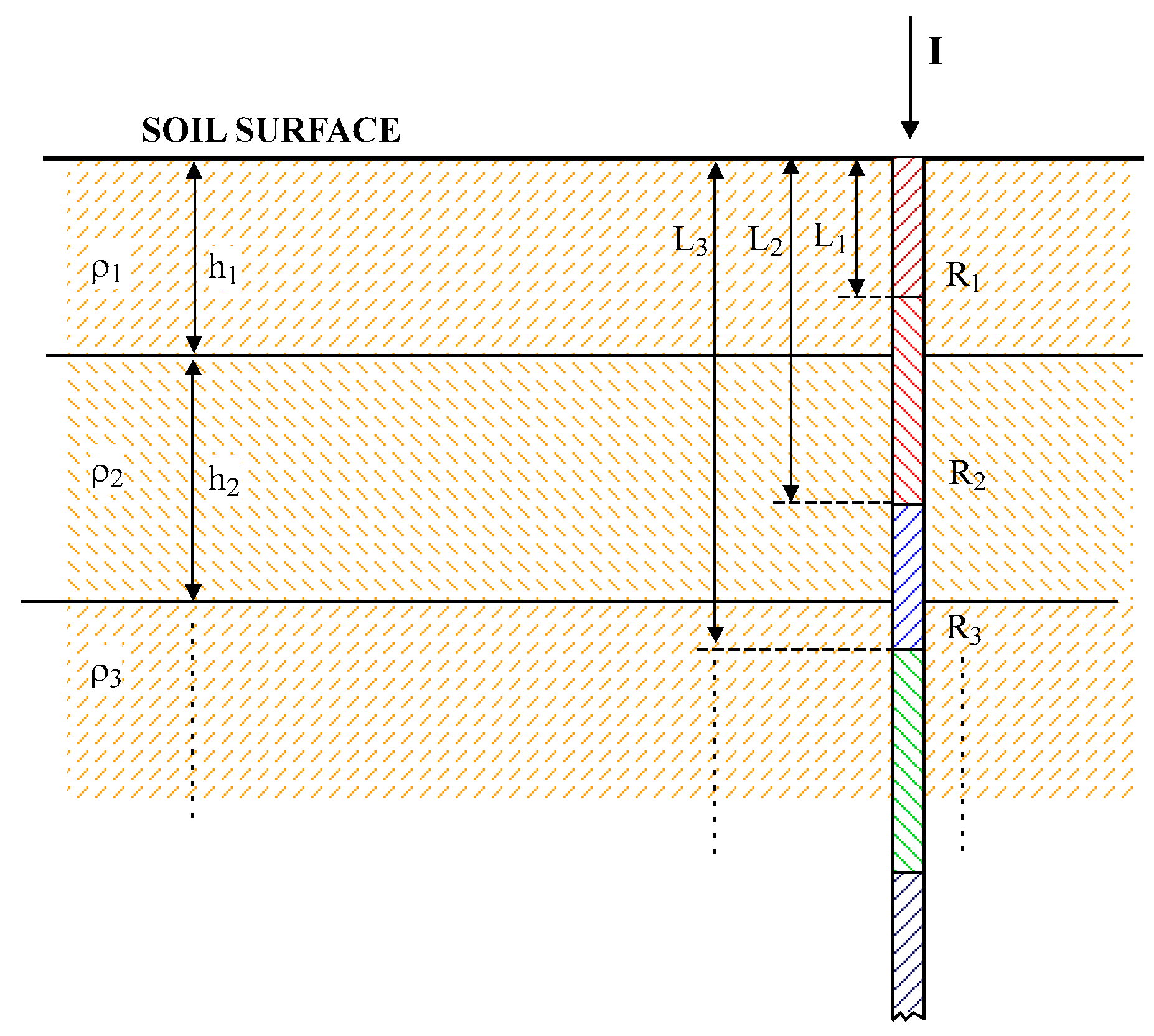Another expression widely used to theoretically estimate grounding resistance is $R=\frac{\rho }{2\pi L}[\ln (\frac{8L}{d})-1]$ [8] in which the supplementary assumption is made that the ground leakage current has a constant distribution along the rod. By varying the length of the rod, an apparent resistivity profile ${\rho }_{app}(L)$ representing the resistivity seen by the rod of length L can be obtained. Figure 1 outlines the data that are necessary to implement the method. An advantage of the driven-rod method is that it allows obtaining valuable information on the feasibility of a grounding system. Knowing the necessary depth to obtain a given grounding resistance could greatly facilitate the final touch-up of the grounding system design.

An important observation is that the above mentioned VES method is not very sensitive to the state or type of electrodes used except for a shallow depth where the electrodes are very close together and their size and shape influence somewhat the potential [9]. In general, it does not matter if the electrodes are corroded or if they have a great internal resistance since what is measured is a potential difference on the ground. In contrast, the driven-rod method is greatly affected by oxidation and the internal resistance of the rod. The previous expressions for the grounding resistance R as a function of the rod length L, were found under the condition that the rods are ideal conductors without internal resistance. Therefore, it is to be expected that this fact will need to be taken into account when looking for a model for soil resistivity. There are more reasons, in addition to those already exposed, to incorporate the internal resistance of the conductors into the calculation scheme of the electrical properties of a grounding electrode. The current trend of using materials with non-negligible internal resistance such as carbon steel or others for the electrodes of a grounding system makes it necessary to study their effect on the parameters of the system. After setting a calculation model for the electrodes that takes into account their internal resistance, the here called Resistive Driven-Rod method (RDR), which takes into account the internal resistance of the rod will be applied both to synthetic and real soils.

A direct method to determine the resistivity as a function of the depth is known in literature as normal resistivity logging (NRL) [10]. This is a geophysical method for determining the rock’s conductivity by studying the drilling geological profile in a well. However, this technique requires the drilling of a well of a section large enough for the probes to be introduced. Resistivity is measured with a four-pin device taking a short electrode separation so that the well walls can be tested. To complete this brief review of several of the methods used to investigate the electrical structure of soils, mention should be made of the magnetic field-based eddy-current methods (ECM), framed in the transient electromagnetic methods class. By means of a coil near the soil surface, a variable magnetic field is produced. Eddy-currents are generated in the conductive soil, producing magnetic fields that depend on the layer structure. Although they are based on very different principles from those of the methods described so far, ECM are clearly non-invasive methods with high resolution at shallow depth [11].

From the apparent resistivity data obtained with the indirect methods described above, the soil resistivity profile can be obtained by posing an inverse problem. Starting from semi-analytical expressions for the grounding resistance as a function of the parameters of a multilayer model, an optimization algorithm is implemented to find the set of parameters of the model that minimizes the squared differences between the values of the resistance measured in the field and those calculated with the theoretical expressions that contain the parameters. However, the techniques used in the inverse problem with the measurements made with the Wenner array cannot be extended when the measurements come from a driven-rod logging. Apparent resistivity has a different meaning depending on the type of measurement.

The main objectives of this paper are, firstly, to establish a systematic procedure to include the internal resistance of conductors in the calculation of the grounding resistance of buried electrodes, and secondly, testing the feasibility of the RDR method to determine the parameters of a multilayer soil model from grounding resistance measurements, pointing out its limitations. To achieve these goals, the paper is structured as follows. After the present introduction, the backgrounds section is intended to introduce the foundations of the proposed method. In the next section, some tests are carried out on synthetic soils in order to test the method relevance. In the same section some real examples are also studied. Finally, the conclusions of the work are collected in the last section.

2. Modeling Grounding Electrodes with Internal Resistance: Backgrounds

The calculation of the grounding resistance of an electrode needs the model for the electrical conductivity of the soil to be known. From a general point of view, it would be necessary to solve the equation $\overrightarrow{\nabla }\cdot (\sigma (\overrightarrow{r})\overrightarrow{\nabla }\varphi (\overrightarrow{r}))=0$ together with some boundary conditions, where $\varphi (\overrightarrow{r})$ is the absolute potential at the point $\overrightarrow{r}$ and $\sigma (\overrightarrow{r})$ represents the conductivity of the ground. For a multilayered model it is possible to find acceptable semi-analytical solutions for the potential. This model assumes that conductivity is just a non-continuous piecewise constant function. The soil is composed of horizontal layers of infinite extension and specific thickness in which the electrical conductivity takes a constant and different value in each layer. Thus, the actual conductivity is replaced by a step function although in practice, due to the difficulty of the calculations, only a few layers are considered. The soil conductivity profiles of interest for this work comprise layers of almost any conductivity with thicknesses ranging from a few centimeters to tens of meters. Although for applications in grounding design it is common to deal with models in which the top layer is a few meters thick in which to place the grounding electrode.

Choosing a constant conductivity in each layer allows calculating the potential from the equation for a generic conductivity. The connection between the solutions corresponding to each layer is made by imposing the continuity of the potential at the different interfaces as well as the continuity of the normal component of the current density through interfaces.

Due to the supposed cylindrical symmetry of the potential, which is associated with conductivity dependent only on the depth as the z coordinate, the procedure to solve the equation for the potential relies on using the method of separation of variables in a cylindrical coordinate system. Thus, the potential created in layer j by an electric point current source of strength I in layer i could be written as [12]

$${\varphi }_{ij}=\frac{{\rho }_{i}I}{4\pi \left|{\overrightarrow{r}}_i-{\overrightarrow{r}}_j\right|}{\delta }_{ij}+{\displaystyle \underset{0}{\overset{\infty }{\int }}(f_{ij}(\lambda )e^{-\lambda (z_i-z_j)}+g_{ij}(\lambda )}{e}^{\lambda (z_i-z_j)})J_0(\lambda r)d\lambda$$

(1)

where ${\delta }_{ij}$ is the Kronecker delta and the unknown functions $f_{ij}$ and $g_{ij}$ need to be calculated by imposing the boundary conditions at each interface, namely $\overrightarrow{\nabla }{\varphi }_{i1}\cdot {\overrightarrow{n}}_z|{}_{z=0}=0$ which stands for the null current flux through the soil surface and

$$\begin{array}{l}{\varphi }_{ij}({\overrightarrow{r}}_{j,j+1})={\varphi }_{ij+1}({\overrightarrow{r}}_{j,j+1})\\ {\sigma }_j\cdot \overrightarrow{\nabla }{\varphi }_{ij}\cdot \overrightarrow{n}|{}_{{\overrightarrow{r}}_{j,j+1}}={\sigma }_{j+1}\cdot \overrightarrow{\nabla }{\varphi }_{ij+1}\cdot \overrightarrow{n}|{}_{{\overrightarrow{r}}_{j,j+1}}\end{array}$$

(2)

what guarantees continuity of potential and normal current flux conservation through the interface separating the layers j and j + 1. In (1) and (2), ${\rho }_i$, is the constant resistivity of layer i, $r=\sqrt{{(x_i-x_j)}^2+{(y_i-y_j)}^2}$ and $J_0$ is the zero-order Bessel function. In (1) the functions$f_{ij}(\lambda )$ and $g_{ij}(\lambda )$ must be calculated by (2) at the above-mentioned interfaces. The calculation of the functions f and g can be difficult and the evaluation of the integral in (1) is only approximate due to the oscillatory character of the $J_0$ Bessel function, in addition to the own singularities of the f and g functions [13].

In order to properly implement the boundary conditions (2), it is necessary to convert the first term on the right hand of (7) to an integral form so that the entire expression is in an integral form. The integral forms of Lipschitz (3), allow such a conversion to be carried out [14],

$$\begin{array}{l}\frac{1}{\left|\overrightarrow{r}-{\overrightarrow{r}}_P\right|}={\displaystyle \underset{0}{\overset{\infty }{\int }}{e}^{-\lambda \cdot \left|z-z_P\right|}}{J}_0(r\lambda )d\lambda \\ \end{array}$$

(3)

Thus, the boundary conditions (2) lead to a linear system in the unknowns $f_{ij}$ and $g_{ij}$ that is solved by symbolic calculus using the software Wolfram Mathematica.

The point current source potentials (1), serve as the basis for calculating the grounding resistance of any electrode, particularly a rod driven into the soil. If it is a perfectly conductive rod, the potential can be calculated using the superposition law and the grounding resistance, as well as the step and touch potentials can be obtained. Indeed, the expression (1) stands for the potential generated by a single point current source. When an extended electrode leaking a fault current to the ground is considered, expressions like (1) can be used under some conditions imposed on the electrodes. The electrodes are assumed as composed by thin wire pieces assembled to form the entire electrode. Thus, each thin wire could be considered as a distribution of point current sources located in the axis. The potential at point $\overrightarrow{r}$ of the layer j generated by a thin wire of length L located in the layer i, is given by

$$\begin{array}{l}{\varphi }_{ij}(\overrightarrow{r})={\displaystyle \underset{L}{\int }\frac{{\rho }_i\cdot \mu ({\overrightarrow{r}}_P)}{4\pi \left|\overrightarrow{r}-{\overrightarrow{r}}_P\right|}d{l}_P\cdot {\delta }_{ij}}+\\ +{\displaystyle \underset{L}{\int }\frac{{\rho }_i\cdot \mu ({\overrightarrow{r}}_P)}{4\pi }[{\displaystyle \underset{0}{\overset{\infty }{\int }}({\widehat{f}}_{ij}(\lambda )e^{-\lambda (z-z_P)}+}{\widehat{g}}_{ij}(\lambda )e^{\lambda (z-z_P)})J_0(\lambda r)d\lambda }]d{l}_P\end{array}$$

(4)

where $\mu ({\overrightarrow{r}}_P)$ stands for the point current sources density along the thin wire axis and the functions ${\widehat{f}}_{ij}$and ${\widehat{g}}_{ij}$ need to be calculated, again imposing the boundary conditions at each interface. A more general situation could take place when the thin wire is between several layers at the same time. In practice, the thin wire is segmented in M short pieces of length $\Delta l_m$ each of them with constant point current sources density ${\left\{{\mu }_m\right\}}_{m=1\cdots M}$, which are used to calculate the potential of the electrode itself by imposing a constant value of such potential along the entire electrode, the grounding electrode potential [15]. Thus, the potential at point $\overrightarrow{r}$ of the layer j becomes:

$$\begin{array}{l}\varphi ({\overrightarrow{r}}_j)={\displaystyle \sum _{m=1}^M\frac{{\rho }_m\cdot {\mu }_m\cdot \Delta l_m}{4\pi \left|{\overrightarrow{r}}_j-{\overrightarrow{r}}_m\right|}{\delta }_{mj}}+\\ +{\displaystyle \sum _{m=1}^M\frac{{\rho }_m\cdot {\mu }_m\cdot \Delta l_m}{4\pi }}{\displaystyle \underset{0}{\overset{\infty }{\int }}({\widehat{f}}_{mj}(\lambda )e^{-\lambda (z_j-z_m)}+}{\widehat{g}}_{mj}(\lambda )e^{\lambda (z_j-z_m)})J_0(\lambda r)d\lambda \end{array}$$

(5)

This procedure, known as moment method, gives rise to a system of linear equations whose unknowns are the constant densities ${\left\{{\mu }_m\right\}}_{m=1\cdots M}$ of point current sources in each segment [16]. The knowledge of these densities allows the calculation of the potential at any point on the ground by superposition. The electrode potential itself is of special interest for this work. As it was pointed out, it is obtained as a part of the solution for the ${\mu }_k$ densities and then the grounding resistance can be easily calculated.

When the electrode is a conductor with non-zero internal resistance, the calculation of the potential acquired by the electrode is somewhat more complicated since it is no longer equipotential. In this case, the electrode potential is commonly measured at the current injection point which is the point of the electrode where the fault current to be leaked to the ground enters. Usually, for electrodes with non-negligible internal resistance, both the current injection point and the measurement point are important parameters since the potential value is strongly dependent on the internal distribution of leakage currents to the ground. With respect to the model used to take into account the internal resistance of the electrodes, the one used here is the Circuit-Based Model (CBM) [17,18]. According to this model, the electrodes are broken down into branches and nodes to which circuit theory applies. Figure 2 shows in the upper part a rod like the ones used in the driven-rod test, which is divided into N branches. The potential U_k and the leakage current I_k in each branch are displayed. At the bottom, the circuit-based model is shown. At each node of the circuit, the potential V_t and the source of nodal leakage current J_t are located. The internal currents i_k that move inside the conductor are also shown.

Each branch obeys a general equation for the potential difference between the ends (nodes) that for the generic branch k takes the form,

$$V_{k^{+}}-V_{k^{-}}=i_k\cdot z_k+{\displaystyle \sum _{r=1}^B{i}_r\cdot Z_{kr}^L}$$

(6)

where B is the number of branches of the electrode system containing N nodes, i_r is the current through the branch r, z_k is the internal resistance of the branch k and $Z_{kr}^L$ is the inductive impedance of the branch k due to the branch r (sometimes called longitudinal impedance), which can be neglected for stationary or low frequency currents. Figure 3 shows a diagram of the magnitudes introduced for a branch of the circuit.

The branch currents i_k and the node currents J_n are related by Kirchhoff’s law: for the node n, the algebraic sum of all currents that concur in the node is zero, ${\displaystyle \sum _n{i}_k+J_n+F_n=0}$, where the possible source or injection currents F_n on the node n have been introduced. This expression must be introduced in (6) so that only the currents and potentials of node, J_n and V_n respectively, together with the supply currents F_n, are considered as the main variables.

To establish the relationship between the currents in the nodes, it is necessary to agree on a consistent sign criterion. It will be agreed to consider positive the outgoing currents of the nodes either towards the branches, i_k, or towards the ground, J_n, and the potential differences between the nodes of each branch will be evaluated from the node through which the current leaves until the node through which it enters. Using this convention, it can be written:

$$J_k+{\displaystyle \sum _{l=1}^N{G}_{lk}\cdot V_l=F_k}(k=1\cdots N)$$

(7)

The square matrix G is constructed from Kirchhoff’s law in each node, Ohm’s law in each branch and the branch-node connection matrices, all together with the coherent criterion of signs for the currents.

At the same time that a potential difference due to the internal circulation of branch currents is generated in each branch, an absolute potential (with respect to the null potential of infinity) is also generated in each branch due to the leakage currents towards the surrounding conductive soil. Thus, each branch acquires a potential U_k, which depends on the currents filtered to the ground by all other branches I_m, including the branch k itself. Thus, it can be stated

$$U_k={\displaystyle \sum _{m=1}^B{I}_m\cdot Z_{km}}$$

(8)

where the impedance Z_km (sometimes called transverse impedance [19]) has the following expression for a multi-layered soil,

$$Z_{km}=\frac{{\rho }_m}{4\pi }{\displaystyle \underset{l_m}{\int }d{l}_m}\left[\frac{1}{\left|{\overrightarrow{r}}_k-{\overrightarrow{r}}_m\right|}{\delta }_{km}+{\displaystyle \underset{0}{\overset{\infty }{\int }}(f_{km}(\lambda )e^{-\lambda (z_k-z_m)}+g_{km}(\lambda )}{e}^{\lambda (z_k-z_m)})J_0(\lambda r)d\lambda \right]$$

(9)

The expressions (8) and (9) are completely equivalent to (5) with $I_m={\mu }_m\cdot \Delta l_m$. Moreover, ${\rho }_m$ is the soil resistivity around the branch m and as it was already mentioned before, the functions $f(\lambda )$ and $g(\lambda )$ are calculated by imposing the boundary conditions at each interface [12].

From the expressions (8) and (9) it is shown that the absolute potential acquired by the branch k as a result of the current filtered to the ground, can be put in the matrix form ${(U)}_{B,1}={(Z_T)}_{B,B}{(I)}_{B,1}$, where the subscripts indicate the dimension of the matrices (B will denote the number of branches and N will denote the number of nodes) and the square matrix (Z_T) is the matrix of transverse impedances.

For a proper application of circuit analysis, it is necessary to establish a relationship between leakage currents and potentials in the branches and nodes. In Figure 3, two types of currents are shown, the leakage current of the branch I_i and those that go from the nodes of the branch J_k+ y J_k-, both towards the surrounding medium. It will be agreed that both node and branch currents to the surrounding medium are related by the matrix equation

$${\left(J\right)}_{N,1}={(C)}_{N,B}\cdot {(I)}_{B,1}$$

(10)

where (C) is a matrix of N rows (nodes) and B columns (branches) whose elements are

$$c_{ij}=\{\begin{array}{l}1/2\mathrm{if}\mathrm{the}\mathrm{node}\mathrm{i}\mathrm{is}\mathrm{connected}\mathrm{to}\mathrm{the}\mathrm{branch}\mathrm{j}\\ 0\mathrm{otherwise}\end{array}$$

(11)

This means that each branch leakage current I_i is divided into two halves that go to the currents of nodes $J_{i^{+}}$ and $J_{i^{-}}$. With regard to the branch potential U_i and the potentials of the branch nodes V_i⁺ and V_i^-,

$${\left(U\right)}_{B,1}={(K)}_{B,N}\cdot {(V)}_{N,1}$$

(12)

with (K) being a matrix of B rows (branches) and N columns (nodes), whose elements are

$$k_{ij}=\{\begin{array}{l}1/2\mathrm{if}\mathrm{the}\mathrm{branch}\mathrm{i}\mathrm{is}\mathrm{connected}\mathrm{to}\mathrm{the}\mathrm{node}\mathrm{j}\\ 0\mathrm{otherwise}\end{array}$$

(13)

which really means that the branch potential is the average value of the potentials of its nodes $U_i=\frac{V_n+V_{n+1}}{2}$. With Equations (7), (8), (10) and (12) a system of matrix equations can be proposed,

$$\begin{array}{l}{(J)}_{N,1}+{(G)}_{N,N}\cdot {(V)}_{N,1}={(F)}_{N,1}\\ {(U)}_{B,1}={(Z)}_{B,B}\cdot {(I)}_{B,1}\\ {(J)}_{N,1}={(C)}_{N,B}\cdot {(I)}_{B,1}\\ {(U)}_{B,1}={(K)}_{B,N}\cdot {(V)}_{N,1}\end{array}$$

(14)

Defining a vector of unknowns consisting of currents and potentials I_n y V_n

$${(W)}_{B+N,1}=\left(\begin{array}{l}{(I)}_{B,1}\\ {(V)}_{N,1}\end{array}\right)$$

(15)

the system of Equation (14) can be written as

$$\left(\begin{array}{cc}{(Z)}_{B,B}& -{(K)}_{B,N}\\ {(C)}_{N,B}& {(G)}_{N,N}\end{array}\right)\cdot {(W)}_{N+B,1}=\left(\begin{array}{c}{(0)}_{B,1}\\ {(F)}_{N,1}\end{array}\right)$$

(16)

which allows us to find the solution of the problem in terms of potentials and currents.

The electrode potential is the one corresponding to the node through which the current enters the electrode and the grounding resistance is the quotient between this potential and the injected current. Note that both depend on the parameters of the multilayer model chosen through ${\rho }_m$ and the functions $f(\lambda )$ and $g(\lambda )$ in (9).

For an L length rod driven into the soil of parameters $\left\{{\rho }_1,{\rho }_2\dots ,h_1,h_2\dots \right\}$, the calculated grounding resistance will be denoted as $R_{calc}(L;\left\{{\rho }_1,{\rho }_2\dots ,h_1,h_2\dots \right\})$. In practice, a direct measurement in the field of the grounding resistance R_meas of the rod by the fall-of-potential method is performed. The control variable is the rod length L, thus a set of grounding resistance values corresponding to increasing lengths of the rod are available. From these measurements an optimization algorithm that minimizes

$${\chi }^2={\displaystyle \sum _j{[R_{meas}(L_j)-R_{calc}(L_j;\left\{{\rho }_1,{\rho }_2\dots ,h_1,h_2\dots \right\})]}^2}$$

(17)

could be implemented. This problem falls into the category of so-called inverse problems, which are very often ill-conditioned. That means in practice that uncertainties in the measurements of grounding resistance can led to very dramatic changes in the parameter values of the multilayered model. Consequently, there may be no single solution to the resistivity profile from the measured grounding resistance series.

To finish this section, some considerations about the model presented here will be discussed. The internal resistance of a grounding electrode plays an important role for several reasons. In the first place, as already mentioned, the electrode is no longer equipotential, and the grounding resistance must be defined as indicated above. The current injection point is an important choice and must be chosen so that its potential is as low as possible. Second, the calculations made with this model allow validating or discarding materials to be used in electrodes on condition of verifying technical requirements on the value of the grounding resistance and the step and touch potentials required in an installation. Note that increasing the size of the electrodes can help to decrease the grounding resistance as long as the internal resistance of the conductors does not result in a final increase in the grounding resistance. Finally, another effect to consider that can only be evaluated with models such as the one presented here is the heating by the Joule effect on the electrodes. The heat generated can cause an unwanted increase in grounding resistance when taking into account the variation in resistivity with temperature. The effect must be studied and only models that take into account the internal resistivity of the conductors are valid for this purpose.

3. Application to Resistive Driven-Rod Method: Testing with Some Examples

In the tests that will be described below, a rod is vertically driven into a multilayer soil and the grounding resistance is measured as a function of the length of the rod that is buried in the soil. According to the circuit-based model introduced in Section 2, each branch of the buried rod contributes with a leakage current leakage to the ground and electric potentials are generated at its ends that must be determined by solving (16). The grounding resistance can be calculated from the potential acquired by the injection point of the total current, which is usually the upper end of the rod. This potential depends on the internal resistance of the rod and the resistivity profile of the ground through the resistivity and width of the different layers. These soil parameters can be found by a minimization procedure of (17). In order to work in conditions similar to the real tests, some additional considerations need to be discussed.

First of all, it is necessary to comment that in many real cases, the rod driven into the soil is composed of rod segments of fixed length assembled by means of small joining pieces. Such connecting pieces provide a contact resistance between the two rods that are joined that makes the whole rod a conductor with non-zero internal resistance. This fact will be modeled by associating a non-zero resistivity to the connecting piece between the adjacent rods, the rods themselves being ideal conductors. Each time a rod segment is assembled with a joining piece and driven into the ground, the grounding resistance of the entire rod is measured. For practical reasons, the rod segments usually have a size ranging from 1 m to 1.5 m while the connecting pieces have a length of a few centimeters. In some of the synthetic cases that will be studied, 0.5 m rod segments will be used although this size is actually fictitious.

3.1. Synthetic Examples with No Internal Resistance

Let us consider first a synthetic example in which the rod has no internal resistance. Let the ground be a synthetic three-layer soil with parameters ρ₁ = 100 Ωm, ρ₂ = 50 Ωm, ρ₃ = 300 Ωm, h₁ = 2 m, and h₂ = 3 m, where a vertical zero-resistive rod of 9 mm radius is driven into the soil from 0.5 m up to 8 m deep. The rod is assumed to be made of a single continuous piece that is introduced in segments of 0.5 m in the ground. For every 0.5 m of drilling, the grounding resistance is calculated assuming that it is a value obtained in a field measurement using the fall-of-potential method.

Table 1. Buried rod length L (m) and the corresponding grounding resistance R (Ω).

L (m)	0.5	1	1.5	2	2.5	3	3.5	4
R (Ω)	139.90	80.67	57.79	44.68	31.74	25.52	21.66	19.05
L (m)	4.5	5	5.5	6	6.5	7	7.5	8.0
R (Ω)	17.18	15.97	15.76	15.54	15.31	15.07	14.85	14.62

shows the results where L is in meters and R is in Ohms.

From data of Table 1, a MatLab-based minimization algorithm using the fminsearch routine is launched where the objective function is (17). The parameters of the model obtained from the minimization procedure are ρ₁ = 99.01 Ωm, ρ₂ = 49.79 Ωm, ρ₃ = 292.45 Ωm, h₁ = 2.03 m, and h₂ = 2.94 m. Figure 4 shows by using diamond markers the values on the Table 1. The red continuous line, labeled as Calculated 1, stands for the calculated grounding resistance from the obtained optimum solution while the dashed blue line, labeled as Calculated 2, shows the calculated grounding resistance from the true soil parameters. The subfigure in Figure 4 stands for the percentage error ${\epsilon }_R=(R_{true}-R_{calc})/R_{true}$ in the calculation of the grounding resistance using the estimated soil model, where $R_{true}$ is the grounding resistance from the true soil model, whilst $R_{calc}$ is the calculated grounding resistance from the estimated soil model.

Although sixteen simulated data have been used in this synthetic example, it is possible to recover the soil structure with much less data. Let consider another example of synthetic soil ρ₁ = 50 Ωm, ρ₂ = 200 Ωm, ρ₃ = 10 Ωm, h₁ = 2 m, and h₂ = 3 m. Again, we will assume a non-zero internal resistance rod of 9 mm radius driven into the soil. As before, the rod is assumed to be made of a single continuous piece that is driven into the ground, but in this experiment the grounding resistance is simulated every 1.5 m. Only five grounding resistances corresponding to five buried electrode lengths will be simulated.

Table 2. Buried rod length L (m) and the corresponding grounding resistance R (Ω).

L (m)	1.5	3	4.5	6	7.5
R (Ω)	30.51	22.78	19.46	5.79	3.24

collects the simulated grounding resistance for the considered rod lengths.

The parameters of the model obtained from the minimization procedure are ρ₁ = 49.47 Ωm, ρ₂ = 171.76 Ωm, ρ₃ = 9.59 Ωm, h₁ = 1.85 m, and h₂ = 3.22 m, which shows significant differences with the values of the real soil, especially in the intermediate layer. However, the grounding resistance obtained for the five lengths considered is very close to its true value. Figure 5 shows with diamond markers the values on the Table 2. The red continuous line labeled as Calculated 1, stands for the calculated continuous grounding resistance from the solution of the minimization procedure. The blue line stands for the calculated continuous grounding resistance but using the true soil structure. The differences between the estimated soil structure and the actual structure come from coarse sampling of the soil when using the grounding resistance of the vertical rod in jumps of 1.5 m length. This effect is most obvious when there are large changes in resistivity between layers. The continuous red line in subfigure, labeled as E-Calculated 1, stands for the percentage of error ${\epsilon }_R=(R_{true}-R_{calc})/R_{true}$ in the calculation of the grounding resistance using the estimated soil model, which give rise to the above-mentioned curve labeled Calculated 1 in the main figure.

If the grounding resistance is now measured every time 0.5 m of rod driven into the ground, new data have to be added to Table 2 obtaining

Table 3. Buried rod length L (m) and the corresponding grounding resistance R (Ω).

L (m)	0.5	1	1.5	2	2.5	3	3.5	4
R (Ω)	71.11	41.63	30.51	25.10	24.01	22.78	21.66	20.53
L (m)	4.5	5	5.5	6	6.5	7	7.5	8.0
R (Ω)	19.46	18.12	8.21	5.79	4.55	3.77	3.24	2.85

.

The minimization procedure applied on data of Table 3 results in a set of soil parameters ρ₁ = 49.34 Ωm, ρ₂ = 217.28 Ωm, ρ₃ = 10.73 Ωm, h₁ = 1.95 m, and h₂ = 3.02 m, which give rise to the green dashed line labeled as Calculated 3 in Figure 5. Note that the calculated grounding resistance by the new optimum model is very close to that calculated by the true soil model since the values of the estimated soil parameters are very close to those of the actual soil. The continuous blue line, labeled as Calculated 2, stands for the grounding resistance profile from the improved resistivity model. The corresponding error ${\epsilon }_R=(R_{true}-R_{calc})/R_{true}$ is shown as E-Calculated 3 in the subfigure. As a conclusion, the larger the sample of grounding resistance data, the better the estimation of the soil model parameters.

3.2. Synthetic Examples with Internal Resistance

To finish the study of synthetic soils, a rod again 9 mm radius with non-zero internal resistance driven into the soil will be considered. Let us consider the synthetic soil ρ₁ = 100 Ωm, ρ₂ = 200 Ωm, ρ₃ = 40 Ωm, h₁ = 3 m, and h₂ = 1 m. In order to get closer to the real data that will be used as a test of the RDR method, suppose that sections 1.5 m long of galvanized-steel low-resistive rod ρ = 13.8 × 10⁻⁸ Ωm are assembled as shown in Figure 6. Let also suppose that the imperfect contact between the pieces along the junction, which is 2 cm long, is equivalent to a small branch with an internal resistivity of 1.27 × 10⁻⁶ Ωm. This value has been estimated after measuring the resistance of a section of 1.5 m rod, 1.02 mΩ, and of two joined sections, 2.14 mΩ, which results in a contact resistance of 0.1 mΩ. This resistance along a 2 cm length with a radius of 0.009 mm is achieved with the assigned junction resistivity. The grounding resistance of a rod composed by N low-resistive rod sections plus N joining sections is measured when N ranges from 1 to 6. Simulated measurements are shown in

Table 4. Buried rod length L (m) and the corresponding simulated grounding resistance R (Ω) for the considered synthetic soil when a non-zero internal resistance rod is driven into the soil.

L (m)	1.5	3.0	4.5	6.0	7.5	9.0
R (Ω)	56.85	32.17	19.65	11.81	8.65	6.88

.

The minimization procedure (17) is somewhat more complicated since the calculated resistance profile $R_{calc}(L_j;\left\{{\rho }_1,{\rho }_2\dots ,h_1,h_2\dots \right\})$ for a given set of soil parameters and for the different rod lengths L_j must be evaluated taking into account the internal resistivity of the different pieces. The minimization procedure applied on data of Table 4 give rise to the best set of estimated soil parameters ρ₁ = 99.72 Ωm, ρ₂ = 159.50 Ωm, ρ₃ = 37.71 Ωm, h₁ = 2.77 m, h₂ = 1.33 m. As in the previous examples, values significantly different from the true ones are estimated for the intermediate layer. As mentioned before, this fact is related to the size of the rods, which results in a coarse sampling of the grounding resistance. Refining the sampling by using low-resistive rods 0.5 m length together with the junction segments, the simulated grounding resistance is shown in

Table 5. Buried rod length L (m) and the corresponding grounding resistance R (Ω).

L (m)	0.5	1.0	1.5	2.0	2.5	3.0	3.5	4.0	4.5
R (Ω)	137.09	79.20	56.86	44.76	37.15	32.17	29.94	27.36	19.60
L (m)	5.0	5.5	6.0	6.5	7.0	7.5	8.0	8.5	9.0
R (Ω)	15.92	13.52	11.80	10.50	9.47	8.64	7.95	7.37	6.88

. The estimated soil parameters are ρ₁ = 99.99 Ωm, ρ₂ = 201.32 Ωm, ρ₃ = 40.01 Ωm, h₁ = 2.99 m, and h₂ = 1.02 m which are very close to the real values taken as starting point.

Figure 7 shows the grounding resistance of the rod as a function of the buried length for data of Table 4 (left panel) and for data of Table 5 (right panel). As it was pointed out in previous Figures, green diamonds correspond to simulated grounding resistance data from the true resistivity profile, whereas the continuous line stands for the calculated grounding resistance profile from the estimated soil parameters obtained from the minimization procedure.

Although it is the same synthetic soil, the grounding resistance profile exhibits some different features depending on the performed type of soil sampling. Coarse sampling, such as that shown in Table 4, could hide some of the complexity in the grounding resistance profile. Indeed, this happens between the values 3 m and 4.5 m of depth. A fine sampling as shown in Table 5 reveals a structure that is smoothed in the coarse sampling, which leads to a poor estimate of the soil resistivity profile. As a preliminary conclusion, it can be stated that to get a good approximation to the soil resistivity profile, a fine sampling of the ground resistance of the rod is necessary.

With the purpose of comparing with the Wenner method, starting from the parameters of the synthetic soil, the apparent resistivity of a test with separations between electrodes equal to the rod lengths used in Table 4 has been obtained. The process is then reversed, and the soil parameters are obtained from the apparent resistivity profile. The result of the reverse process is ρ₁ = 99.99 Ωm, ρ₂ = 183.32 Ωm, ρ₃ = 39.94 Ωm, h₁ = 2.95 m, and h₂ = 1.13 m, somewhat better than the one obtained with the present RDR method.

Another detail to consider is that with a fine sampling a greater number of joints between pieces is introduced and therefore a greater overall internal resistance in the length of buried rod. As a consequence, as the total length of buried rod increases, the grounding resistance for a given length is somewhat higher in fine sampling than in coarse sampling. For this reason, a continuous graph of the grounding resistance calculated with the real values of the soil cannot be superimposed on Figure 6 for comparing purposes, as was done in Figure 4.

3.3. Real Examples with Internal Resistance

So far, only synthetic resistivity profiles have been considered in order to test the feasibility of the RDR method for recovering the soil structure when real electrodes and practical procedures are used. Next, some real cases corresponding to coarse sampling grounding resistance test will be analyzed. The data has been kindly provided by the INGESCO Lighting Solutions firm, located in Terrassa, Barcelona (Spain), for academic purposes.

A real case that comes from the measurement of a soil located in Girona, Catalonia (Spain) is considered first. Five galvanized steel rods 1.5 m long and 9 mm radius are assembled as described previously and driven into the ground piece by piece, measuring each time the grounding resistance of the buried part. Measurement data are shown in

Table 6. Buried rod length L (m) and the corresponding measured grounding resistance R (Ω) of the rod located in Girona.

L (m)	1.5	3.0	4.5	6.0	7.5
R (Ω)	68.01	53.99	50.02	22.00	12.10

.

The parameters of the model obtained from the minimization procedure are ρ₁ = 105.78 Ωm, ρ₂ = 943.53 Ωm, ρ₃ = 36.71 Ωm, h₁ = 2.01 m, and h₂ = 3.25 m. Figure 8 shows by using diamonds markers the values on the Table 6. The red continuous line stands for the calculated grounding resistance from the solution. In the subfigure, the percentage error just defined as ${\epsilon }_R=(R_{meas}-R_{estim})/R_{meas}$, where $R_{meas}$ is the measured grounding resistance, whilst $R_{estim}$ is the grounding resistance from the estimated soil model.

Next, consider another real case from measurements of a soil located in Castelldefels, a region of Barcelona, Catalonia (Spain). As in the previous example, seven rods 1.5 m long and 8 mm radius are assembled and driven into the ground piece by piece, measuring each time the grounding resistance of the buried part. Measurement data are shown in

Table 7. Buried rod length L (m) and the corresponding measured grounding resistance R (Ω) of the rod located in Castelldefels.

L (m)	1.5	3.0	4.5	6.0	7.5	9.0
R (Ω)	43.50	11.01	4.82	3.70	2.76	2.10

.

The parameters of the model obtained from the minimization procedure are ρ₁ = 80.28 Ωm, ρ₂ = 13.28 Ωm, ρ₃ = 14.54 Ωm, h₁ = 2.39 m, and h₂ = 4.78 m. Figure 9 shows by using diamonds markers the values on the Table 7. The red continuous line stands for the calculated grounding resistance from the solution. In the subfigure, the percentage error defined as ${\epsilon }_R=(R_{meas}-R_{estim})/R_{meas}$, where $R_{meas}$ is the measured grounding resistance, whilst $R_{estim}$ is the grounding resistance from the estimated soil model.

In this soil, a Wenner sounding has been carried out with the purpose of comparing the models resulting from the application of the two methods, namely the driven-rod method addressed in this paper and the method based on the apparent resistivity profile obtained from the Wenner sounding. The apparent resistivity profile is shown in

Table 8. Apparent resistivity profile data vs. electrode separation a, for the site located in Castelldefels.

a (m)	1.0	2.0	3.0	4.0	5.0	6.0	7.0	8.0	9.0	10.0	11.0	12.0
ρapp (Ωm)	77.8	68.9	52.3	39.8	30.8	24.9	21.1	18.8	17.3	16.3	15.7	15.3

.

From data of Table 8, a three-layer resistivity model with parameters ρ₁ = 80.18 Ωm, ρ₂ = 104.12 Ωm, ρ₃ = 13.96 Ωm, h₁ = 1.77 m, and h₂ = 0.44 m has been obtained. Although this model is essentially different from the one obtained from Table 7, a simulation of RDR logging carried out with the obtained parameters gives a resistance profile very close to that shown in Table 7. This is a situation similar to that found in the synthetic model test of Figure 5. Again, the coarse sampling of resistance is at the origin of the differences. The most reliable model in this case is the one that comes from the Wenner sounding since there is a greater number of data involved preventing fine structures in the resistivity profile from being underestimated.

As final comments, it can be stated that the soil resistivity profile could be recovered with a sufficient degree of reliability by using a few grounding resistance measurements provided that the sampling does not smooth possible structures in the grounding resistance profile that may distort the result of the minimization process of (17). Thin soil layers may not be well tested if the rods used in resistance logging are too long. Results improve using finer sampling as long as a greater number of resistive junctions have to be taken into account. The here-analyzed RDR method has been proven to be valid although it has certain drawbacks. Together with the aforementioned problem with the sampling of the grounding resistance, an increase in the difficulty of the minimization process of (17) must be added to achieve adequate values of the soil parameters. The introduction of the internal resistivity of the rod in the semi-empirical formulas for the calculation of the resistance (16), leads to the expression (17) which may have some local minima that the minimization algorithm can take as the solution of the problem. The proper choice of the values of the parameters that start the minimization process is important. For this reason, it is necessary to repeat the minimization process with different initial values and analyze the final results. This situation is much less frequent in the method based on apparent resistivity.

4. Conclusions

Assuming a multilayer model for a soil, its parameters can be estimated by means of a grounding resistance logging carried out by means of a vertical rod that is progressively introduced into the soil. As a novelty compared to previous studies, the internal resistance of the rod is taken into account. Thus, the term Resistive Driven-Rod method is introduced. After establishing a resistance calculation procedure based on semi-analytical expressions that include the aforementioned internal resistance of the rod, several application examples were considered, from rods without internal resistance in synthetic soils to experiments in real soils with real rods. The examples discussed show the viability of RDR under certain conditions, which do not represent major problems in the more popular apparent resistivity method. Rod resistance sampling should not smooth out possible structures in the ground resistance logging. This problem is not easy to avoid since fixed length pieces of rod are usually available that are assembled and inserted into the ground, measuring the resistance next. The union between pieces can introduce a contact resistance that must be taken into account. Mainly, the size of the rod pieces determines the resistance sampling. These cannot be too small for technical reasons. In addition, the process of searching for the soil resistivity profile by minimizing (17) must be repeated in order to avoid spurious solutions. For coarse sampling, it is possible to find various soil resistivity profiles compatible with RDR sounding values. Only the profile that corresponds to the actual soil can be selected by finer sampling.

As a final comment, although RDR is a clearly invasive method with the already mentioned drawbacks, it has some well-known advantages. Among them stands out a more direct and local estimate of the soil resistivity profile, suitable when there is the possibility of significant lateral variations in soil resistivity.