Modeling Soil Water Content and Reference Evapotranspiration from Climate Data Using Deep Learning Method

Abstract

In recent years, deep learning algorithms have been successfully applied in the development of decision support systems in various aspects of agriculture, such as yield estimation, crop diseases, weed detection, etc. Agriculture is the largest consumer of freshwater. Due to challenges such as lack of natural resources and climate change, an efficient decision support system for irrigation is crucial. Evapotranspiration and soil water content are the most critical factors in irrigation scheduling. In this paper, the ability of Long Short-Term Memory (LSTM) and Bidirectional LSTM (BLSTM) to model daily reference evapotranspiration and soil water content is investigated. The application of these techniques to predict these parameters was tested for three sites in Portugal. A single-layer BLSTM with 512 nodes was selected. Bayesian optimization was used to determine the hyperparameters, such as learning rate, decay, batch size, and dropout size.The model achieved the values of mean square error values within the range of 0.014 to 0.056 and $R^2$ ranging from 0.96 to 0.98. A Convolutional Neural Network (CNN) model was added to the LSTM to investigate potential performance improvement. Performance dropped in all datasets due to the complexity of the model. The performance of the models was also compared with CNN, traditional machine learning algorithms Support Vector Regression, and Random Forest. LSTM achieved the best performance. Finally, the impact of the loss function on the performance of the proposed models was investigated. The model with the mean square error as loss function performed better than the model with other loss functions.

1. Introduction

The world’s population living in urban areas will increase by 13% by 2050 [1]. On the other hand, with the current agricultural production method, the capacity of the Earth is already exceeded [2]. Therefore, improving agricultural production and feeding the world without exceeding natural sources such as water remains the main problem in agriculture.

Agricultural production depends on water. It is also the largest consumer of water as it consumes on average 70% of all freshwater [3]. Therefore, it is essential to optimize irrigation and make irrigation systems more efficient, especially in arid regions. Many factors need to be considered when scheduling irrigation. The amount of water available in the soil and reference evapotranspiration (ETo) are two critical factors [4,5]. Evapotranspiration is the amount of water that evaporates from the Earth and plant surface. Solar radiation, wind speed, temperature, and relative humidity all influence daily ET, and this effect is highly nonlinear. The Penman–Monteith equation recommended by the Food and Agriculture Organization (FAO) is the most commonly used equation for calculating ET [6].

Soil Water Content (SWC) is the volume of water per unit volume of soil. It can be measured by weighing a soil sample, drying the sample to remove the water, and then weighing the dried soil or by remote sensing methods. Measuring SWC is important for studying the statistics of available water and scheduling irrigation [5]. ET and SWC can be measured by remote sensing methods. Jimenez et al. [7] lists some advantages and disadvantages of some remote sensing methods, for example, Clulow et al. [8] used Eddy Covariance (EC) Systems in South Africa to determine evapotranspiration in a forested area. The system EC uses sensors (such as an anemometer, Infrared Sensor, quality air sensor, precision flowmeter, or vapor flow meter) to collect data from the field and calculate evapotranspiration. The study points out some disadvantages of using this system in remote areas, such as the relatively high power requirement, which requires careful and frequent attention, and the verification, correction, and analysis of the data for complete records. However, the machine learning algorithm is able to extract the feature from the raw data and calculate ET and SWC without any further effort. In recent years, many studies have been conducted on the use of machine learning methods for irrigation scheduling. Support vector machine, single-layer neural network, and deep neural network are the most commonly used methods for simulating soil moisture, and ET [7,9,10,11,12,13]. Achieng [5] used machine learning techniques including three support vector regressions (Radial Basis Function (RBF), linear and polynomial kernel SVM), a single-layer Artificial Neural Network (ANN), and eight multilayer Deep Neural Networks (DNN) to simulate soil water content. The results showed that the RBF-based SVR outperformed the other models to simulate soil water content. Tseng et al. [14] used CNN to predict soil moisture status from images. The experimental result on the test images showed that CNN performed best with a normalized mean absolute error of 3.4% compared to SVM, RF, and two-layer Neural Networks. Song et al. [15] used a Macroscopic Cellular Automata (MCA) model by combining the deep belief network (DBN) to predict the SWC. Compared to the multilayer perceptron, the DBN-MCA model resulted in an 18% reduction in mean squared error. Adamala [16] developed a generalized wavelet neural network (WNN)-based model to estimate the reference evapotranspiration. The proposed models were compared with ANN, linear regression (LR), wavelet regression (WR), and HG methods. The WNN and ANN models performed better compared to the LR, WR, and HG methods. Saggi and Jain [17] used a Deep Learning-Multilayer Perceptron (MLP) to determine the daily ETo for Hoshiarpur and Patiala Districts from Punjab. The performance of the MLP was compared with machine learning algorithms such as Random Forest (RF), Generalized Linear Models (GLM), and Gradient Boosting Machine (GBM). The MLP model had the best performance, with the mean square error ranging from 0.0369 to 0.1215. De Oliveira e Lucas et al. [18] used three CNNs with different structures to make daily predictions for ETo. Comparisons were made between the CNN, the seasonal ARIMA (SARIMA), and Seasonal Naive (SNAIVE). The CNN model performed better in terms of variance, accuracy, and computational cost.

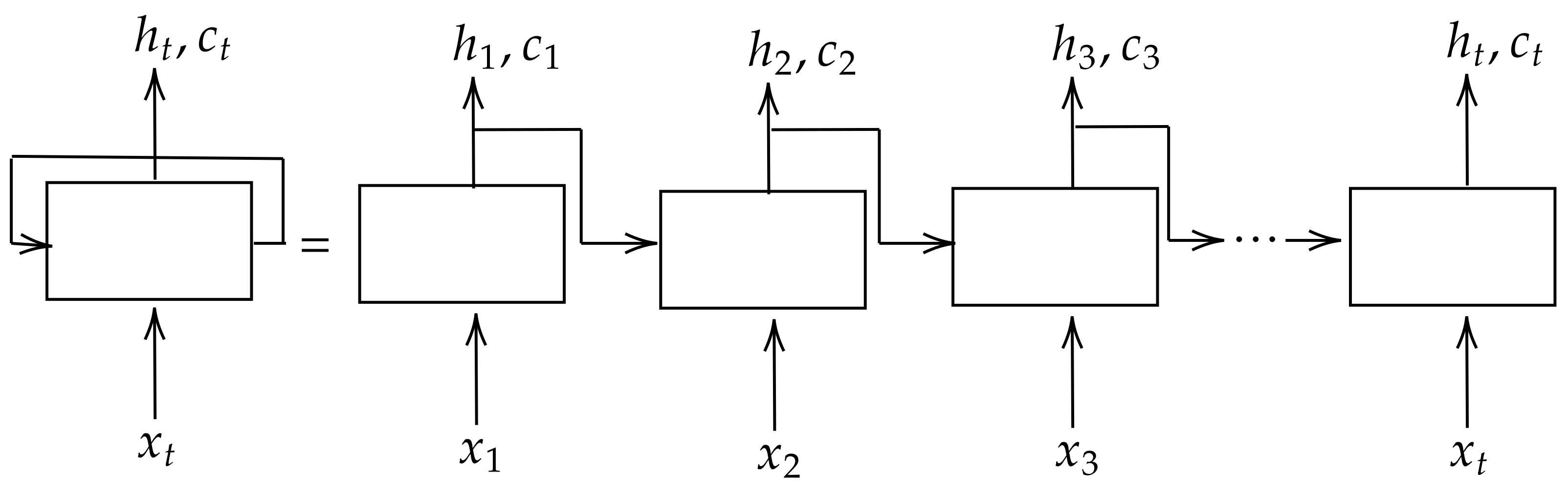
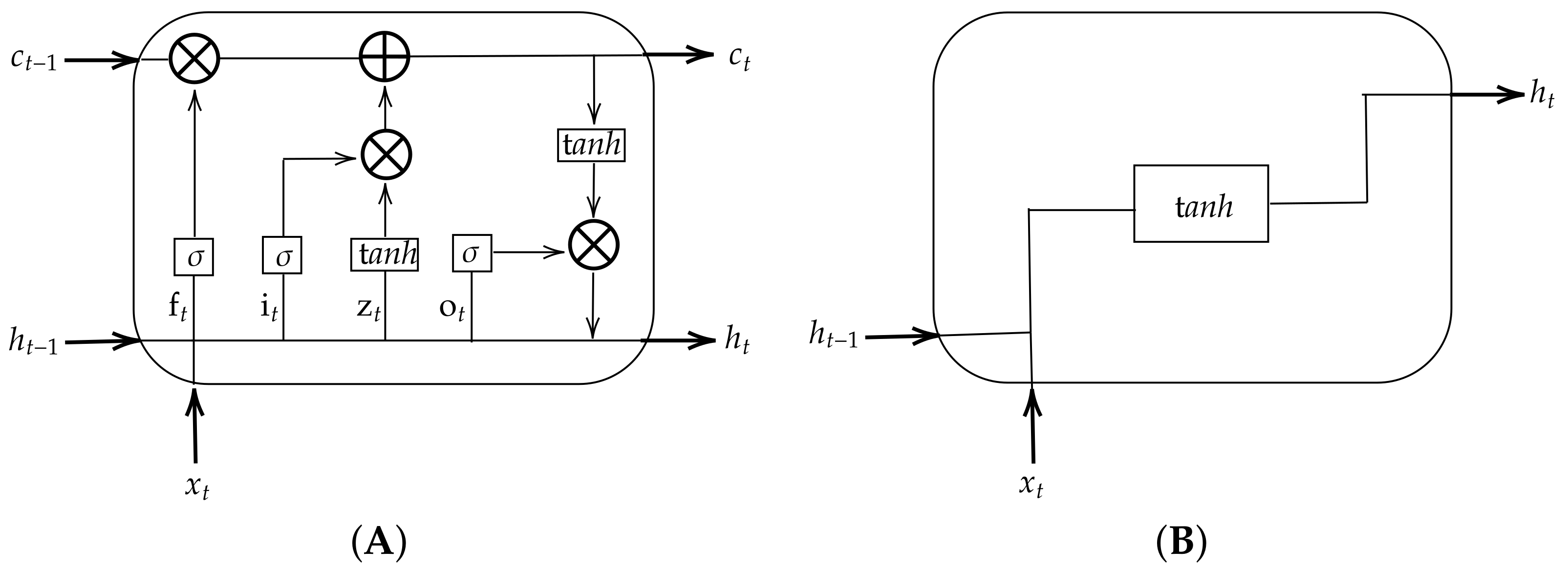
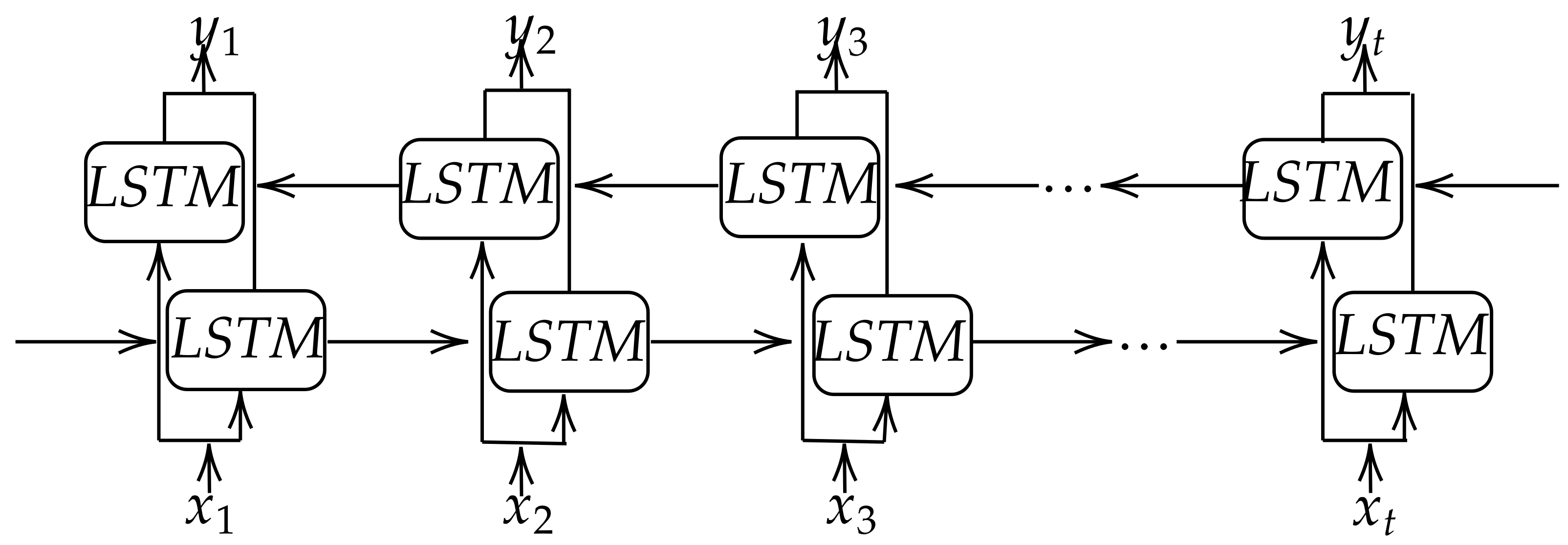
However, traditional machine learning cannot store and learn from the past observations of a time series. Under deep learning, LSTM models are designed to model time series data. Adeyemi et al. [11] developed a Neural Network approach to model temporal soil moisture. In the model evaluation, a value of $R^2$ above 0.94 was obtained at all test sites. Zhang et al. [19] used an LSTM model to predict agricultural water table elevation. They used 14 years of time-series data such as water diversion, precipitation, reference evapotranspiration, temperature, and water table depth. The proposed model achieved higher values of $R^2$ than the model Feed-Forward Neural Network (FFNN) in predicting water table depth. As indicated earlier, measuring reference evapotranspiration volume and soil water volume is time and labor-intensive.

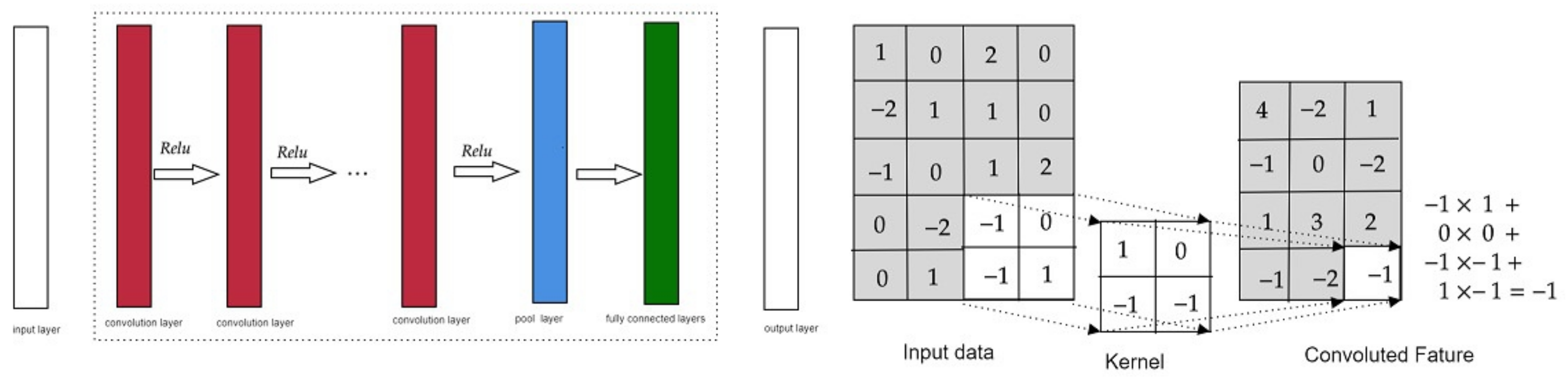
In this paper, a Long Short-Term Memory (LSTM) was developed to predict these two critical parameters. The model forecasts one day- ahead ET and SWC using eight days of historical data. The various evaluation metrics such as Mean Square Error (MSE), Root Mean Square Error (RMSE), Mean Absolute Error (MAE), Mean Bias Error (MBE), and $R^2$ were used to demonstrate the effectiveness of the models. Each metric has its advantages and disadvantages, and as the results of this paper will show, using only one metric can lead to misleading results. The Convolutional Neural Network (CNN) is capable of extracting features from raw data [20]. A CNN model is superimposed on the LSTM model to investigate the performance of CNN- LSTM models compared to LSTM. The performance of the model is also compared with CNN and traditional machine learning algorithms such as Support Vector Regression (SVR) and Random Forest [21,22]. Finally, the impact of the loss function on the training of the model is investigated. The most commonly used loss functions for regression problems are selected, including MSE, RMSE, MAE, and the Huber function. The Huber function is basically MAE, which becomes MSE when the error is small. Unlike MAE, the Huber function is differentiable at 0 and is less sensitive to outliers in the data than MSE [23]. Each of these functions yields a different error for the same prediction and affects the performance of the model on the test set.

2. Materials and Methods

2.1. Data Collection

Data for three sites in Portugal, collected over a period of 7 to 10 years, were used for the training. Datasets were retrieved from the stations Estação Póvoa de Atalaia, Estação Borralheira and Direção Regional de Agricultura e Pescas do Centro, Portugal.

Table 1. Details of the locations in the datasets.

Location	Póvoa de Atalaia (Loc. 1)	Borralheira (Loc. 2)	Fadagosa (Loc. 3)
Longitude	${40}^{°}{4}^{\prime }{15.43}^{″}$ N	${40}^{°}{19}^{\prime }{14.14}^{″}$ N	${40}^{°}{1}^{\prime }{46.55}^{″}$ N
Latitude	$7^{°}{24}^{\prime }{26.02}^{″}$ W	$7^{°}{25}^{\prime }{23.67}^{″}$ W	$7^{°}{26}^{\prime }{36.27}^{″}$ W
Start date	19 September 2013	19 September 2013	16 May 2020
End date	16 May 2020	07 January 2010	23 March 2020
Temporal resolution	daily	daily	15 min

shows details of these sites. The soils of Loc. 1 ana Loc. 3 are of light texture (sandy) or more often of medium texture (sandy loam), permeable, with low to medium organic matter content, with low acid to neutral reaction, rich in phosphorus and potassium, and without salt effects. Climatically, these are areas with mild winters, with precipitation falling mostly in autumn and winter and occasionally in the spring. Usually, temperatures increase significantly from May onwards, peaking in July and occasionally in August, with the registration of several days of maximum temperatures above 40 ${}^{°}$C being common. It has also been noted that registered temperatures reach progressively higher values in September, extending the summer period into October. In the Loc. 2, soils are similar, although soils with medium texture (loam) are more common. Climatically, the regions differ mainly in spring and summer with lower temperature values and higher relative humidity. In terms of precipitation, the values are always higher, and the number of days recorded with precipitation is higher. These plots are covered with fruit trees such as pears, nectarines, cherry, and peach trees.

Datasets Loc. 1 and Loc. 2 were recorded daily, and the Loc. 3 record was recorded every 15 min. These datasets included minimum, maximum, and average temperature; minimum, maximum, and average relative humidity; average solar radiation; minimum and average wind speed; and precipitation.

Table A1. Dataset details.

Variables	Unit	Data Source	Locations	Temporal Resolution	Max	Min	Mean	SD
$T_{Min}$	°C	AppiZezere,	Loc. 1	daily	26.76	−5.26	9.14	5.86
		DRAP-Centro	Loc. 2	daily	21.89	−7.43	7.30	5.39
			Loc. 3	15-min	27	−4.7	9.76	5.63
$T_{Avg}$	°C	AppiZezere,	Loc. 1	daily	35.94	1.96	16.13	7
		DRAP-Centro	Loc. 2	daily	32.2	0	14.66	6.65
			Loc. 3	15-min	34.84	−0.12	15.68	6.90
$T_{Max}$	°C	AppiZezere,	Loc. 1	daily	44.8	5.56	23.97	8.68
		DRAP-Centro	Loc. 2	daily	42.9	4.43	22.99	8.42
			Loc. 3	15-min	42.7	1.8	21.84	8.42
$H{R}_{Min}$	%	AppiZezere,	Loc. 1	daily	99.1	0	41.91	20.56
		DRAP-Centro	Loc. 2	daily	99.1	0	42.78	20.17
			Loc. 3	15-min	95	0	38.72	20.20
$H{R}_{Avg}$	%	AppiZezere,	Loc. 1	daily	99.1	21.84	67.16	18.45
		DRAP-Centro	Loc. 2	daily	99.1	0	70.96	16.34
			Loc. 3	15-min	95.89	27.75	60.38	18.78
$H{R}_{Max}$	%	AppiZezere,	Loc. 1	daily	100	33.33	89.55	13.87
		DRAP-Centro	Loc. 2	daily	99.1	48.37	93.93	10.08
			Loc. 3	15-min	97	24	81.29	15.05
$S{R}_{Avg}$	Wm${}^{-2}$	AppiZezere,	Loc. 1	daily	592.08	3.90	214.67	140.11
		DRAP-Centro	Loc. 2	daily	592.08	3.91	215.57	140.87
			Loc. 3	15-min	346.66	6.35	172.02	89.25
$W{S}_{Avg}$	ms${}^{-1}$	AppiZezere,	Loc. 1	daily	7.28	0.014	1.32	0.81
		DRAP-Centro	Loc. 2	daily	5.91	0	1.06	0.82
			Loc. 3	15-min	28.85	0.031	4.62	3.80
$W{S}_{Max}$	ms ${}^{-1}$	AppiZezere,	Loc. 1	daily	74.04	1.06	4.82	2.16
		DRAP-Centro	Loc. 2	daily	14.65	0	4.87	1.92
			Loc. 3	15-min	86.5	3.5	24.67	10.61
$Prec$	mm d${}^{-1}$	AppiZezere,	Loc. 1	daily	101.59	0	2	6.84
		DRAP-Centro	Loc. 2	daily	112.80	0	2.92	8.95
			Loc. 3	15-min	101.6	0	2.28	7.20
$ETo$	mm d${}^{-1}$	Penman-Monteith	Loc. 1	daily	8.5	0.3	3.260	2.09
		equation	Loc. 2	daily	7.4	0.3	2.83	1.964
			Loc. 3	daily	9.8	0.2	3.68	2.088
$SWC{l}_1$	m${}^3$m${}^{-3}$		Loc. 1	daily at 23:00	0.43	0.097	0.26	0.11
		ECMWF	Loc. 2	daily at 23:00	0.43	0.07	0.27	0.11
			Loc. 3	daily at 23:00	0.43	0.11	0.26	0.10
$SWC{l}_2$	m${}^3$m${}^{-3}$		Loc. 1	daily at 23:00	0.43	0.15	0.28	0.086
		ECMWF	Loc. 2	daily at 23:00	0.43	0.15	0.29	0.08
			Loc. 3	daily at 23:00	0.43	0.15	0.27	0.086
$SWC{l}_3$	m${}^3$m${}^{-3}$		Loc. 1	daily at 23:00	0.43	0.18	0.29	0.06
		ECMWF	Loc. 2	daily at 23:00	0.42	0.2	0.30	0.061
			Loc. 3	daily at 23:00	0.43	0.17	0.28	0.064
$SWC{l}_4$	m${}^3$m${}^{-3}$		Loc. 1	daily at 23:00	0.41	0.27	0.32	0.02
		ECMWF	Loc. 2	daily at 23:00	0.41	0.29	0.33	0.03
			Loc. 3	daily at 23:00	0.4	0.24	0.30	0.037

Abbreviations represent the following: Max: maximum, Min: minimum, SD: standard deviation, Avg: Averag, T: Temperature, HR: relative Humidity, SR: Solar Radiation, WS: Wind Speed, Prec: Precipitation, SWCL_i: Volumetric Soil Water Level i (i ϵ {1,2,3,4}).

in the Appendix A shows the details of these variables. Figure 1 shows the amount of precipitation at each site, which translates to the soil water content in the surface layer of the soil.

The ETo calculator is software developed by the Land and Water Division. The ETo calculator estimates ETo from meteorological data using FAO Penman–Monteith equation [6]. This calculator was used to calculate the daily ETo at these three locations. The amount of soil water content at the end of the day was collected from the ECMWF dataset (ERA5) [24]. ERA5-Land is a reanalysis dataset that provides a consistent view of the evolution of land variables over several decades with improved resolution compared to ERA5. ERA5-Land was created by reproducing the land component of the ECMWF ERA5 climate reanalysis. In particular, ERA5-land runs at a higher resolution (9 km compared to 31 km in ERA5). The reanalysis combines model data with observations from around the world to produce a globally complete and consistent dataset using the laws of physics. The temporal frequency of the output is hourly. ERA5-Land is generated in a single simulation without coupling to the atmospheric module of ECMWF Integrated Forecasting System (IFS) or to the ocean wave model of IFS. It runs without data assimilation, making it computationally affordable for relatively rapid updates. The core of ERA5-Land is the Tiled ECMWF Scheme for Surface Exchanges over Land, which incorporates land surface hydrology (H- TESSEL). It uses the CY45R1 version of the IFS [25].

Soil moisture values refer to the top 7 cm of soil as modeled using the Hydrology Tiled ECMWF Scheme for Surface Exchanges over Land (H-TESSEL) [26] using Richard’s equation for water flow through the unsaturated soil profile [27]. H-TESSEL uses a variety of soil texture classes with specific properties, such as infiltration capacity and wilting point. H-TESSEL has a four-layer representation of the soil (0–7 cm, 7–28 cm, 28–100 cm, 100–289 cm). The volumetric soil water is associated with soil texture, soil depth, and underlying water table [24]. Since layer four is very deep and its role in agriculture applications is limited, layer four was discarded from the dataset, and the three layers between 0 and 100 cm were considered in this study.

Figure 2 shows ETo and SWC at different levels for each site.

2.2. Data Preprocessing

If there are values in the dataset that are missing, invalid, or difficult to process, the algorithm may end up with overfitted, less accurate, or even misleading results. So, before a model can be trained, data preparation procedures such as data transformation, statistical testing, and more must be performed. The missing data were filled in using the moving average method [28].

The other preprocessing in this work involves the removal of collinear parameters and normalization. The collinear parameters contain the same information about the variables and can lead to redundancies in the calculations. For each parameter x and y, the collinear coefficient is calculated by Equation (1) [29]:

$${\rho }_{x,y}=\frac{cov(x,y)}{{\sigma }_x{\sigma }_y}$$

(1)

where $cov(x,y)$, ${\sigma }_x$, and ${\sigma }_y$ are the covariance of x and y, the variance of x, and the variance of y, respectively. The values 1 and −1 of the correlation coefficient indicate the linear and inverse linear correlation, respectively, and the value 0 means no correlation. In this work, if ${\rho }_{x,y}$ exceeded a threshold, then one of the parameters was removed from the dataset. In the end, the parameters temperature ($T_{min}$, $T_{max}$), average humidity ($H{R}_{Avg}$), average wind speed ($W{S}_{Avg}$) and solar radiation ($S{R}_{Avg}$), precipitation ($Prec$), ETo, and SWC were used as inputs to the models.

Table A2. Collinear coefficient between parameters in dataset (Loc. 1 and Loc. 2).

Variables	${\mathbf{T}}_{\mathbf{Min}}$	${\mathbf{T}}_{\mathbf{Avg}}$	${\mathbf{T}}_{\mathbf{Max}}$	${\mathbf{HR}}_{\mathbf{Min}}$	${\mathbf{HR}}_{\mathbf{Avg}}$	${\mathbf{HR}}_{\mathbf{Max}}$	${\mathbf{SR}}_{\mathbf{Avg}}$	${\mathbf{WS}}_{\mathbf{Avg}}$	${\mathbf{WS}}_{\mathbf{Max}}$	$\mathbf{Prec}$	$\mathbf{ETo}$	${\mathbf{SWCl}}_1$	${\mathbf{SWCl}}_2$	${\mathbf{SWCl}}_3$
	Loc. 1
$T_{Min}$	1	0.93	0.82	−0.44	−0.56	−0.56	0.24	0.01	−0.02	−0.04	0.77	−0.66	−0.64	−0.56
$T_{Avg}$	0.93	1	0.97	−0.66	−0.72	−0.58	0.37	−0.11	−0.09	−0.18	0.82	−0.82	−0.78	−0.63
$T_{Max}$	0.82	0.97	1	−0.78	−0.77	−0.56	0.40	−0.20	−0.15	−0.27	0.89	−0.86	−0.81	−0.64
$H{R}_{Min}$	−0.44	−0.66	−0.78	1	0.91	0.62	−0.45	−0.01	0.03	0.46	−0.75	0.79	0.73	0.50
$H{R}_{Avg}$	−0.56	−0.72	−0.77	0.91	1	0.84	−0.41	−0.15	−0.04	-79	−0.79	0.81	0.73	0.51
$H{R}_{Max}$	−0.56	−0.58	−0.56	0.62	0.84	1	−0.22	−0.28	−0.08	0.21	−0.62	0.61	0.54	0.38
$S{R}_{Avg}$	0.24	0.37	0.40	−0.45	−0.41	−0.22	1	0.02	0.10	−0.20	0.027	−0.39	−0.34	−0.17
$W{S}_{Avg}$	0.01	−0.11	−0.20	−0.01	−0.15	−0.28	0.02	1	0.57	0.10	0.069	0.09	0.13	0.18
$W{S}_{Max}$	−0.02	−0.09	−0.15	0.03	−0.04	−0.08	0.10	0.57	1	0.14	−0.007	0.10	0.10	0.12
Prec	−0.04	−0.18	−0.27	0.46	0.37	0.21	−0.20	0.10	0.14	1	−0.24	0.31	0.27	0.13
ETo	0.77	0.89	0.89	−0.75	−0.79	−0.62	0.027	0.069	−0.007	−0.24	1	−0.85	−0.79	−0.57
$SWC{l}_1$	−0.66	−0.82	−0.86	0.79	0.81	0.61	−0.39	0.09	0.10	0.31	−0.85	1	0.95	0.72
$SWC{l}_2$	−0.64	−0.78	−0.81	0.73	0.73	0.54	−0.34	0.13	0.10	0.27	−0.79	0.95	1	0.83
$SWC{l}_3$	−0.56	−0.63	−0.64	0.50	0.51	0.38	−0.17	0.18	0.12	0.13	−0.57	0.72	0.83	1
	Loc. 2
$T_{Min}$	1	0.90	0.73	−0.30	−0.44	−0.39	0.23	0.04	0.05	0.03	0.49	−0.60	−0.60	−0.54
$T_{Avg}$	0.90	1	0.94	−0.60	−0.66	−0.43	0.37	−0.08	−0.04	−0.17	0.60	−0.81	−0.77	−0.63
$T_{Max}$	0.73	0.94	1	−0.76	−0.72	−0.40	0.39	−0.20	−0.16	−0.30	0.58	−0.86	−0.81	−0.63
$H{R}_{Min}$	−0.30	−0.60	−0.76	1	0.88	0.49	−0.42	−0.04	−0.02	0.50	−0.47	0.75	0.68	0.45
$H{R}_{Avg}$	−0.44	−0.66	−0.72	0.88	1	0.75	−0.43	−0.23	−0.15	0.40	−0.44	0.78	0.70	0.47
$H{R}_{Max}$	−0.39	−0.43	−0.40	0.49	0.75	1	−0.17	−0.34	−0.15	0.19	−0.18	0.51	0.45	0.32
$S{R}_{Avg}$	0.23	0.37	0.39	−0.42	−0.43	−0.17	1	−0.0006	0.13	−0.19	0.45	−0.35	−0.30	−0.12
$W{S}_{Avg}$	0.04	−0.08	−0.20	−0.04	−0.23	−0.34	−0.001	1	0.78	0.10	−0.001	0.06	0.10	0.13
$W{S}_{Max}$	0.05	−0.04	−0.16	−0.02	−0.15	−0.15	0.13	0.78	1	0.19	−0.01	0.09	0.11	0.13
Prec	0.03	−0.17	−0.30	0.50	0.40	0.19	−0.19	0.10	0.19	1	−0.16	0.34	0.30	0.16
ETo	0.49	0.60	0.58	−0.47	−0.44	−0.18	0.45	−0.0006	−0.01	−0.16	1	−0.46	−0.38	−0.17
$SWC{l}_1$	−0.60	−0.81	−0.86	0.75	0.78	0.51	−0.35	0.06	0.09	0.34	−0.46	1	0.95	0.74
$SWC{l}_2$	−0.60	−0.77	−0.81	0.68	0.70	0.45	−0.30	0.10	0.11	0.30	−0.38	0.95	1	0.85
$SWC{l}_3$	−0.54	−0.63	−0.63	0.45	0.47	0.32	−0.12	0.13	0.13	0.16	−0.17	0.74	0.85	1

and

Table A3. Collinear coefficient between parameters in dataset (Loc. 3).

Variables	${\mathbf{T}}_{\mathbf{Min}}$	${\mathbf{T}}_{\mathbf{Avg}}$	${\mathbf{T}}_{\mathbf{Max}}$	${\mathbf{HR}}_{\mathbf{Min}}$	${\mathbf{HR}}_{\mathbf{Avg}}$	${\mathbf{HR}}_{\mathbf{Max}}$	${\mathbf{SR}}_{\mathbf{Avg}}$	${\mathbf{WS}}_{\mathbf{Avg}}$	${\mathbf{WS}}_{\mathbf{Max}}$	$\mathbf{Prec}$	$\mathbf{ETo}$	${\mathbf{SWCl}}_1$	${\mathbf{SWCl}}_2$	${\mathbf{SWCl}}_3$
	Loc. 3
$T_{Min}$	1	0.94	0.86	−0.49	−0.55	−0.52	−0.07	0.57	−0.09	−0.08	0.73	−0.66	−0.64	−0.50
$T_{Avg}$	0.94	1	0.98	−0.68	−0.70	−0.56	−0.21	0.74	−0.18	−0.14	0.833	−0.79	−0.74	−0.55
$T_{Max}$	0.86	0.98	1	−0.77	−0.75	−0.56	−0.28	0.79	−0.22	−0.18	0.84	−0.82	−0.77	−0.55
$H{R}_{Min}$	−0.49	−0.68	−0.77	1	0.93	0.68	0.49	−0.81	−0.05	−0.04	−0.77	0.77	0.68	0.42
$H{R}_{Avg}$	−0.55	−0.70	−0.75	0.93	1	0.87	0.44	−0.76	−0.17	−0.12	−0.80	0.77	0.66	0.40
$H{R}_{Max}$	−0.52	−0.56	−0.56	0.68	0.87	1	0.28	−0.51	−0.28	−0.17	−0.67	0.59	70.49	0.31
$S{R}_{Avg}$	0.57	0.74	0.79	−0.81	−0.76	−0.51	−0.40	1	0.02	0.03	0.86	−0.70	−0.60	−0.30
$W{S}_{Avg}$	−0.09	−0.18	−0.22	−0.05	−0.17	−0.28	0.05	0.02	1	0.85	0.121	0.11	0.13	0.18
$W{S}_{Max}$	−0.08	−0.14	−0.18	−0.04	−0.12	−0.17	0.12	0.03	0.85	1	0.118	0.08	0.09	0.12
Prec	−0.07	−0.21	−0.28	0.49	0.44	0.28	1	−0.40	0.05	0.12	−0.284	0.35	0.25	0.09
ETo	0.73	0.833	0.84	−0.77	−0.80	−0.67	0.86	0.121	0.118	−0.284	1	−0.79	−0.70	−0.40
$SWC{l}_1$	−0.66	−0.79	−0.82	0.77	0.77	0.59	0.35	−0.70	0.11	0.08	−0.79	1	0.95	0.68
$SWC{l}_2$	−0.64	−0.74	−0.77	0.68	0.66	0.49	0.25	−0.60	0.13	0.09	−0.70	0.95	1	0.79
$SWC{l}_3$	−0.50	−0.55	−0.55	0.42	0.40	0.31	0.09	−0.30	0.18	0.12	−0.40	0.68	0.79	1
$SWC{l}_4$	0.03	0.04	0.03	−0.05	−0.05	−0.03	−0.02	0.23	0.10	0.06	0.154	0.06	0.15	0.431

in the Appendix A show the collinear coefficients between variables in the different datasets.

The goal of normalization is to bring the values of the dataset to a common scale without distorting the differences in the ranges of values. The standardization formula given by Equation (2) was used to normalize the data [30]:

$$x_{new}=\frac{x_{old}-\overline{x}}{\sigma }$$

(2)

where $\overline{x}$ is the mean value of the data.

2.3. Deep Learning Methods

The LSTM, Bidirectional LSTM, and CNN-LSTM models were used in this paper.

2.3.1. LSTM Architectures

Recurrent Neural Networks (RNN) are specifically designed for processing sequential data. In the RNN model, the output of the previous step is fed into the current step as input. Mathematically, an RNN model is a nonlinear function that takes t-steps of variables in a time series as input and outputs a vector value at time $t+1$ [31]. The output of an RNN unit is determined using a $\tanh$ function by Equation (3):

$$h_t=\tanh (W_x{x}_t+W_h{h}_{t-1}+b_t)$$

(3)

where $h_{t-1}$ is the recurrent output from the previous step, $x_t$ is the input at the current time, and $W_x,W_h,b_t$ are the weights and bias of the network to be trained during the training. The main problem with RNN is the vanishing gradient, i.e., the gradient of the loss function approaches zero [31]. LSTM [32] is a special type of RNN, created as a solution to the vanishing problem in RNN. A single-layer LSTM is shown in Figure 3, where there is one unit for each time step.

A common LSTM unit consists of a block input $z_t$ with corresponding weight matrices $W_{zx},W_{zh},b_z$, an input gate $i_t$ with corresponding weight matrices $W_{ix},W_{ih},b_i$, a forget gate $f_t$ with corresponding weight matrices $W_{fx},W_{fh},b_f$, an output gate $o_t$ with corresponding weight matrices $W_{ox},W_{oh},b_o$, and a memory cell $c_t$ (see Figure 4).

Forget gate $f_t$ determines what information remains in the cell by outputting a number between 0 and 1 using Equation (4). The output 0 means “forget all information completely” and one means “keep all information”. The input gate $i_t$ protects the unit from irrelevant inputs and decides which values to update using Equation (5). The output gate $o_t$ uses the sigmoid function given by Equation (6) to decide which information in the cell is used to calculate the output of the LSTM unit. The block input $z_t$ creates a new vector that could be added to the new state using the $\tanh$ function given by Equation (7). The memory cell $c_t$ decides whether to update the information obtained from the previous inputs and the current information provided by Equation (8).

$$\begin{array}{cc}\hfill f_t& =\sigma (W_{fx}{x}_t+W_{fh}{h}_{t-1}+b_f)\hfill \end{array}$$

(4)

$$\begin{array}{cc}\hfill i_t& =\sigma (W_{ix}{x}_t+W_{ih}{h}_{t-1}+b_i)\hfill \end{array}$$

(5)

$$\begin{array}{cc}\hfill o_t& =\sigma (W_{ox}{x}_t+W_{oh}{h}_{t-1}+b_o)\hfill \end{array}$$

(6)

$$\begin{array}{cc}\hfill z_t& =\tanh (W_{zx}{x}_t+W_{zh}{h}_{t-1}+b_z)\hfill \end{array}$$

(7)

$$\begin{array}{cc}\hfill c_t& =f_t\ast c_{t-1}+i_t\ast z_t\hfill \end{array}$$

(8)

The output of the current block $h_t$ is calculated using Equation (9).

$$h_t=o_t\ast \tanh \left(c_t\right)$$

(9)

2.3.2. Bidirectional LSTM

Bidirectional LSTM (BLSTM) is an extension of the LSTM model that can improve the results [33]. Each layer of a BLSTM is a stack of two LSTM layers, called the forward and backward layers (see Figure 5). The input of the forward layer is the sequence in positive order and computes a sequence of forward hidden states $\overrightarrow{h_1},\dots ,\overrightarrow{h_t}$. The backward layer obtains an inverted copy of the sequence and computes a sequence of the backward hidden states $\overleftarrow{h_1},\dots ,\overleftarrow{h_t}$. The final representation of the observation is obtained by concatenating the forward hidden states with the backward hidden states.

2.3.3. CNN-LSTM Model

CNN is a supervised learning model specifically designed to handle classification, detection, and segmentation [34]. A CNN model consists of a stack of convolutional layers, nonlinear activation functions (e.g., $\tanh$, $\mathrm{ReLU}$), pooling layers (e.g., maximum pooling, average pooling), and fully connected layers [31]. A convolutional layer contains a set of kernels whose parameters must be learned, and it is used to extract features from data. Each kernel slides across the height and width of the input and the dot product between the entries of the kernel, and each position of the input is computed (see Figure 6). A nonlinear activation function is used to introduce nonlinear features into a model. Rectified linear units ($\mathrm{ReLU}$) have become state of the art and are the most commonly used activation function in deep learning models [31]. The output of a $\mathrm{ReLU}$ function is $Max(x,0)$.

A CNN-LSTM model is a participation of the convolutional neural network and an LSTM model. The CNN layers are used to extract features from the input sequence, and an LSTM model is used to support sequence prediction [35].

2.3.4. Dropout

Overfitting occurs when the training loss is small but the generalization of the model to the unseen data is unreliable. To prevent overfitting, it is suggested that regularization techniques such as dropout be used [31]. Dropout is a computationally inexpensive way to regularize during model training by removing units from the network. In LSTM models, dropout can be added to the input layer, outputs, and recurrent outputs [36]. Dropout size is a hyperparameter that should be set during training.

Table 2. Validation MSE for different dropout size (Loc. 3).

	Dropout Size
Dropout on	0.00000	0.10000	0.20000
outputs	0.02050	0.01970	0.01960
inputs	-	0.01996	0.02000
recurrent-outputs	-	0.01950	0.09136

shows the effect of dropout based on the lost validation. In this work, the dropout was used on recurrent outputs.

2.4. Bayesian Optimization

Bayesian optimization is a strategy for the global optimization of black-box functions. A black-box function is an unknown analytic expression of the function, and the evaluation of the function is restricted to a sample at each point [37]. The core components in Bayesian optimization are the objective function, the surrogate model, and the acquisition function. The objective function is the black box function used to maximize compliance with some parameters. For example, in the classification problem, accuracy can be used as the objective function. The surrogate model is a model to approximate the objective function. The Gaussian processes and Parzen-Tree Estimator are the most popular models for the surrogate model [38]. The acquisition function is used to determine where to evaluate the objective function next. There are many options for acquisition functions, such as the Probability of Improvement (PI), Expected Improvement (EI), and upper confidence bound [38].

The Bayesian algorithm is as follows [39]:

• Choose a surrogate function to approximate the objective function and define its prior. The choice of this function is optional; the algorithm is convergent, and the choice of the prior function can help increase the speed of convergence.
• Given a set of observations, Bayes’ rule is used to obtain the posterior distribution over the objective function. Bayes rule is given by Equation (10):

  $$P\left(A\right|B)=\frac{P\left(B\right|A\left)P\right(A)}{P\left(B\right)}$$

  (10)

  where A and B are models and new observations, respectively; $P\left(A\right)$ and $P\left(B\right)$ are the probabilities of the prior distribution (probability that A is true) and the probability that B is observed, respectively; $P\left(A\right|B)$ is the posterior distribution, and $P\left(B\right|A)$ is the likelihood of the event B occurs if model A is true.
• Use an acquisition function $\alpha$ which is a function of the posterior distribution, to determine the next sample point as $x_t=\underset{x}{\mathrm{argmax}}\alpha \left(x\right)$.
• Add the new sample to the observation set and go back to step 2 until convergence or budget has elapsed.

In this paper, Bayesian optimization [40] is used to minimize the loss function in terms of batch size, dropout size, learning rate, and decay. Figure 7 shows the validation loss during Bayesian optimization for Loc. 3.

2.5. Evaluating the Models

Once the model is trained, the critical question is how good the model is. The following metric is used to evaluate the model:

• Mean Square Error (MSE): is the average of the squared differences between prediction and actual observation. In other words, the MSE is the variance of the error [41]. It is calculated by Equation (11):

  $$MSE=\frac{1}{n}\sum _{i=1}^n{(y_i-{\widehat{y}}_i)}^2$$

  (11)
• Root Mean Square Error (RMSE): is the square root of the MSE. In other words, the RMSE is the standard deviation of the error [41]. In the MSE metric, the errors are first squared before averaging, resulting in a high penalty for large errors. Therefore, the RMSE is useful when large errors are undesirable.
• Mean Absolute Error: is the average of the absolute differences between predictions and actual observations and is calculated by Equation (12) [41]:

  $$MAE=\frac{1}{n}\sum _{i=1}^n\left|y_i-{\widehat{y}}_i\right|$$

  (12)
• Mean Bias Error (MBE): captures the average bias in the prediction. A positive bias in a variable means that the data from the datasets are underestimated, while a negative bias means that the model overestimates the observed data. It is calculated by Equation (13):

  $$MBE=\frac{1}{n}\sum _{i=1}^n(y_i-{\widehat{y}}_i)$$

  (13)
• $R^2$: is a statistical measure that calculates the variance explained by the model over the total variance. The higher $R^2$ is, the smaller the differences between the actual observations and the predicted values. It is calculated by Equation (14) [19]:

  $$R^2=1-\frac{{\sum }_{i=1}^n{(y_i-{\widehat{y}}_i)}^2}{{\sum }_{i=1}^n{(y_i-\overline{y})}^2}$$

  (14)

  where $y_i$’s, $y_i$’s, and $\overline{y}$ are the actual observations, the values predicted by the model, and the mean value of the actual observations, respectively.

3. Results and Discussion

The experimental environment configuration consists of an Intel Core i5-4200H CPU, an NVIDIA GEFORCE GTX 950M graphics card, and 6.144 GB RAM. The models were implemented using the Tensorflow framework and the Keras library [42,43].

The dataset was divided into training, validation, and test set (70%, 20%, and 10%, respectively). The model predicted SWC and ETo for one day ahead, considering eight days of historical data, including minimum temperature ($T_{min}$), maximum temperature ($T_{max}$), average humidity ($H{R}_{Avg}$), average wind speed ($W{S}_{Avg}$), and solar radiation ($S{R}_{Avg}$), daily ETo and SWC. Mean square error and Adam optimization method [44] were used for the loss function and optimization method.

Various machine learning algorithms have certain values that should be set before starting the learning process. These values are called hyperparameters and are used to configure the training process. The validation set is used to set the hyperparameters. The hyperparameters of the proposed model are learning rate, batch size, dropout size, number of layers in the model, and number of nodes per layer. The number of hidden layers and the number of nodes per layer were selected manually, and then Bayesian optimization was used to set the remaining hyperparameters. Unlike neural networks, LSTM does not require a deep network to obtain accurate results [20]. Changing the number of nodes per layer has been shown to have a greater impact on results than changing the number of layers [20]. In this work, the number of LSTM layers stayed between 2 and 4 for BLSTM less than 3 and kept the number of nodes per layer below 513. Finally, the network architectures were tested with two, three, and four LSTM layers, with one and two BLSTM layers, and 64, 128, 256, and 512 nodes per layer. The MSE was calculated for the validation dataset with all combinations of the number of layers and the number of nodes, and the results for the different sites are shown in

Table 3. Validation MSE for different number of LSTM layers and LSTM nodes per layer.

Model Architecture	Locations	Number of Nodes per Layer
		64	128	256	512
LSTM-2 layers	Loc. 1	0.01713	0.01197	0.01135	0.01222
	Loc. 2	0.01906	0.01591	0.01446	0.01466
	Loc. 3	0.02064	0.02059	0.02065	0.02035
	Mean	0.018943	0.016156	0.015486	0.015743
LSTM-3 layers	Loc. 1	0.01973	0.01221	0.01114	0.01128
	Loc. 2	0.01923	0.01566	0.01463	0.01460
	Loc. 3	0.02168	0.02089	0.02106	0.02134
	Mean	0.020213	0.016253	0.01561	0.01574
LSTM-4 layers	Loc. 1	0.01911	0.01401	0.01317	0.01156
	Loc. 2	0.02280	0.01623	0.01490	0.01490
	Loc. 3	0.21685	0.15875	0.12353	0.11088
	Mean	0.086253	0.0629	0.05053	0.045886
BLSTM-1 layer	Loc. 1	0.01527	0.01207	0.01104	0.0115
	Loc. 2	0.01870	0.01715	0.01556	0.01522
	Loc. 3	0.02001	0.02023	0.01949	0.01936
	Mean	0.017993	0.016483	0.015363	0.01536
BLSTM-2 layers	Loc. 1	0.01574	0.01374	0.01268	0.01289
	Loc. 2	0.01893	0.01689	0.01583	0.01583
	Loc. 3	0.02017	0.01959	0.01945	0.01982
	Mean	0.01828	0.01674	0.015986	0.01618

. Increasing the number of LSTM layers to four and the number of BLSTM layers to two increased the MSE on the validation dataset, showing the overfitting of the models. Keeping the LSTM layers of two and three for Loc. 1 and Loc. 2 and increasing the number of LSTM nodes per layer, the network accuracy on the validation dataset first increases and then decreases, and the best network accuracy is achieved with 256 nodes. The best accuracy for Loc. 3 was achieved with a single-layer BLSTM with 512 nodes. In the end, the mean error for each architecture was calculated on three datasets, and the single-layer BLSTM with 512 nodes had the best performance with a mean of 0.01536. Among the simple LSTM models, the double-layer LSTM with 256 nodes performed better than the other models.

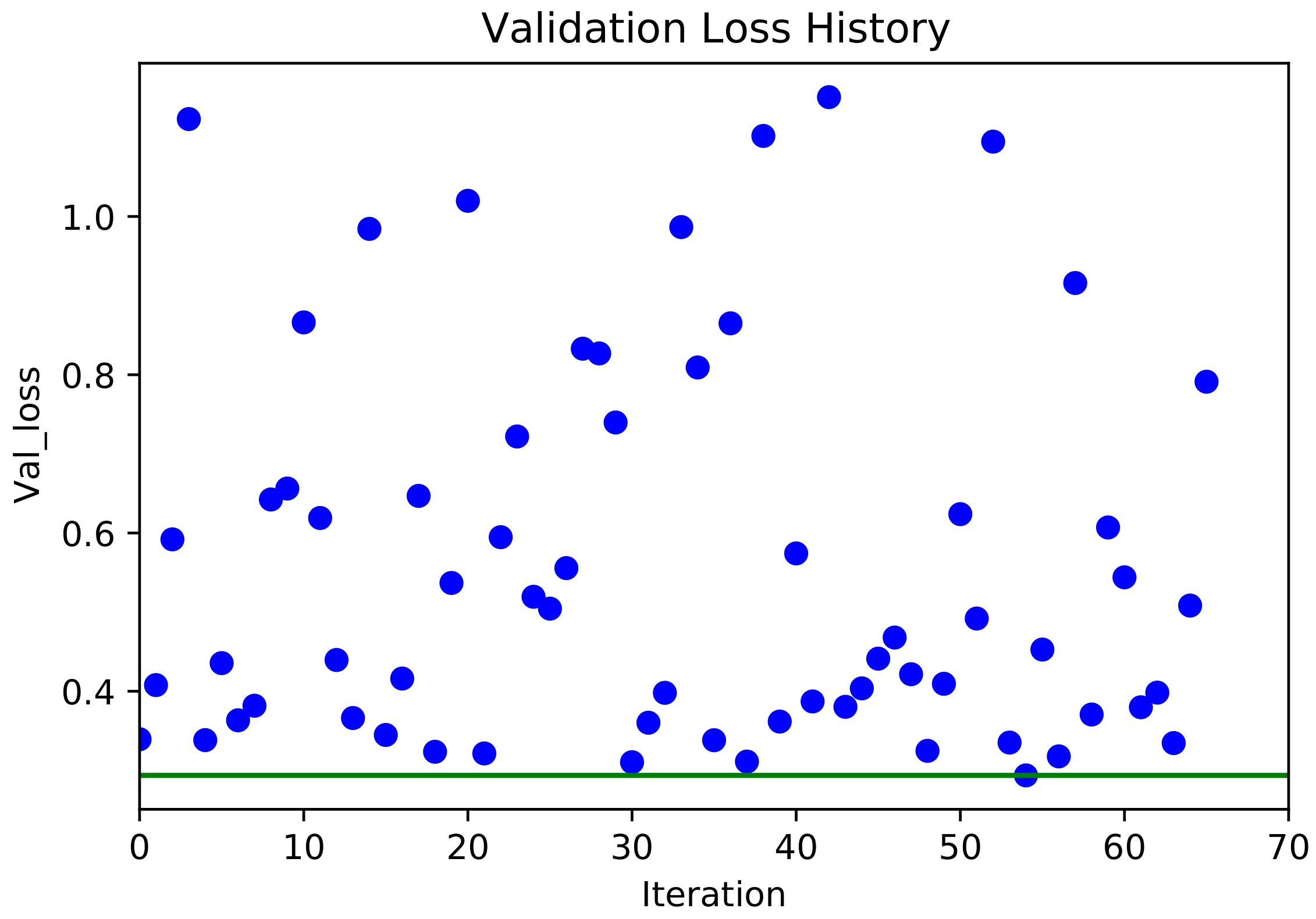
Optimizing the hyperparameters of a machine learning model is simply a minimization problem that seeks the hyperparameters with the least validation loss. Tuning hyperparameters using Bayesian optimization can reduce the time required to find the optimal set of hyperparameters. In this paper, the validation loss in terms of the learning rate, batch size, decay, and dropout size was minimized using Bayesian optimization [40]. Ten steps of random exploration and 60 iterations of Bayesian optimization were performed. Random exploration can help by diversifying the exploration space [40]. The learning rate and decay were kept between ${10}^{-7}$ and ${10}^{-2}$, and the batch size and dropout size were kept in the range of $(32,128)$ and $(0,0.5)$, respectively. For each iteration of the Bayesian optimization algorithm, the network was run for 50 epochs. In the first ten iterations, the algorithm randomly selected the hyperparameters, calculated the validation loss, and then attempted to minimize the validation loss with respect to the hyperparameters (see Figure 7). The validation loss and the selected value for each hyperparameter were stored after each iteration. At the end of 70 iterations, the set of hyperparameters with minimal validation loss was selected. These selected values are shown in

Table 4. Hyperparameters obtained from Bayesian optimization for each location.

Model	Learning Rate	Decay	Batch Size	Dropout Size
BLSTM	${10}^{-4}$	${10}^{-5}$	124	0.2

. For simplicity, the decay and learning rates were modified to a power of 10.

The model was trained on different datasets. Once the model was trained on all datasets (70% of each dataset). The other time, the model was trained on two datasets and tested on the third dataset. Each model was trained for a maximum number of 500 iterations (epoch = 500). Early stopping was used to avoid overfitting. Early stopping is a regularization strategy that determines how many epochs can be run before overfitting begins [31]. In our implementation, the validation error was monitored during training, and if it did not improve after a maximum of ten epochs, training was stopped. 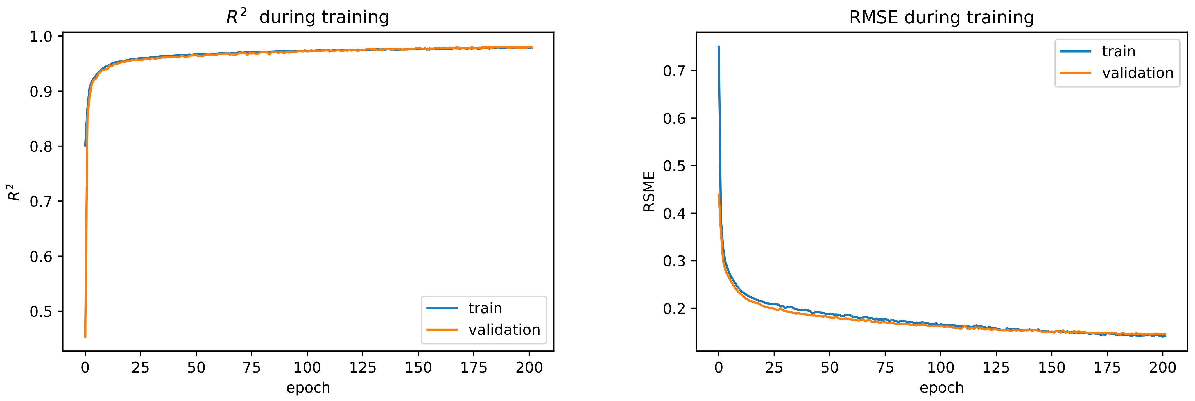Figure 8 shows the $R^2$ and RMSE during training on the training set and the validation set. The error improved after 200 epochs on the training set but did not improve again on the validation set.

Table 5. Evaluation of the LSTM model on the test set for each location. The model was trained on all datasets.

Locations	Metrics	ETo	${\mathbf{SWCl}}_1$	${\mathbf{SWCl}}_2$	${\mathbf{SWCl}}_3$	In-General
Loc. 1	MSE	0.07	0.00074	0.00027	$4.94\times {10}^{-5}$	0.0144
	RMSE	0.29	0.021	0.01	0.004	0.13
	MAE	0.115	0.02	0.013	0.0072	0.12
	$R^2$	0.94	0.9	0.94	0.98	0.98
	MBE	0.032	−0.0013	0.0016	0.003	0.0072
Loc. 2	MSE	0.093	0.0004	$7.48\times {10}^{-5}$	$1.86\times {10}^{-5}$	$0.018$
	RMSE	0.3	0.02	0.0086	0.0043	0.137
	MAE	0.23	0.012	0.005	0.002	0.05
	$R^2$	0.91	0.92	0.98	0.99	0.96
	MBE	−0.024	0.0034	0.0006	0.0004	−0.004
Loc. 3	MSE	0.27	0.0002	$3.8\times {10}^{-5}$	$7.9\times {10}^{-6}$	0.056
	RMSE	0.51	0.016	0.006	0.002	0.23
	MAE	0.36	0.01	0.003	0.0016	0.69
	$R^2$	0.93	0.97	0.99	0.99	0.98
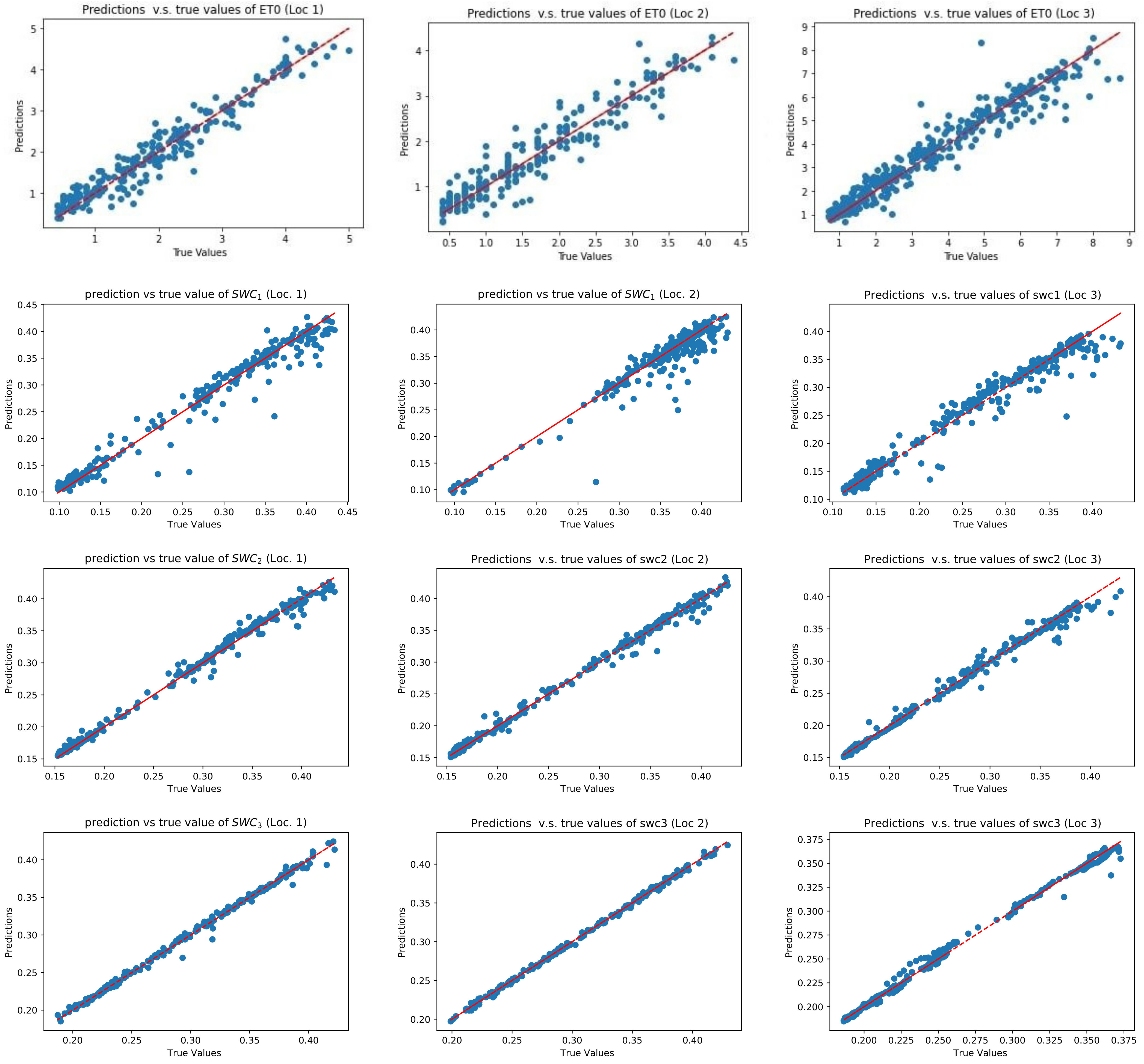
	MBE	−0.06	−0.0007	−0.0007	−0.00027	−0.013

and

Table 6. Evaluation of the LSTM model on the test set for each site. The model was trained on two datasets and tested on the third dataset.

Locations	Metrics	ETo	${\mathbf{SWCl}}_1$	${\mathbf{SWCl}}_2$	${\mathbf{SWCl}}_3$	In-General
Loc. 1	MSE	0.08	0.0004	$9.4\times {10}^{-5}$	$2.3\times {10}^{-5}$	0.016
	RMSE	0.28	0.021	0.009	0.004	0.129
	MAE	0.21	0.013	0.0061	0.0029	0.12
	$R^2$	0.94	0.9	0.94	0.98	0.98
	MBE	0.032	−0.0013	0.0016	0.003	0.0072
Loc. 2	MSE	0.1	0.00047	$7.8\times {10}^{-5}$	$1.89\times {10}^{-5}$	0.02
	RMSE	0.33	0.021	0.0088	0.0043	0.15
	MAE	0.25	0.014	0.006	0.0029	0.055
	$R^2$	0.89	0.91	0.98	0.99	0.95
	MBE	−0.024	0.0034	0.0006	0.0004	−0.004
Loc. 3	MSE	0.35	0.0004	$7.9\times {10}^{-5}$	$1.2\times {10}^{-5}$	0.075
	RMSE	0.59	0.02	0.008	0.003	0.28
	MAE	0.46	0.014	0.005	0.002	0.9
	$R^2$	0.9	0.95	0.98	0.99	0.97
	MBE	−0.26	0.0012	0.0002	0.0005	−0.004

and Figure 9 show the evaluation of the model on the test set and the predicted value compared to the true values of the SWC and ETo, respectively. The results indicated that although the MSE (the variance of the error) at Loc. 2 was lower than the MSE at Loc. 3, the $R^2$- score (the variance explained by the model over the total variance) improved at Loc. 3. Therefore, it is not sufficient to use only one metric to evaluate a model.

As Figure 9 and Table 5 show, the best accuracy in predicting ETo and SWC was achieved with the dataset of Loc. 2 and Loc. 3, respectively. ET was underestimated with the model in Loc. 2 and Loc. 3 but overestimated in Loc. 1. The results also show that as the depth of the soil increases, the accuracy of the model for predicting SWC increases. This could be due to the fact that the range and standard deviation of SWC decrease as the soil depth increases. Adding some other variables to the input of the model, such as irrigation amount, and adding the real data to the simulated dataset may improve the accuracy of the predicted value of SWC in the upper layer (see Table A1).

As the results show, the models trained with two datasets showed similar performance to the model trained with all datasets. The results also show that the model trained with datasets from different locations can be generalized to other locations.

CNN models are capable of extracting features from raw data. The convolutional layers were added to the proposed models to investigate the performance of the CNN- LSTM model for predicting ETo and SWC.

Table 7. CNN used to stake to the LSTM model.

Layer (Type)	Output Shape
Input	(Batch Size, 2, 4, 11)
TimeDistributed(Conv1D)	(Batch Size, 2, 4, N. Filters)
(kernel-size = 3, padding = same)
Dropout 1	(Batch Size, 2, 4, N. Filters)
TimeDistributed(Conv1D)	(Batch Size, 2, 4, N. Filters)
(kernel-size = 2, padding = same)
Dropout 1	(Batch Size, 2, 4, N. Filters)
TimeDistributed(Averagepooling)	(Batch Size, 2, 2, N. Filters)
(pool-size = 2)
TimeDistributed(Flatten)	(Batch Size, 2, $2\times \mathrm{N}.\mathrm{Filters}$)

shows the CNN architectures that were used to stack the LSTM models. First, the input sequence was divided into two subsequences, each with four-time steps. The CNN can interpret each subsequence with four-time steps, and the LSTM used a time series of the interpretations from the subsequences as input. The time-distributed layer wrapped the CNN model and allowed each layer to be applied to each subsequence [43]. The CNN model contained two convolutional layers with kernel sizes of 3 and 2, respectively, followed by an average pooling layer with a pooling size of 2. The number of filters remained the same as the number of nodes in the proposed BLSTM model, i.e., 512 filters in each convolutional layer.

In this paper, the performance of the models was improved by using the function $\tanh$ and the average pooling layer instead of the layer $\mathrm{Relu}$ or Max Pooling (see

Table 8. Performance of the CNN-LSTM model on the test set.

Models	Locations	MSE	RMSE	MAE	${\mathit{R}}^2$	MBE
	Loc. 1	0.161	0.127	0.047	0.974	−0.006
CNN-LSTM	Loc. 2	0.019	0.138	0.051	0.96	−0.003
(AveragePooling+$\tanh$)	Loc. 3	0.063	0.25	0.083	0.976	−0.016
	Loc. 1	0.016	0.12	0.05	0.975	−0.014
CNN-LSTM	Loc. 2	0.021	0.14	0.055	0.95	−0.017
(MaxPooling, $\mathrm{Relu}$)	Loc. 3	0.61	0.24	0.082	0.977	−0.012

).

The performance and computational efficiency of the CNN-BLSTM models are shown in Table 8 and

Table 9. Computation efficiency of the LSTM and CNN-LSTM models.

Models	T(E/S)	N. Param.	N. E	N. P	Tr. S	val. S	Te. S	TT
CNN-LSTM	2	6,842,885	160	20	6197	1550	365	<1 s
LSTM	1	2,151,429	250	20	6197	1550	365	<1 s

Abbreviations represent the following: T: Computational time; E/S: Epoch per second; N.: Number; Param: Parameters; E: Epoch; P: number of patience was used in early stopping method; Tr. S: number of training samples; val. S: number of validation sample; Te. S number of test samples, TT: Computation time for one round of prediction.

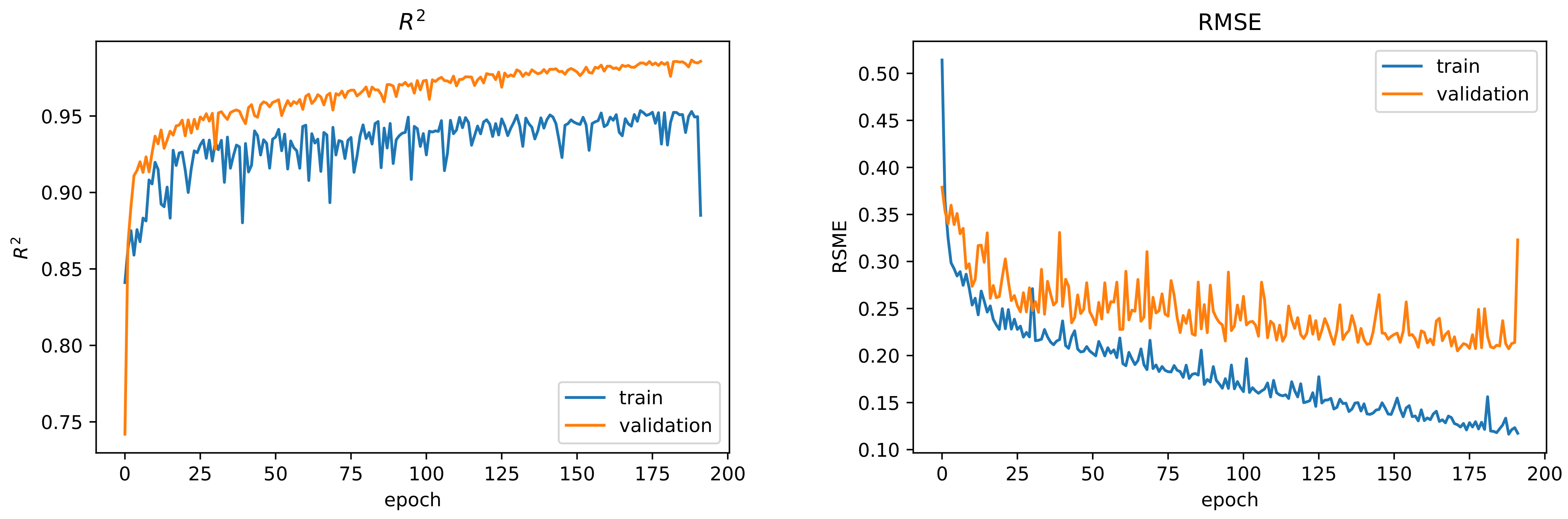
. The BLSTM model outperformed the CNN-BLSTM model in terms of model performance and computation time. As shown in Table 9, the number of trainable parameters tripled in the CNN-BLSTM model compared to the BLSTM. Therefore, the model began to overfit due to the complexity of model. Figure 10 shows the $RMSE$ and $R^2$- score during the training of the CNN-LSTM models.

The performance of the LSTM model was compared with the CNN model and two traditional machine learning models: SVR and Random Forest. The CNN architecture used for the comparison was the same as the CNN architecture built on the LSTM architecture, with the expectation that the time-distributed layers were removed and a dense layer was added in place of the LSTM layers to make the prediction (see

Table 10. CNN architecture used to compare to the LSTM model.

Layer (Type)	Output Shape	Param
Input	(Batch size, 8, 11)	0
(Conv1D)(kernel-size = 3)	(Batch size, 6, N. Filters)	17,408
Dropout 1	(Batch size, 6, 512)	0
(Conv1D)(kernel-size = 2)	(Batch size, 5, N. Filters)	524,800
Dropout 1	(Batch size, 5, N. Filters)	0
(Averagepooling)(pool-size = 2)	(Batch size, 2, N. Filters)	0
Flatten	(Batch size, $2\times \mathrm{N}.\mathrm{Filters}$)	0
Dense	(Batch size, N. Filters)	524,800
Dense	(Batch size, 5)	2565

).

RF is one of the most powerful machine learning methods. The Random Forest consists of several Decision Trees. Each individual tree is a very simple model that has branches, nodes where a condition is checked, and if it is satisfied, the flow goes through one branch, otherwise through the other, and always to the next node until the tree is finished [22].

Support Vector Regression (SVR) is a supervised learning algorithm used to predict discrete values. The basic idea behind SVR is to find the best fitting line. In SVR, the best fitting line is the hyperplane that has the maximum number of input points [21]. A kernel in the SVR model is a set of mathematical functions that take data as input and transform it into the desired shape. They are generally used to find a hyperplane in a higher-dimensional space. The most commonly used kernels include Linear, Nonlinear, Polynomial, Radial Base Function (RBF), and Sigmoid. Each of these kernels is used depending on the dataset. In this work, the RBF kernel has been used [45].

Table 11. Performance of the traditional machine learning algorithms and CNN model on the dataset (MSE).

Locations	Metrics	SVR-RBF	RF	CNN
Loc. 1	MSE	0.2	0.085	0.033
	RMSE	0.45	0.29	0.18
	MAE	0.31	0.21	0.7
	$R^2$	0.81	0.92	0.94
	MBE	0.14	0.002	0.03
Loc. 2	MSE	0.17	0.11	0.027
	RMSE	0.42	0.34	0.16
	MAE	0.31	0.26	0.06
	$R^2$	0.83	0.88	0.94
	MBE	0.14	0.02	−0.03
Loc. 3	MSE	0.33	0.32	0.2
	RMSE	0.58	0.56	0.45
	MAE	0.39	0.39	0.16
	$R^2$	0.92	0.92	0.93
	MBE	−0.023	−0.02	−0.016

shows the performance of each model on the test set. As shown, the LSTM models show better performance on the datasets. The CNN model has achieved the second-best performance.

One of the applications of this model is a decision system that decides when and how much to irrigate in order to avoid water waste without compromising productivity. In future work, a reinforcement learning agent can be trained to select the best amount of irrigation. In deep reinforcement learning algorithms, there is an environment that interacts with an agent. During training, the agent chooses an action based on the current state of the environment, and the environment returns the reward and the next state based on the previous state to the agent. The agent tries to choose the action that maximizes the reward [46]. In the agricultural domain, the state of the environment can be defined as the climate data and the water content of the soil and ETo; the action is the amount of irrigation, and the reward is the net yield. An agent can be trained to choose the irrigation amount based on the state of the field, and the SWC and ET prediction model can be used as part of the environment of Deep Reinforcement Learning to calculate the next state of the environment. By using the trained model in this paper, the training of the agent can be end-to-end and does not require manual processing.

In the end, the importance of the loss function to train the LSTM models was investigated for Loc. 3. The model was trained using MSE, RMSE, MAE, and Huber loss function. The Huber loss function ($H_{\delta }$) is the composition of the MAE and MSE and can be calculated by Equation (15):

$$H_{\delta }=\left\{\begin{array}{cc}\frac{1}{2}{(y-\widehat{y})}^2\hfill & \mathrm{if}|y-\widehat{y}|\le \delta \hfill \\ \frac{1}{2}{\delta }^2+\delta |y-\widehat{y}|\hfill & otherwise\hfill \end{array}\right.$$

(15)

where $\delta$ is a hyperparameter that should be set. The Huber function is basically MAE, which becomes MSE when the error is small. Unlike the MAE, the Huber function is differentiable at 0.

Table 12. Performance of the models using different loss functions for Loc. 3.

Loss Functions	Metrics
	MSE	RMSE	MAE	${\mathit{R}}^2$
MSE	0.056	0.23	0.69	0.98
RMSE	0.067	0.25	0.8	0.975
MAE	0.07	0.07	0.27	0.97
$H_{\delta =1}$	0.063	0.25	0.79	0.976
$H_{\delta =0.1}$	0.068	0.26	0.77	0.974
$H_{\delta =0.01}$	0.074	0.27	0.8	0.972
$H_{\delta =0.001}$	0.062	0.27	0.07	0.977
$H_{\delta =0.0001}$	0.09	0.3	0.1	0.965

shows the performance of the model on the validation set using Huber, MAE, RMSE, and MSE as loss function for Loc. 3. The model with MSE as a loss function outperformed the others.

4. Conclusions

The advantage of the recurrent neural network is its ability to process time-series data like agricultural datasets. In this paper, the ability of recurrent neural networks, including LSTM and its extension BLSTM, to model ETo and SWC was investigated. A drawback of deep learning methods is that they require a large amount of data to train. To overcome this problem, the simulated dataset was used for ET and SWC. The BLSTM model outperformed the LSTM model on the validation set, and hence a single layer BLSTM model with 512 nodes was trained. The proposed model achieved MSE in the range of 0.014 to 0.056, and the results show that the BLSTM model has good potential for modeling ETo and SWC. The CNN models are able to extract features from the data. A CNN model was added to the BLSTM model to extract features, and then BLSTM used these features to predict ET and SWC. When a CNN model was added to the LSTM model, and the number of parameters in the CNN-BLSTM was increased by three times, the model began to overfit after 100 epochs, and BLSTM showed better results than the CNN-BLSTM. Therefore, increasing the number of trainable parameters in deep learning algorithms may cause the model to overfit.

The performance of BLSTM was also compared with Random Forest, SVR, and CNN. The best performance was obtained with BLSTM. The second-best performance was obtained with the CNN model. Among the machine learning methods, RF outperformed the SVR model. One disadvantage of BLSTM compared to CNN, SVR, and RF was that the training time of BLSTM was higher than the other models, but when trained, it was more accurate, and the computation time for prediction was almost the same as the other models.

Finally, the importance of choosing a loss function was investigated. The model with MSE as the loss function performed better than the other models with an MSE of 0.056, and the model with $H_{\delta =0.0001}$ as the loss function had the worst performance. These results show that the choice of a loss function depends on the problem and must be chosen carefully.

In future work, the variables such as irrigation amount and groundwater level will be added to the input of the model to make the prediction more accurate. As mentioned earlier, one of the applications of the SWC and ET prediction model is to develop an end-to-end decision support system that automatically decides when and how much to irrigate. Deep reinforcement learning models are used to build such a system. An agent can be trained to select the amount of irrigation based on the condition of the field. Deep reinforcement learning algorithms require an environment that interacts with the agent and tells the agent the next state and reward. The SWC and ET prediction model is used as part of the algorithms’ environment and determines the next state, which is the SWC and ET a day per head.

References

1. World Urbanization Prospects: The 2018 Revision (ST/ESA/SER.A/420); Technical Report; United Nations, Department of Economic and Social Affairs, Population Division: New York, NY, USA, 2019.
2. Sundmaeker, H.; Verdouw, C.N.; Wolfert, J.; Freire, L.P. Internet of Food and Farm 2020. In Digitising the Industry; Vermesan, O., Friess, P., Eds.; River Publishers: Aalborg, Denmark, 2016; pp. 129–150. [Google Scholar]
3. FAO. World Agriculture 2030: Main Findings. 2002. Available online: http://www.fao.org/english/newsroom/news/2002/7833-en.html (accessed on 1 May 2020).
4. Laaboudi, A.; Mouhouche, B.; Draoui, B. Neural network approach to reference evapotranspiration modeling from limited climatic data in arid regions. Int. J. Biometeorol. 2012, 56, 831–841. [Google Scholar] [CrossRef] [Green Version]
5. Achieng, K.O. Modelling of soil moisture retention curve using machine learning techniques: Artificial and deep neural networks vs support vector regression models. Comput. Geosci. 2019, 133, 104320. [Google Scholar] [CrossRef]
6. Allen, R.G.; Pereira, L.S.; Raes, D.; Smith, M. Crop Evapotranspiration—Guidelines for Computing Crop Water Requirements FAO Irrigation and Drainage Paper 56; FAO—Food and Agriculture Organization of the United Nations: Rome, Italy, 1998. [Google Scholar]
7. Jimenez, A.F.; Cardenas, P.F.; Canales, A.; Jimenez, F.; Portacio, A. A survey on intelligent agents and multi-agents for irrigation scheduling. Comput. Electron. Agric. 2020, 176, 105474. [Google Scholar] [CrossRef]
8. Clulow, A.D.; Everson, C.S.; Mengistu, M.G.; Price, J.S.; Nickless, A.; Jewitt, G.P.W. Extending periodic eddy covariance latent heat fluxes through tree sap-flow measurements to estimate long-term total evaporation in a peat swamp forest. Hydrol. Earth Syst. Sci. 2015, 19, 2513–2534. [Google Scholar] [CrossRef] [Green Version]
9. Kumar, M.; Raghuwanshi, N.S.; Singh, R. Artificial neural networks approach in evapotranspiration modeling: A review. Irrig. Sci. 2011, 29, 11–25. [Google Scholar] [CrossRef]
10. Karandish, F.; Šimůnek, J. A comparison of numerical and machine-learning modeling of soil water content with limited input data. J. Hydrol. 2016, 543, 892–909. [Google Scholar] [CrossRef] [Green Version]
11. Adeyemi, O.; Grove, I.; Peets, S.; Domun, Y.; Norton, T. Dynamic Neural Network Modelling of Soil Moisture Content for Predictive Irrigation Scheduling. Sensors 2018, 18, 3408. [Google Scholar] [CrossRef] [Green Version]
12. Yamac, S.S.; Seker, C.; Negis, H. Evaluation of machine learning methods to predict soil moisture constants with different combinations of soil input data for calcareous soils in a semi arid area. Agric. Water Manag. 2020, 234. [Google Scholar] [CrossRef]
13. Fernandez-Lopez, A.; Marin-Sanchez, D.; Garcia-Mateos, G.; Ruiz-Canales, A.; Ferrandez-Villena-Garcia, M.; Molina-Martinez, J.M. A Machine Learning Method to Estimate Reference Evapotranspiration Using Soil Moisture Sensors. Appl. Sci. 2020, 10, 1912. [Google Scholar] [CrossRef] [Green Version]
14. Tseng, D.; Wang, D.; Chen, C.; Miller, L.; Song, W.; Viers, J.; Vougioukas, S.; Carpin, S.; Ojea, J.A.; Goldberg, K. Towards Automating Precision Irrigation: Deep Learning to Infer Local Soil Moisture Conditions from Synthetic Aerial Agricultural Images. In Proceedings of the 2018 IEEE 14th International Conference on Automation Science and Engineering (CASE), Munich, Germany, 20–24 August 2018; pp. 284–291. [Google Scholar]
15. Song, X.; Zhang, G.; Liu, F.; Li, D.; Zhao, Y.; Yang, J. Modeling spatio-temporal distribution of soil moisture by deep learning-based cellular automata model. J. Arid. Land 2016, 8, 734–748. [Google Scholar] [CrossRef] [Green Version]
16. Adamala, S. Temperature based generalized wavelet-neural network models to estimate evapotranspiration in India. Inf. Process. Agric. 2018, 5, 149–155. [Google Scholar] [CrossRef]
17. Saggi, M.K.; Jain, S. Reference evapotranspiration estimation and modeling of the Punjab Northern India using deep learning. Comput. Electron. Agric. 2019, 156, 387–398. [Google Scholar] [CrossRef]
18. De Oliveira e Lucas, P.; Alves, M.A.; de Lima e Silva, P.C.; Guimarães, F.G. Reference evapotranspiration time series forecasting with ensemble of convolutional neural networks. Comput. Electron. Agric. 2020, 177, 105700. [Google Scholar] [CrossRef]
19. Zhang, J.; Zhu, Y.; Zhang, X.; Ye, M.; Yang, J. Developing a Long Short-Term Memory (LSTM) based model for predicting water table depth in agricultural areas. J. Hydrol. 2018, 561, 918–929. [Google Scholar] [CrossRef]
20. Schmidhuber, J. Deep learning in neural networks: An overview. Neural Netw. 2015, 61, 85–117. [Google Scholar] [CrossRef] [Green Version]
21. Drucker, H.; Burges, C.J.C.; Kaufman, L.; Smola, A.; Vapnik, V. Support Vector Regression Machines. In Proceedings of the 9th International Conference on Neural Information Processing Systems, NIPS’96, Denver, CO, USA, 2–5 December 1996; MIT Press: Cambridge, MA, USA, 1996; pp. 155–161. [Google Scholar]
22. Breiman, L. Random Forests. Mach. Learn. 2001, 45, 5–32. [Google Scholar] [CrossRef] [Green Version]
23. Huber, P.J. Robust estimation of a location parameter. Ann. Math. Stat. 1964, 35, 73–101. [Google Scholar] [CrossRef]
24. Muñoz Sabater, J. ERA5-Land hourly data from 1981 to present. Copernicus Climate Change Service (C3S) Climate Data Store (CDS). 2019. Available online: https://cds.climate.copernicus.eu/cdsapp#!/dataset/reanalysis-era5-land?tab=overview (accessed on 15 April 2021).
25. IFS Documentation CY45R1—Part IV: Physical processes. In IFS Documentation CY45R1; Number 4 in IFS Documentation; ECMWF: Reading, UK, 2018. [CrossRef]
26. Balsamo, G.; Albergel, C.; Beljaars, A.; Boussetta, S.; Brun, E.; Cloke, H.; Dee, D.; Dutra, E.; Muñoz Sabater, J.; Pappenberger, F.; et al. ERA-Interim/Land: A global land surface reanalysis data set. Hydrol. Earth Syst. Sci. 2015, 19, 389–407. [Google Scholar] [CrossRef] [Green Version]
27. Richards, L.A. Capillary conduction of liquids through porous mediums. Physics 1931, 1, 318–333. [Google Scholar] [CrossRef]
28. Montgomery, D.C.; Jennings, C.L.; Kulahci, M. Introduction to Time Series Analysis and Forecasting; Wiley Series in Probability and Statistics; Wiley: Hoboken, NJ, USA, 2011. [Google Scholar]
29. Benesty, J.; Chen, J.; Huang, Y.; Cohen, I. Pearson Correlation Coefficient. In Noise Reduction in Speech Processing; Springer: Berlin/Heidelberg, Germany, 2009; pp. 1–4. [Google Scholar]
30. Kreyszig, E.; Kreyszig, H.; Norminton, E.J. Advanced Engineering Mathematics, 10th ed.; Wiley: Hoboken, NJ, USA, 2011. [Google Scholar]
31. Patterson, J.; Gibson, A. Deep Learning: A Practitioner’s Approach; O’Reilly: Beijing, China, 2017. [Google Scholar]
32. Hochreiter, S.; Schmidhuber, J. Long Short-Term Memory. Neural Comput. 1997, 9, 1735–1780. [Google Scholar] [CrossRef]
33. Schuster, M.; Paliwal, K.K. Bidirectional recurrent neural networks. IEEE Trans. Signal Process. 1997, 45, 2673–2681. [Google Scholar] [CrossRef] [Green Version]
34. Sermanet, P.; Eigen, D.; Zhang, X.; Mathieu, M.; Fergus, R.; LeCun, Y. OverFeat: Integrated Recognition, Localization and Detection using Convolutional Networks. arXiv 2013, arXiv:1312.6229. [Google Scholar]
35. Donahue, J.; Hendricks, L.A.; Rohrbach, M.; Venugopalan, S.; Guadarrama, S.; Saenko, K.; Darrell, T. Long-Term Recurrent Convolutional Networks for Visual Recognition and Description. IEEE Trans. Pattern Anal. Mach. Intell. 2017, 39, 677–691. [Google Scholar] [CrossRef]
36. Gal, Y.; Ghahramani, Z. A Theoretically Grounded Application of Dropout in Recurrent Neural Networks. In Proceedings of the 30th International Conference on Neural Information Processing Systems, NIPS’16, Barcelona, Spain, 5–10 December 2016 ; Curran Associates Inc.: Red Hook, NY, USA, 2016; pp. 1027–1035. [Google Scholar]
37. Mockus, J. Bayesian approach to global optimization. In Mathematics and its Applications (Soviet Series); Theory and Applications, with a 5.25-inch IBM PC Floppy Disk; Kluwer Academic Publishers Group: Dordrecht, The Netherlands, 1989; Volume 37, p. xiv+254. [Google Scholar]
38. Bergstra, J.; Bardenet, R.; Bengio, Y.; Kégl, B. Algorithms for Hyper-Parameter Optimization. In Proceedings of the 24th International Conference on Neural Information Processing Systems, NIPS’11, Granada, Spain, 12–14 December 2011; Curran Associates Inc.: Red Hook, NY, USA, 2011; pp. 2546–2554. [Google Scholar]
39. Brochu, E.; Cora, V.M.; de Freitas, N. A Tutorial on Bayesian Optimization of Expensive Cost Functions with Application to Active User Modeling and Hierarchical Reinforcement Learning; Technical Report; University of British Columbia‚ Department of Computer Science: Vancouver, BC, Canada, 2009. [Google Scholar]
40. Nogueira, F. Bayesian Optimization: Open Source Constrained Global Optimization Tool for Python. 2014. Available online: https://github.com/fmfn/BayesianOptimization (accessed on 1 August 2020).
41. Willmott, C.J.; Ackleson, S.G.; Davis, R.E.; Feddema, J.J.; Klink, K.M.; Legates, D.R.; O’Donnell, J.; Rowe, C.M. Statistics for the evaluation and comparison of models. J. Geophys. Res. Ocean. 1985, 90, 8995–9005. [Google Scholar] [CrossRef] [Green Version]
42. Abadi, M.; Agarwal, A.; Barham, P.; Brevdo, E.; Chen, Z.; Citro, C.; Corrado, G.S.; Davis, A.; Dean, J.; Devin, M.; et al. TensorFlow: Large-Scale Machine Learning on Heterogeneous Systems. 2015. Software Available. Available online: tensorflow.org (accessed on 1 April 2020).
43. Chollet, F. Keras. 2015. Available online: https://keras.io (accessed on 1 April 2020).
44. Kingma, D.P.; Ba, J. Adam: A Method for Stochastic Optimization, 2014. In Proceedings of the 3rd International Conference for Learning Representations, San Diego, CA, USA, 7–9 May 2015. arxiv:1412.6980. [Google Scholar]
45. Chang, Y.W.; Hsieh, C.J.; Chang, K.W.; Ringgaard, M.; Lin, C.J. Training and Testing Low-degree Polynomial Data Mappings via Linear SVM. J. Mach. Learn. Res. 2010, 11, 1471–1490. [Google Scholar]
46. Sutton, R.S.; Barto, A.G. Reinforcement Learning: An Introduction, 2nd ed.; The MIT Press: Cambridge, MA, USA, 2018. [Google Scholar]
Figure 1. Precipitation amount for each site.
Applsci 11 05029 g001
Figure 2. ETo and SWC at different levels for each site.
Applsci 11 05029 g002aApplsci 11 05029 g002b
Figure 3. LSTM in loops and unfolded in sequence.
Applsci 11 05029 g003
Figure 4. (A). Diagram of LSTM unit and (B). regular RNN unit. Left side shows LSTM cell, right side shows RNN cell.
Applsci 11 05029 g004
Figure 5. One layer BLSTM model.
Applsci 11 05029 g005
Figure 6. The left-hand side is the general CNN architecture, and the right-hand side is the convolutional operation.
Applsci 11 05029 g006
Figure 7. Validation loss vs. time using Bayesian optimization.
Applsci 11 05029 g007
Figure 8. R 2 and RMSE during training. The left side shows the R 2 -score and the right side shows the RMSE.
Applsci 11 05029 g008
Figure 9. True values vs. Predicted values. The x-axis indicates true values, and the y-axis indicates prediction values by models.
Applsci 11 05029 g009
Figure 10. The RMSE and R 2 -score of CNN-BLSTM model during training. The left side shows the R 2 -score and the right side shows the RMSE.
Applsci 11 05029 g010