Article

Low-Frequency Expansion Approach for Seismic Data Based on Compressed Sensing in Low SNR

1
Key Laboratory of Deep Oil and Gas, Qingdao 266580, China
2
School of Geosciences, China University of Petroleum (East China), Qingdao 266580, China
3
Intelligence and Manufacture College, Qingdao Huanghai University, Qingdao 266427, China
*
Authors to whom correspondence should be addressed.
Appl. Sci. 2021, 11(11), 5028; https://doi.org/10.3390/app11115028
Submission received: 18 April 2021 / Revised: 26 May 2021 / Accepted: 27 May 2021 / Published: 29 May 2021
(This article belongs to the Section Applied Physics General)

Abstract

:

Featured Application

The proposed method can improve the anti-noise-interference ability in the inversion procedure of compressed sensing, improve the low-frequency expansion effect for seismic data with a low SNR and further enhance the accuracy of the subsequent inversion and interpretation work.

Abstract

Low-frequency information can reflect the basic trend of a formation, enhance the accuracy of velocity analysis and improve the imaging accuracy of deep structures in seismic exploration. However, the low-frequency information obtained by the conventional seismic acquisition method is seriously polluted by noise, which will be further lost in processing. Compressed sensing (CS) theory is used to exploit the sparsity of the reflection coefficient in the frequency domain to expand the low-frequency components reasonably, thus improving the data quality. However, the conventional CS method is greatly affected by noise, and the effective expansion of low-frequency information can only be realized in the case of a high signal-to-noise ratio (SNR). In this paper, well information is introduced into the objective function to constrain the inversion process of the estimated reflection coefficient, and then, the low-frequency component of the original data is expanded by extracting the low-frequency information of the reflection coefficient. It has been proved by model tests and actual data processing results that the objective function of estimating the reflection coefficient constrained by well logging data based on CS theory can improve the anti-noise interference ability of the inversion process and expand the low-frequency information well in the case of a low SNR.

1. Introduction

The propagation distance of the low-frequency components in seismic data is much longer than that of the high-frequency components, and the content it carries is more abundant. Due to the slow attenuation of low-frequency information and strong penetrating ability, it can be used to improve the imaging quality of complex structures [1,2]. Seismic exploration on land faces challenges from complex surface conditions, such as severe lateral velocity variation and complex terrain [3]. Deep seismic exploration in this complex situation has higher requirements for low-frequency information. In the full waveform inversion, the frequency information below 10 Hz plays an important role [4]. If the seismic data contain high-fidelity low-frequency information, the accuracy requirements for the initial model will be greatly reduced. Zhang et al. analyzed in detail the impact of missing low-frequency information on the resolution of the profile and waveform inversion [5]. At present, low-frequency information below 10 Hz in seismic data obtained by conventional acquisition methods is severely contaminated by noise, and the effective low-frequency information will be further lost during processing such as surface wave suppression. Therefore, the recovery of low-frequency information has very practical significance for deep seismic exploration.
Deconvolution is an indispensable part of seismic data processing. It compresses the wavelets by eliminating the filtering effect of the earth to obtain the seismic reflection coefficient and ultimately improve the resolution of the data [6,7]. In the 1950s, Silvia and Robinson first proposed a time series convolution model [8], which regarded the seismic trace as a convolution of a white noise reflection sequence and a minimum phase seismic wavelet, and proposed a predictive deconvolution method. Then, Wiggins proposed the minimum entropy deconvolution algorithm by adjusting the inverse wavelet to maximize the output timing variance mode, finally obtaining the reflection coefficient. The algorithm does not need to make any assumptions about the wavelet phase [9]. Claerbout, Gray, Ooe, Godfrey and Walden have successively conducted in-depth research on this method [10,11,12,13,14]. Larue et al. and Bann et al. proposed a deconvolution algorithm based on minimizing the mutual information rate and implemented the deconvolution algorithm in the frequency domain [15,16]. Rosa et al. introduced the spectral simulation algorithm into the deconvolution process, which further improved the resolution of seismic data [17]. In addition, Guan et al. [18] used predictive filtering methods in the frequency domain to extrapolate the frequency spectrum of seismic data and successfully expanded the low-frequency components of the seismic signal. Masoomzadeh et al. [19] and Guo Shuxiang et al. [20], respectively, proposed spatial spectrum whitening and frequency division denoising processing methods, which can effectively protect the low-frequency energy in seismic data. After that, Woodbum et al. [2] used the zero-phase matching operator to perform frequency expansion on the low-frequency part of the zero-phase wavelet to improve the amplitude spectrum of a low frequency signal and realize the expansion for the low-frequency component. Han et al. [21] and Zhang et al. [5] successively proposed a low-frequency expansion method based on the compressive sensing (CS) theory and achieved certain results. However, this method is greatly affected by noise. When the noise interference is weak, the reflection coefficient obtained is more accurate, but when the noise is strong, the accuracy of the obtained reflection coefficient will be greatly reduced.
The collected data from well logs have a very high vertical resolution and are rich in information of different frequency bands. Well logging is a significant tool that assists geophysicists with making constraints, guidance and quantity analysis regarding low resolution seismic data [22]. Zhang et al. proposed an inversion method using logging data to improve the resolution and the signal-to-noise ratio (SNR) of seismic records [23]. Firstly, the initial reflection coefficient model is constructed using logging, seismic and geological information. Then, the reflection coefficient is convoluted with the estimated seismic wavelet to obtain a synthetic seismic record. Finally, the correlation between synthetic records and actual seismic records is analyzed, and the reflection coefficient model is modified repeatedly to maximize the correlation coefficient between synthetic records and actual seismic records, thereby obtaining the optimal reflection coefficient. This method has a relatively large dependence on the accuracy of the initial reflection coefficient model during inversion. If the initial model has a wider frequency band, the final reflection coefficient will be more accurate. Pedersen-Tatalovic et al. proposed a multivariate interpolation method based on logging data to improve the accuracy of low-frequency prediction by estimating the layer velocity, layer depth, and layer thickness of seismic data [24]. This method can significantly improve the wave impedance information above 2–8 Hz. Due to considerations of the geological background, the modeling process of this method is more complicated.
In order to improve the accuracy of low-frequency compensation and avoid the dependence of the well-constrained seismic trace inversion method on the accuracy of the initial model, this paper develops low-frequency protection and frequency expansion processing technology of well-constrained seismic data under the framework of CS and uses the well data to constrain the sparse inversion process so as to realize low-frequency compensation for noisy seismic data.

2. CS Theory

CS theory was proposed by David Donoho and Emmanuel Candès [25,26,27,28]. It is a technique that reconstructs sparse, compressible signals from under-determined random linear measurements [29]. Generally, CS theory consists of a sparse representation, a measurement matrix and a sparse promotion algorithm. The two principles of the theory are the sparsity of the signal and the uncorrelation between the measurement matrix and the sparse transformation matrix.
Assuming that transform domain set Ψ can sparsely represent discrete data dRN, the matrix form is expressed as follows:
d = Ψ T E = j = 1 N e j ψ j T
where Ψ = [Ψ1, …, ΨN]∈RN is the basis function vector in the transform domain, ΨT is the inverse transformation of Ψ, N is the total number of basis functions, vector e = [e1, e2,…,eN], ej = <d, Ψj > (j = 1, …, N) is the coefficients in the sparse domain.
Measurement signal dobsRn can be regarded as complete signal d obtained by mapping the sampling matrix, ΦRn×N:
d o b s = Φ d
where n is the number of the collected data points, n << N, Φ: = RM,M is the measurement matrix and R is the constraint matrix. Substitute Formula (1) into Formula (2):
d o b s = Φ Ψ T E = Θ E
where Θ = [Θ1, …, ΘP] is the model matrix, and Θi: = RMΨiTRn×N. According to the theory of CS, the premise of stably reconstructing the Ki maxima of the ith feature of an N dimensional signal is that Θi needs to satisfy the restricted isometry property (RIP) [30,31]. For a K sparse vector (length is N), if ΘRM×N satisfies the following conditions:
( 1 δ ) e l 2 2 Θ e l 2 2 ( 1 + δ ) e l 2 2
where δ is the RIP constant. Generally, if 0 < δ < 1 is satisfied, it is considered that all submatrices of matrix Θ have at most K columns that satisfy the condition, and Θ satisfies the K-order RIP property with δ. Any matrix can be used as a measurement matrix for data reconstruction as long as it conforms to the RIP properties described in Equation (4) [32,33], which theoretically guarantees that the K sparse signal d can be completely recovered from the measurement signal dobs.
In CS theory, the number of observation signals is much smaller than the length of the signal itself, and the recovery of K sparse signal d by Formula (3) requires solving the underdetermined equations. If the signal d is sparse, the problem of solving underdetermined equations can be transformed into a minimum zero norm problem:
min Ψ T E 0 s . t . A C S E = Φ Ψ E = D
where ACS is the model matrix, which consists of the sampling matrix and sparse transformation matrix.
Combinatorial optimization is an NP problem. When N is very large, it cannot be effectively realized numerically, and the anti-noise ability is very poor. When measurement matrix Φ satisfies RIP, Formula (5) can be transformed into a convex optimization problem that is numerically easy to deal with the l1 constraint:
min Ψ T E 1 s . t . A C S E = Φ Ψ E = D
The method of solving Equation (6) can be roughly divided into three categories: a greedy algorithm, convex optimization algorithm and other algorithms (such as Bayesian class, iterative threshold, minimum total variation and related improved algorithms). The greedy algorithm [34,35,36] selects a local optimal solution in each iteration of the solution process, and finally obtains the global optimal solution. The most important feature of this algorithm is its fast solving speed. The disadvantage of the algorithm is that it requires a great deal of input data, and the accuracy of the optimal solution is low. A convex optimization algorithm [37,38] is a more global optimization to improve the inefficiency in the greedy algorithm. It converts the non-convex optimization problem into a convex optimization problem to calculate the approximate value of the signal and minimizes it under the global criterion. This algorithm has a high calculation accuracy and requires less measurement data. The disadvantage of this algorithm is its slow calculation speed. Iterative threshold technology is often used in sparse optimization algorithms [39,40,41]. For example, when processing high-dimensional data, this technology can reduce the computational complexity and improve computational speed in each iteration.

3. Low Frequency Expansion

The basic idea of the convolution model is as follows: when a seismic wavelet passes through the underground reflection interface, it will produce a reflection wave, which can be superimposed to obtain a seismic record. Figure 1 shows the synthetic seismogram convoluted by seismic wavelet (30 Hz) and seismic reflection coefficients. It can be seen that the seismic reflection coefficients are sparse in time domain, and its spectrum is full bandwidth, while the low-frequency information of synthetic seismic record is missing, which is caused by the filtering effect of seismic wavelet. Due to the time-domain sparsity and the frequency-domain full bandwidth of seismic reflection coefficients, Han et al. [22] and Zhang et al. [5] successively proposed the problem of sparse inversion with structural L1 norm constraints. In the frequency domain, the full-bandwidth spectrum is reconstructed through a limited bandwidth, thereby recovering the full-bandwidth energy to a certain extent.

3.1. Basic Theory

Suppose w is seismic wavelet, r is underground reflection coefficient, g is noisy seismic data, and n is random noise; g can be described as:
g = w r + n
Formula (7) is transformed to the frequency domain by Fourier transform:
G = W R + N = W F r + N
where F is the basis function of Fourier transform. G, W, R and N are sparse representations of g, w, r and n in the frequency domain.
The reflection coefficient r in convolution model is sparse in time domain, which conforms to the precondition of CS theory. According to CS theory, the L1 norm optimization problem for solving the underdetermined linear equation in Equation (8) is as follows:
J = 1 2 W R G 2 2 + λ r 1 1 = 1 2 W F r G 2 2 + λ r 1 1
where 2 2 is the error function of L2 norm constraint; W is the measurement matrix constructed by seismic wavelet w, W i j = w i τ j + 1 , τj represents the reflection coefficient location; F is the sparse representation matrix; 1 1 is the exact solution of L1 norm constraint; λ is a regularization parameter, which is used to adjust the weights of the two norms to ensure the balance between sparsity and data fidelity. The larger the λ is, the larger the weight of the L1 norm is, and the sparser the reflection coefficient is. The first term of Equation (9) is constrained by L2 norm and converges to complete seismic data in the process of solution. The second term of Equation (9) is constrained by the L1 norm to obtain more sparse reflection coefficient r.
Based on the obtained sparse reflection coefficient r ˜ , the full band spectrum R ˜ can be expressed as:
R ˜ = F r ˜
R ˜ is the spectrum of the seismic reflection coefficient in the full-frequency band obtained from limited bandwidth seismic data. Assuming that the original data spectrum is G, the frequency spectrum after compensation is G ˜ . The specific method of using R ˜ to expand the low frequency information in seismic data is as follows:
(1)
Select the point where R ˜ and G are equal;
(2)
The spectrum value in R ˜ before the point and the spectrum value in G after the point are extracted and combined into the spectrum after low-frequency expansion; the formula is described as follows:
G ˜ = L ( R ˜ ) + H ( G )
where L and H are the operators to extract the low-frequency and high-frequency spectrum values, respectively.
(3)
The seismic data after low-frequency expansion can be obtained by inverse Fourier transform of G ˜ .
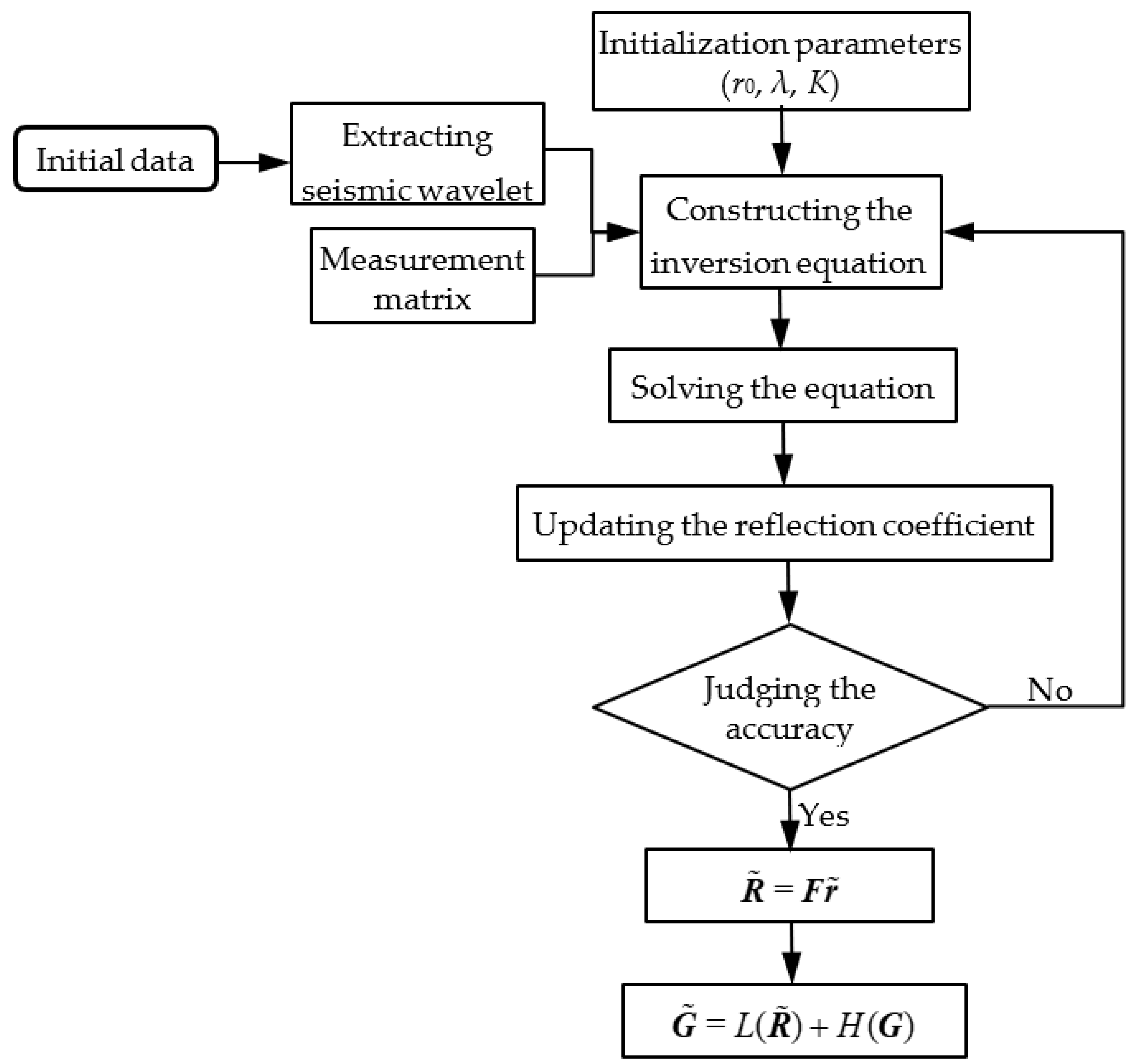
The low-frequency expansion process based on CS is shown in Figure 2.
Note that in Equation (8), the sampling matrix W formed by the Fourier transform of w is not a completely random function, so the missing frequency information of the seismic data is also recovered to a certain extent.

3.2. Well Constrained Low-Frequency Expansion Method

In the framework of CS theory, low-frequency information can be recovered in the frequency domain by using the sparsity of reflection coefficients in the time domain and frequency domain. This method is greatly affected by noise; that is, the reflection coefficient is more accurate when noise is weak. Otherwise, the accuracy of the reflection coefficient will be greatly reduced. In this section, well data are introduced into the cost function to constrain the inversion process so as to improve the accuracy of the reflection coefficient inversion.
For the noisy seismic data G, the cost function with well constraint is constructed as follows:
min r 1 2 G F W r 2 2 + λ r w r ^ w 2 2 s . t . r 1 1 σ
where σ is the noise standard deviation estimation of reflection coefficient, rw is the reflection coefficient at the well location, and r ^ w is the reflection coefficient estimated from the well information.
The cost function can also be solved by a greedy algorithm, base pursuit algorithm or iterative threshold algorithm. The iterative threshold method has a simple structure, less calculation and good stability, so this method is adopted to solve the cost function. The iterative formula is as follows:
r j + 1 = T λ k ( r j + 1 α [ ( W F ) T ( G W F r j ) + λ R w T ( R w r j r ^ w ) ] , λ α )
where WF is the measurement matrix, which is composed of wavelet operator and Fourier transform operator. (WF)T is the conjugate transpose of WF. Rw is the sampling operator to extract the location information of the corresponding well. R w T is the conjugate transpose of Rw.
The reflection coefficient of anti-noise interference can be obtained by iterating Formula (13), and then the expanded seismic data can be obtained according to Equations (10) and (11).

3.3. Algorithm Implementation

In the framework of CS theory, low-frequency information can be recovered in the frequency domain by using the sparsity of reflection coefficients in the time domain and frequency domain. This method is greatly affected by noise; that is, the reflection coefficient is more accurate when noise is weak. Otherwise, the accuracy of reflection coefficient will be greatly reduced. In this section, well data are introduced into the cost function to constrain the inversion process.
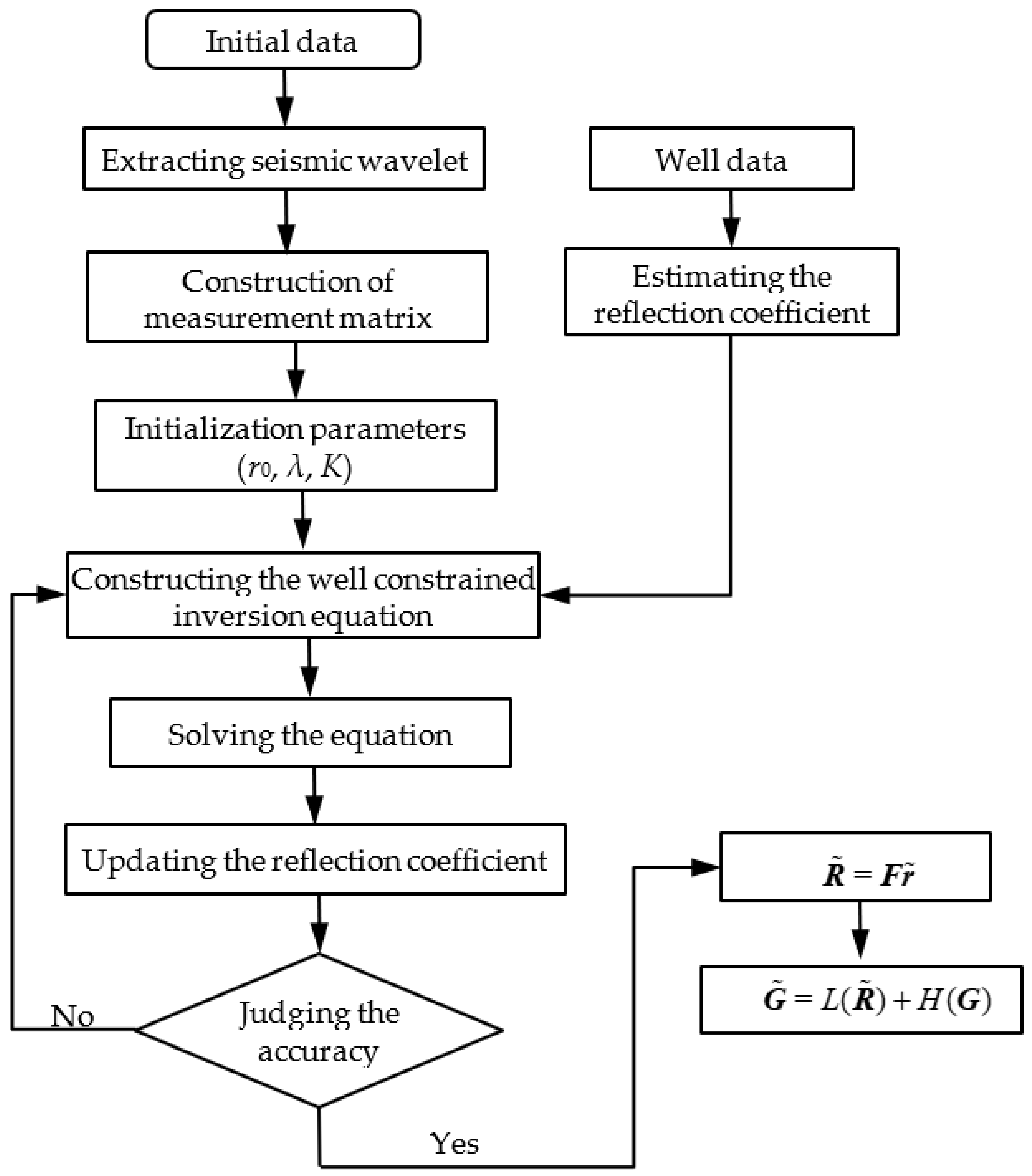
The implementation process of the algorithm after introducing the well data is shown in Figure 3.
Formula (13) is solved by gradient descent algorithm, and the specific implementation algorithm is as follows:
Initializing: ∀r0, Lin (maximum number of iterations in the inner loop), Lout (maximum number of iterations in the outer loop), ε (residual error), k = 1;
Well data processing: the reflection coefficient r ^ w is estimated by well data;
Iteration start:
r0 = r0;
External circulation: judging G W F r k 2 > ε a n d k L o u t
r 0 = r k 1
Internal circulation: j = 0 to Lin-1, r j + 1 = T λ k ( r j + 1 α [ ( W F ) T ( G W F r j ) + λ R w T ( R w r j r ^ w ) ] , λ α ) ;
Implement: k = k + 1; r k = r L i n ;
Calculate the spectrum R ˜ after frequency expansion: R ˜ = F r ˜ ;
Calculate the spectrum G ˜ after frequency expansion: G ˜ = L ( R ˜ ) + H ( G ) ;
Obtain the seismic data after low-frequency expansion: g ˜ = F 1 ( G ˜ ) .
In the above algorithm, T λ is the threshold function; Rw is the sampling operator to extract the location information of the corresponding well; α and λ are the algorithm parameters; α must be greater than the maximum eigenvalue of (WF)TWF; λ adjusts the sparsity of the reflection coefficient; L and H are operators for extracting low-frequency and high-frequency spectrum values, respectively.

4. Application to Seismic Data

4.1. Synthetic Data Example

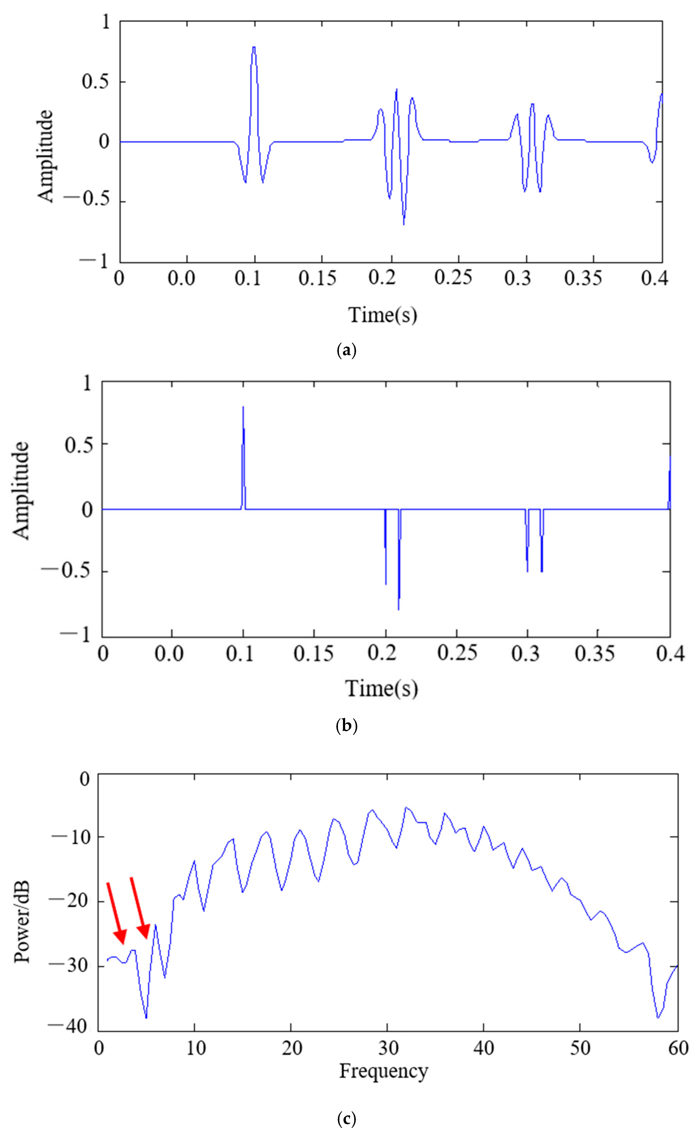
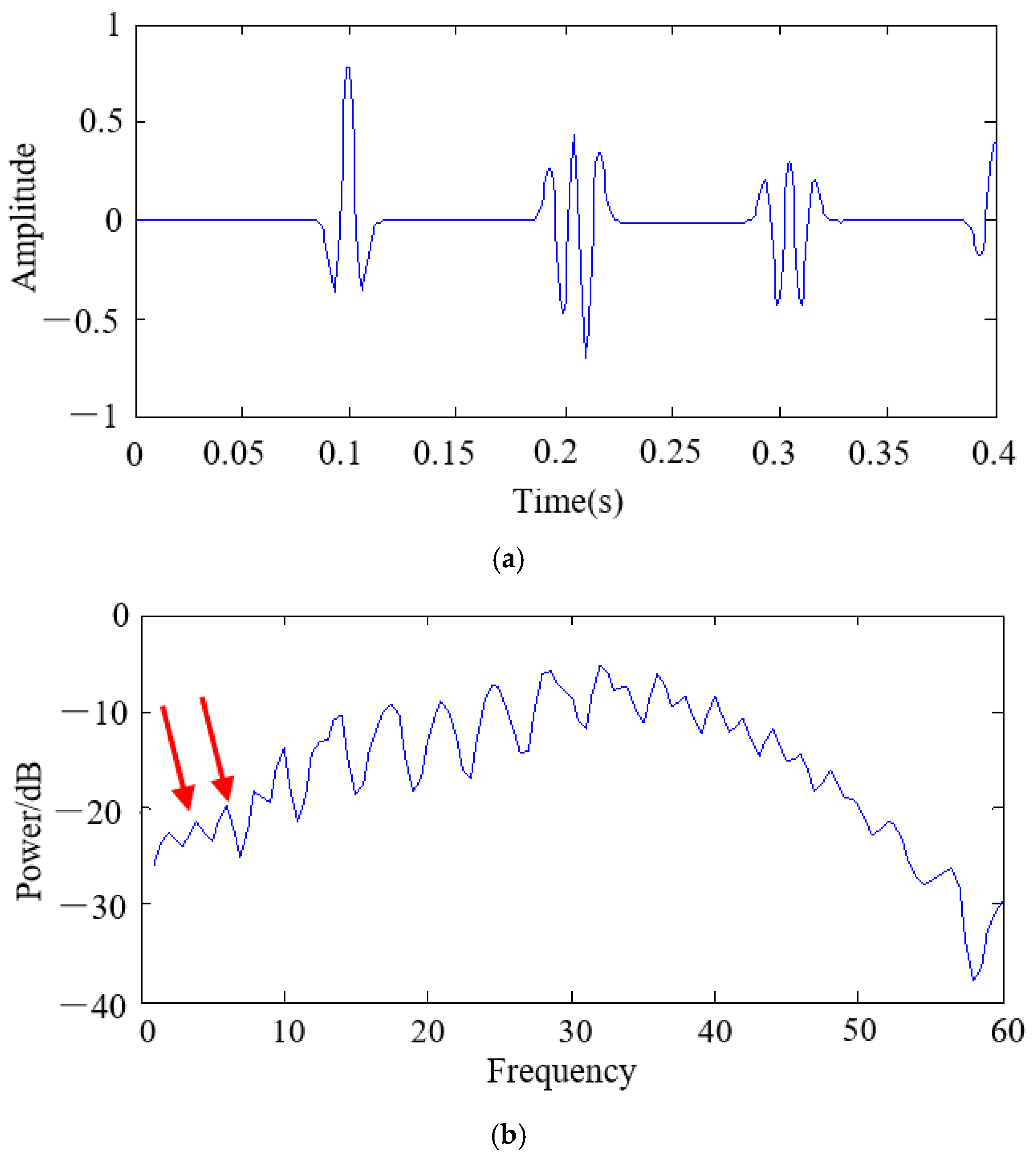
The reflection coefficients at 0.1 s, 0.2 s, 0.21 s, 0.3 s, 0.31 s and 0.4 s are defined as 0.8, 0.6, 0.8, 0.4, 0.4 and 0.4, respectively. The sampling point is 400 and the sampling frequency is 1ms. The synthetic seismogram is obtained by convolution of the reflection coefficient and the Riker wavelet with dominant frequency of 30 Hz, as shown in Figure 4a. The corresponding reflection coefficients and spectrum are shown in Figure 4b,c, respectively. Fourier transform is performed on the composite record to obtain the reflection coefficient of the whole frequency band, and the low-frequency part of the reflection coefficient and the high frequency part of the composite record are taken to form a new spectrum as shown in Figure 5b. Figure 5a is the seismic record after low-frequency expansion. Comparing the results before (Figure 4c) and after frequency expansion (Figure 5b), it can be seen that the low-frequency energy (0–7 Hz) has been significantly improved from −29 dB to −22 dB, especially the energy at 5 Hz is improved obviously. Clearly, the low-frequency expansion method based on the CS theory can extend the low-frequency of the data well.
Different intensity noise is added to the synthetic seismogram to test the anti-noise ability of this method. The noise data with different SNR (14.72, 9.41, 5.10 and 3.14) are shown in Figure 6a, Figure 7a, Figure 8a, Figure 9a. It can be seen that the effective signal is gradually submerged in the noise with the decrease in SNR. For these noisy seismic records, the sparse inversion method based on compressed sensing and the proposed method are used, respectively.
When the SNR of seismic record is 14.72, the reflection coefficients are calculated by the CS method and the well constrained CS method, and then the spectrum of seismic record after frequency expansion is compared. Figure 6a is the noisy seismic record, Figure 6b is the spectrum of the noisy data. Figure 6c,e shows the reflection coefficients obtained by the two methods, respectively. It can be seen that both methods can accurately reverse the reflection coefficient. Comparing the spectrum before (Figure 6b) and after frequency expansion (Figure 6d,f), it can be seen that the low-frequency energy (especially in 0–5 Hz) have been significantly improved from −50 dB to −22 dB. It shows that the low-frequency information has been extended and the frequency band has also been broadened to a certain extent.
The SNR is reduced to 9.41 (Figure 7a), and Figure 7b is its spectrogram. It can be seen that the energy of low-frequency energy in Figure 7b is higher than that in Figure 5b. This is because the added noise contains low-frequency components. The noisy data are processed by the low-frequency expansion method based on CS and the proposed method. Figure 7c,e shows the reflection coefficients obtained by the two methods, respectively. It can be seen that accuracy of the reflection coefficient reversed by CS theory is reduced, but the accuracy of reflection coefficient reversed by the proposed method is not affected. Comparing the spectrum before (Figure 7b) and after frequency expansion (Figure 7d,f), it can be seen that both methods still can overcome the noise interference and improve the low-frequency information energy.
The SNR continues to reduce to 5.10, Figure 8a,b is the noisy seismic record and its spectrum. It can be seen that the low-frequency information shows increasing interference with the increase in the noise. Two low-frequency expansion methods are utilized to calculate the reflection coefficient and compensate the frequency. Figure 8c,e shows the reflection coefficients obtained by the two methods, respectively. It can be seen that the accuracy of the reflection coefficients inversed by the compressive sensing theory is further reduced, and the accuracy of the reflection coefficients inversed by the proposed method is basically unaffected. Comparing the spectrum before (Figure 8b) and after frequency expansion (Figure 8d,f), the low-frequency information based on CS can be better extended before 5 Hz, and the effect is poor at around 10 Hz (pointed by the arrow in Figure 8d). The frequency expansion effect of the proposed method is still not affected by the reduction of SNR; the low-frequency information is extended, and the frequency band is broadened to a certain extent.
Figure 9 shows the contrast of the two methods when the SNR is 3.14. Figure 9a,b is the noisy seismic data and their spectrum, respectively. Figure 9c,e is reflection coefficients obtained by the two methods, respectively. It can be seen that the accuracy of the reflection coefficient based on compressed sensing theory is lower, and the accuracy of the reflection coefficient obtained by the proposed method is still unaffected by noise. Comparing the spectrum before and after frequency expansion (Figure 9d,f), the low-frequency information expansion effect based on CS is poor, especially for the low-frequency information between 4 and 10 Hz (indicated by the arrow in Figure 9d), which is not extended. The proposed method is still not affected by the reduction of SNR. Low-frequency information is extended, and the frequency band is broadened to a certain extent.
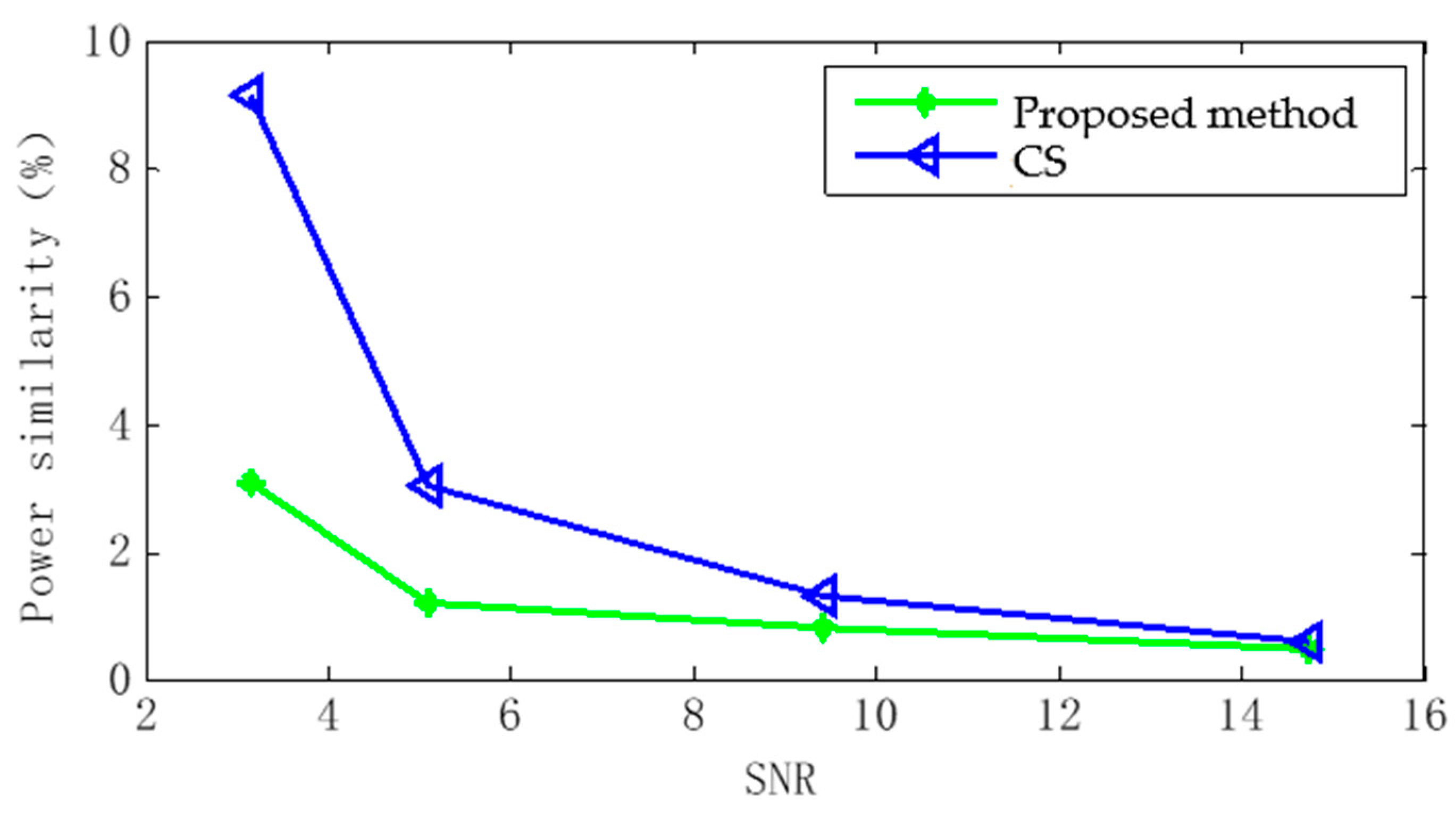
To further illustrate the effectiveness of the proposed approach, the Power Similarity method is calculated to prove the superiority of the proposed method. The Power Similarity is described as follows:
Q = ( P n P c ) P c
where Pc is the extended spectrum of the seismic data without noise, Pn is the extended spectrum of the seismic data with noise, generally, Pc, Pn ∈ [0 10 Hz]. The smaller Q is, the greater the similarity is. Figure 10 quantitatively compares the Power Similarity of the two methods under different SNR. It can be seen that the similarity of low-frequency spectrum energy extended by the two methods are gradually decreases with the decrease of SNR. The similarity decline speed of the proposed method is slower, which indicates that the effect of low-frequency expansion is better.
In summary, when the SNR of seismic data is high, both methods can accurately estimate the reflection coefficient and effectively extend the low-frequency information. With the decrease in the SNR, the accuracy of the reflection coefficient obtained by the inversion method based on CS gradually reduced. However, accuracy of the reflection coefficient obtained by the proposed method is less affected and can estimate the reflection coefficient more accurately. The expansion effect of low-frequency information is better; that is, its anti-interference ability is stronger.

4.2. Field Data Example

The field data consists of 100 traces, and the sampling interval is 2 ms. The low frequency expansion method based on CS and the proposed method are used to extend the low-frequency.
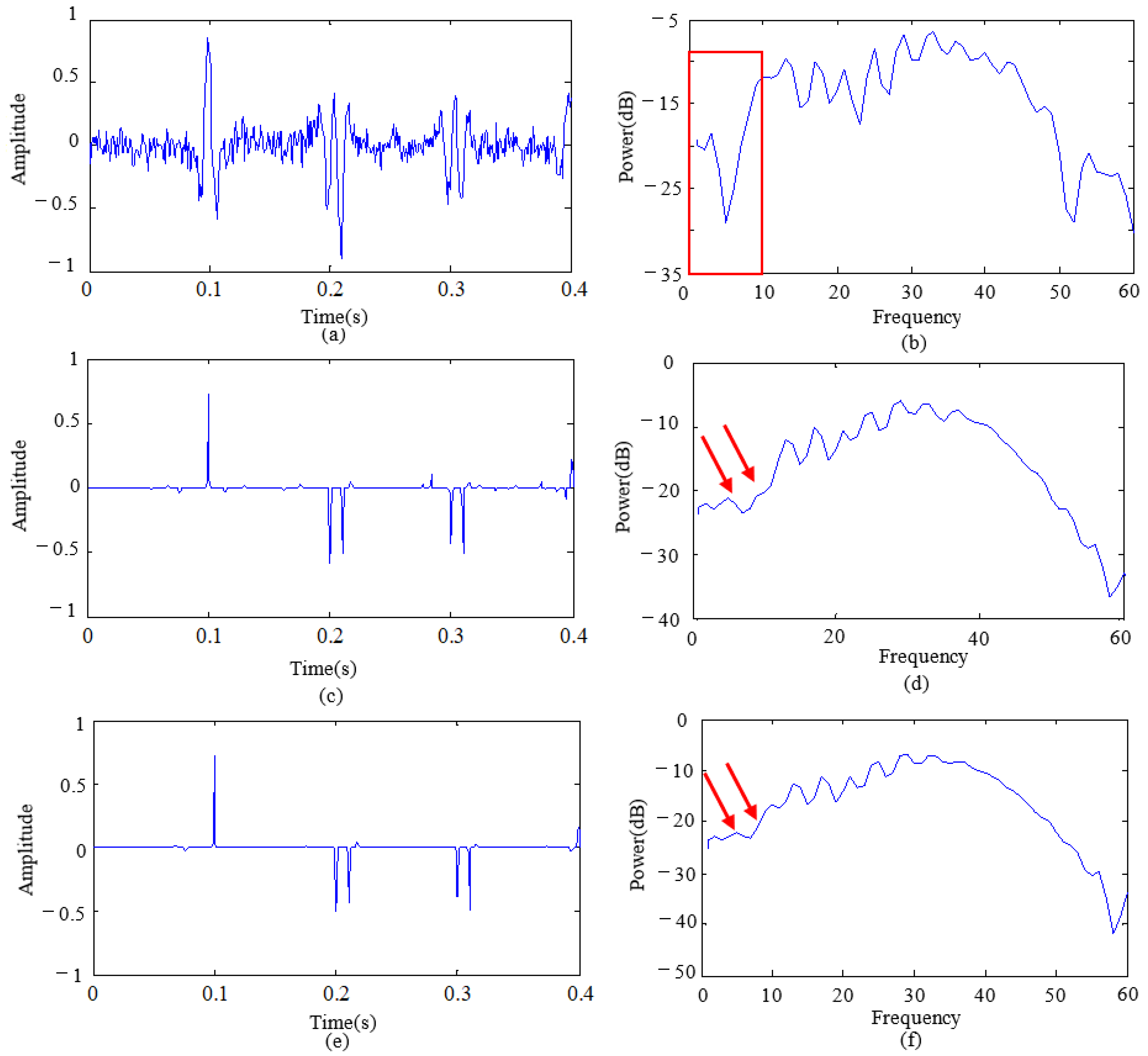
Figure 11a,b shows the actual single piece of trace data and its spectrum. It can be seen that the energy of the seismic record is relatively weak at about 5 Hz. The low-frequency expansion method based on CS can effectively extend the low-frequency information, and the energy of the signal about 5 Hz is improved to a certain extent. The proposed method can effectively extend the low-frequency information of 0–10 Hz as a whole.
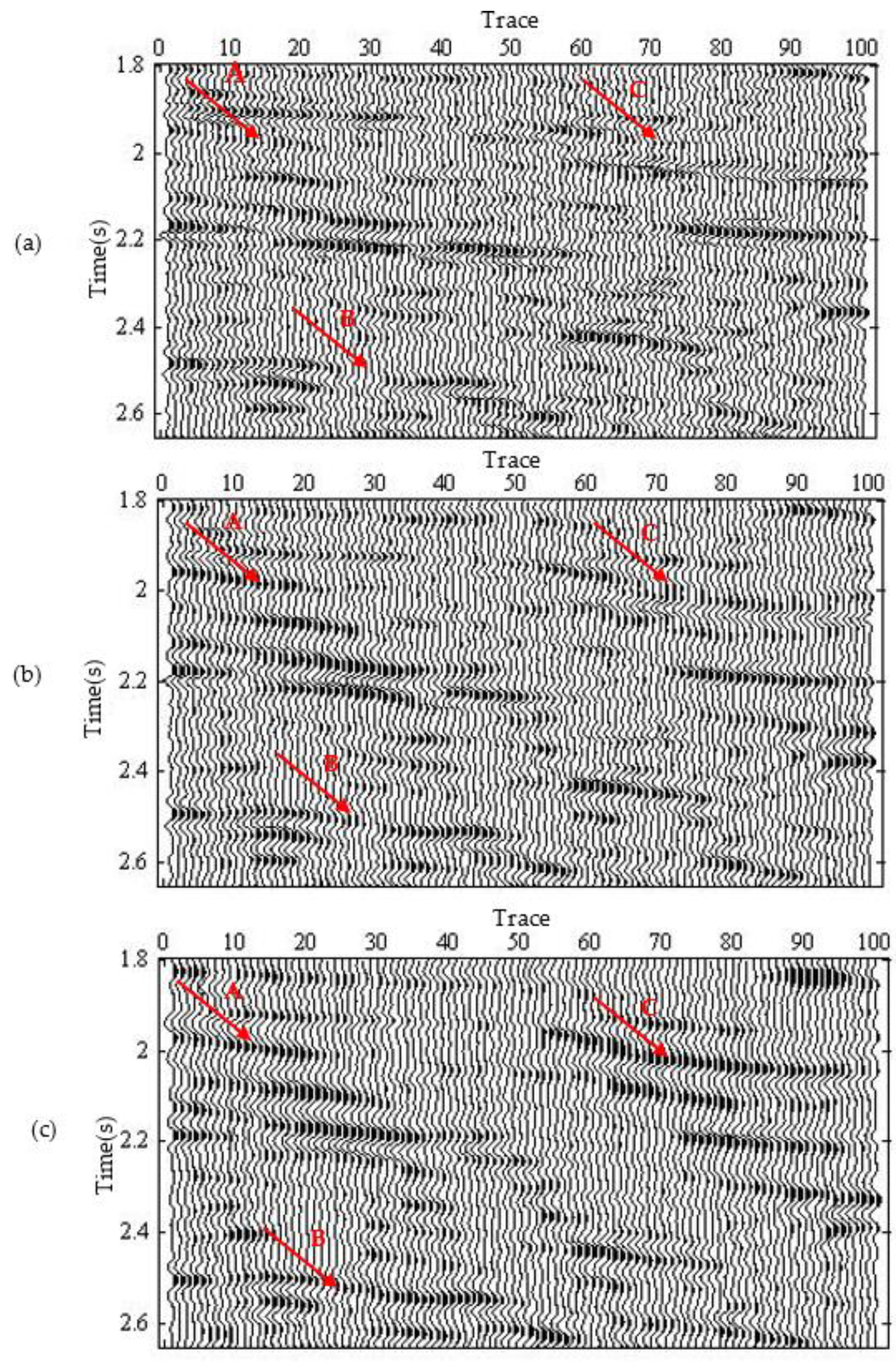
Due to the limited energy of the extended low-frequency information, it is not easy to show in the full frequency section, so the seismic records are displayed by low frequency filtering. Figure 12a shows the filtering results of the original seismic profile at 2–10 Hz. Figure 12b,c shows the low-frequency expansion results processed by the method based on CS and the proposed method. Through comparative analysis, the following points can be seen:
(1)
The seismic event at position A in the original section is discontinuous, so it is difficult to judge the basic trend of the formation. After the expansion of the two methods, energy of the seismic event at this position is significantly enhanced, and the basic trend of the formation is clear.
(2)
The seismic event at B in the original section are also discontinuous, and the continuity has been improved to a certain extend after CS low-frequency expansion. In the proposed method, the inversion process of the reflection coefficient is constrained by the well data, and the continuity of the seismic event after expansion is substantially improved.
(3)
The seismic event at the position C is not obvious. After expansion processing of CS method, the low-frequency energy is improved, but the continuity is still poor. After the expansion processing of the proposed method, the continuity of the event is significantly improved, and the effect of the low-frequency expansion is the best.
To highlight the effectiveness of the proposed approach, the segment B is taken out and shown in Figure 13. As shown in Figure 13a, the continuity of the seismic event between traces 25 and 34 in the profile is poor. After expansion processing of CS method, the energy of the seismic event between trace 25 and 34 is improved, and the continuity of the seismic event is enhanced. The proposed method can further improve the energy of the seismic event between traces 25 and 34, so as to better reflect the trend of the formation.
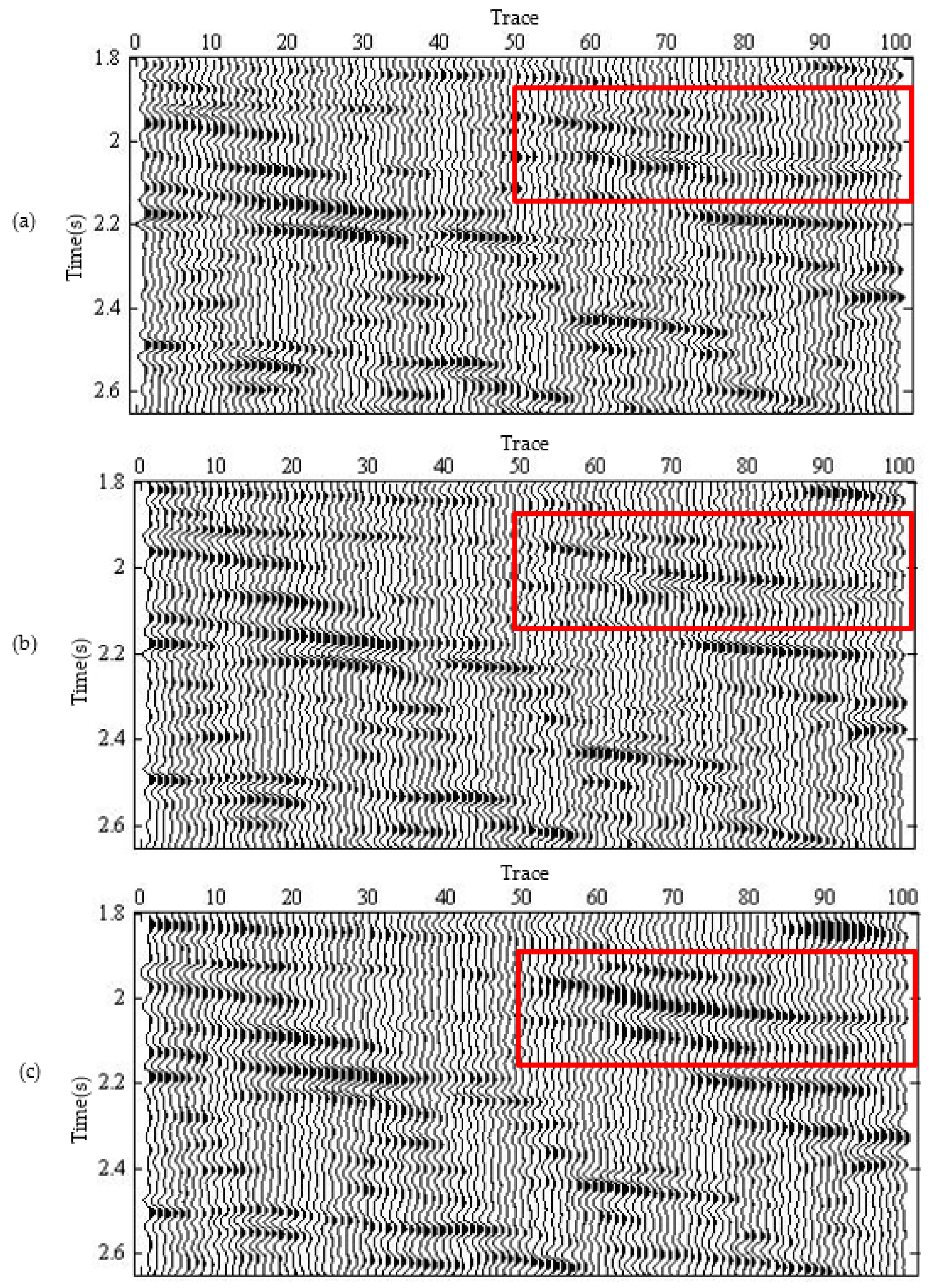
Similarly, 1–3 Hz information is taken from the original section (as shown in Figure 14), where a, b and c are the 1–3 Hz information in the original seismic section of the work area, the low-frequency expansion result based on CS and the low-frequency expansion result of the proposed method. The three seismic events framed in the figure have poor continuity. After using the CS method, the energy of low-frequency information is enhanced, and the continuity of the event is improved. After using the proposed method, the energy of low-frequency information is further enhanced, and the resolution has better promotion.

5. Conclusions

Low-frequency information can reflect the basic trend of the formation and improve the accuracy of velocity analysis and deep imaging. Conventional acquisition technology shows that low-frequency information below 10 Hz in the data is seriously polluted by noise, and some low-frequency information will be lost during processing. The low-frequency expansion method based on CS can reasonably compensate the low-frequency components to improve the quality of the data. However, this method is greatly affected by noise, and can effectively extend the low-frequency information only when the SNR is high. In order to improve the anti-interference ability of the method, well information is introduced in the construction of the objective function to constrain the inversion process of estimating the reflection coefficient. Low-frequency information of the original data is extended by extracting the low-frequency information from the reflection coefficient. Model and actual data processing results show that the proposed method, restricting the reflection coefficients inversion process by the logging data, can obtain the accurate reflection coefficients, improve the anti-noise interference ability of the inversion process, and improve the extension effect of the low-frequency information even if the noise energy is large. In this paper, it is ideal to select the point where R ˜ and G are equal. In fact, the slope of the equal point needs to be considered, which is also the problem to be solved in the further.

Author Contributions

Conceptualization, M.S. and Z.L.; methodology, M.S.; validation, J.W. and Y.S.; writing, review and editing, M.S. and Y.L.; funding acquisition, Z.L.; supervision, M.S. All authors have read and agreed to the published version of the manuscript.

Funding

This work was supported by National Natural Science Funding (NSF) under grant 41974145 and the Major Scientific and Technological Projects of CNPC (ZD2019-183-003).

Data Availability Statement

Not applicable.

Conflicts of Interest

The authors declare no conflict of interest.

References

  1. Ziolkowki, A.; Hanssen, P.; Gatliff, R.; Jakubowicz, H.; Dobson, A.; Hampson, G.; Li, X.Y.; Liu, E.R. Use of low frequencies for sub-basalt imaging. Geophys. Prospect. 2003, 51, 169–182. [Google Scholar] [CrossRef]
  2. Woodburn, N.; Hardwick, A.; Travis, T. Enhanced low frequency signal processing for sub-basalt imaging. In Proceedings of the 81th SEG Annual Meeting, San Antonio, TX, USA, 18–23 September 2011; pp. 3673–3677. [Google Scholar]
  3. Liu, H.; Liu, X. Depth-Extrapolation-Based True-Amplitude Full-Wave-Equation Migration from Topography. Appl. Sci. 2021, 11, 3010. [Google Scholar] [CrossRef]
  4. Huang, J.; Cui, C.; Liu, M. A hybrid multi-scale full waveform inversion method based on frequency-wavenumber filter and its implementation strategies. J. China Univ. Pet. 2018, 42, 50–59. [Google Scholar]
  5. Zhang, J.; Zhang, B.; Zhang, Z.; Liang, H.; Ge, D. Low-frequency data analysis and expansion. Appl. Geophys. 2015, 12, 212–220. [Google Scholar] [CrossRef]
  6. Liu, C.; Zhou, W.; Niu, C.; Long, D.; Wu, N. Cepstral time-frequency domain deconvolution based on improved generalized S-transform. J. China Univ. Pet. 2018, 42, 57–64. [Google Scholar]
  7. Wang, D.; Kong, X.; Dong, L.; Chen, L.; Wang, Y.; Wang, X. A predictive deconvolution method for non-white-noise reflectivity. Appl. Geophys. 2019, 16, 115. [Google Scholar] [CrossRef]
  8. Silvia, M.T.; Robinson, E.A. Deconvolution of geophysical time series in the exploration for oil and natural gas. Geo-Exploration 1980, 18, 77–78. [Google Scholar]
  9. Wiggins, R.A. Minimum entropy deconvolution. Geo-Exploration 1978, 16, 21–35. [Google Scholar] [CrossRef]
  10. Claerbourt, J.F. Parsimonious deconvolution. Stanf. Explor. Proj. 1977, 13, 1–9. [Google Scholar]
  11. Gray, W. Variable Norm Deconvolution. Ph.D. Thesis, Stanford University, Stanford, CA, USA, 1979. [Google Scholar]
  12. Ooe, M.; Ulrych, T.J. Minimum entropy deconvolution with an exponential transfrom. Geophys. Prospect. 2010, 27, 458–473. [Google Scholar] [CrossRef]
  13. Godfrey, R. An information theory approach to deconvotion. Stanf. Explor. Proj. 1978, 15, 157–182. [Google Scholar]
  14. Walden, A.T. Non-Gaussian reflecticity, entrory, and deconvolution. Geophysics 1985, 50, 2862–2888. [Google Scholar] [CrossRef]
  15. Larue, A.; Mars, J.I.; Jutten, C. Frequency-domain blind deconvolution based on mutual information rate. IEEE Trans. Signal Process. 2006, 54, 1771–1781. [Google Scholar] [CrossRef]
  16. Mirko, V.; Pham, D.T. Robust wavelet estimation and blind deconvolution of noisy surface seismic. Geophysics 2008, 73, V37–V46. [Google Scholar]
  17. Rosa, A.; Ulrych, T.J. Processing via spectral modeling. Geophysics 1991, 56, 1244–1251. [Google Scholar] [CrossRef]
  18. Guan, L.; Tang, Q. High/Low frequency compensation of seismic signal. Geophys. Prospect. Pet. 1990, 29, 35–45. [Google Scholar]
  19. Masoomzadeh, H.; Barton, P.; Singh, S. Preservation of low frequencies in wide-angle data processing for sub-basalt imaging. In Proceedings of the 76th SEG Annual Meeting, New Orleans, LA, USA, 1–6 October 2011; pp. 2832–2836. [Google Scholar]
  20. Guo, S.; Wang, L.; Han, W. Analysis on optimization processing method of prestack data. Geophys. Prospect. Pet. 2006, 45, 497–502. [Google Scholar]
  21. Han, L.; Zhang, Y.; Han, L.; Yu, Q. Compressed sensing and sparse inversion based low-frequency information compensation of seismic data. J. Jilin Univ. 2012, 42, 259–264. [Google Scholar]
  22. Ahmad, N.; Khan, S.; Al-Shuhail, A. Seismic Data Interpretation and Petrophysical Analysis of Kabirwala Area Tola (01) Well, Central Indus Basin, Pakistan. Appl. Sci. 2021, 11, 2911. [Google Scholar] [CrossRef]
  23. Zhang, Y.; Luo, Y.; Ling, F. Seismic trace multi-scale inversion using logging data and seismic data. Earth Sci. 2001, 26, 533–537. [Google Scholar]
  24. Pedersen-Tatalovic, R.; Uldall, A.; Jacobsen, N.L.; Hansen, T.M.; Mosegaard, K. Event based low frequency impedance modeling using well logs and seismic attributes. Lead. Edge 2008, 27, 592–603. [Google Scholar] [CrossRef] [Green Version]
  25. Donoho, D.L. Compressed sensing. IEEE Trans. Inf. Theory 2006, 52, 1289–1306. [Google Scholar] [CrossRef]
  26. Candès, E.; Romberg, J.; Tao, T. Stable signal recovery from incomplete and inaccurate measurements. Commun. Pure Appl. Math 2005, 99, 1207–1223. [Google Scholar] [CrossRef] [Green Version]
  27. Candès, E.J.; Romberg, J. Practical Signal Recovery from Random projections. Proc. SPIE Int. Soc. Opt. Eng. 2004, 5674, 76–86. [Google Scholar]
  28. Donoho, D.L.; Huo, X. Uncertainty principles and ideal atomic decomposition. IEEE Trans. Inf. Theory 2001, 47, 2845–2862. [Google Scholar] [CrossRef] [Green Version]
  29. Bi, X.; Leng, L.; Kim, C.; Liu, X.; Du, Y.; Liu, F. Constrained backtracking matching pursuit algorithm for image reconstruction in compressed sensing. Appl. Sci. 2021, 11, 1435. [Google Scholar] [CrossRef]
  30. Candès, E.J. The restricted isometry property and its implications for compressed sensing. Comptes Rendus Math. 2008, 346, 589–592. [Google Scholar] [CrossRef]
  31. Baraniuk, R.; Davenport, M.; Devore, R.; Wakin, M. A simple proof of the restricted isometry property for random matrices. Constr. Approx. 2007, 23, 91–925. [Google Scholar] [CrossRef] [Green Version]
  32. Kirachaiwanich, D.; Liang, Q. Compressive sensing: To compress or not to compress. In Proceedings of the Forty-Fifth Asilomar Conference on Signals, Systems and Computers (ASILOMAR), Pacific Grove, CA, USA, 6–9 November 2011; pp. 809–813. [Google Scholar]
  33. Herrmann, F.J.; Hennenfent, G. Non-parametric seismic data recovery with curvelet-frames. Geophys. J. Int. 2008, 173, 233–248. [Google Scholar] [CrossRef] [Green Version]
  34. Tropp, J.; Gilbert, A. Signal Recovery from Partial Information via Orthogonal Matching Pursuit. IEEE Trans. Inf. Theory 2007, 53, 4655–4666. [Google Scholar] [CrossRef] [Green Version]
  35. Davenport, M.A.; Needell, D.; Wakin, M.B. Signal space CoSaMP for sparse recovery with redundant dictionaries. IEEE Trans. Inf. Theory 2013, 59, 6820–6829. [Google Scholar] [CrossRef] [Green Version]
  36. Li, Q.; Huang, J.; Li, Z.; Li, N. 3D multi-source least-squares reverse time migration based on L1 norm regularization. J. China Univ. Pet. 2019, 43, 52–59. [Google Scholar]
  37. Gorodnitski, I.F.; Rao, B.D. Sparse signal reconstruction from limited data using focuss: A reweighted norm minimization algorithm. IEEE Trans. Signal. Process. 1997, 45, 600–616. [Google Scholar] [CrossRef] [Green Version]
  38. Moshtaghpour, A.; Jacques, L.; Cambareri, V.; Degraux, K.; Vleeschouwer, C.D. Consistent basis pursuit for signal and matrix estimates in quantized compressed sensing. IEEE Signal. Process. Lett. 2016, 23, 25–29. [Google Scholar] [CrossRef] [Green Version]
  39. Blumensath, T.; Davies, M.E. Iterative hard thresholding for compressed sensing. Appl. Comput. Harmon. Anal. 2009, 27, 265–274. [Google Scholar] [CrossRef] [Green Version]
  40. Jiao, X.; Du, Q.; Zhao, Q. Compressed sensing seismic data reconstruction based on maximum correntropy criterion. J. China Univ. Pet. 2020, 44, 38–46. [Google Scholar]
  41. Cao, J.; Wang, S.; Li, W. Seismic reconstruction with 3D low-redundancy curvelet transform and compressed sensing theory. J. China Univ. Pet. 2017, 41, 61–68. [Google Scholar]
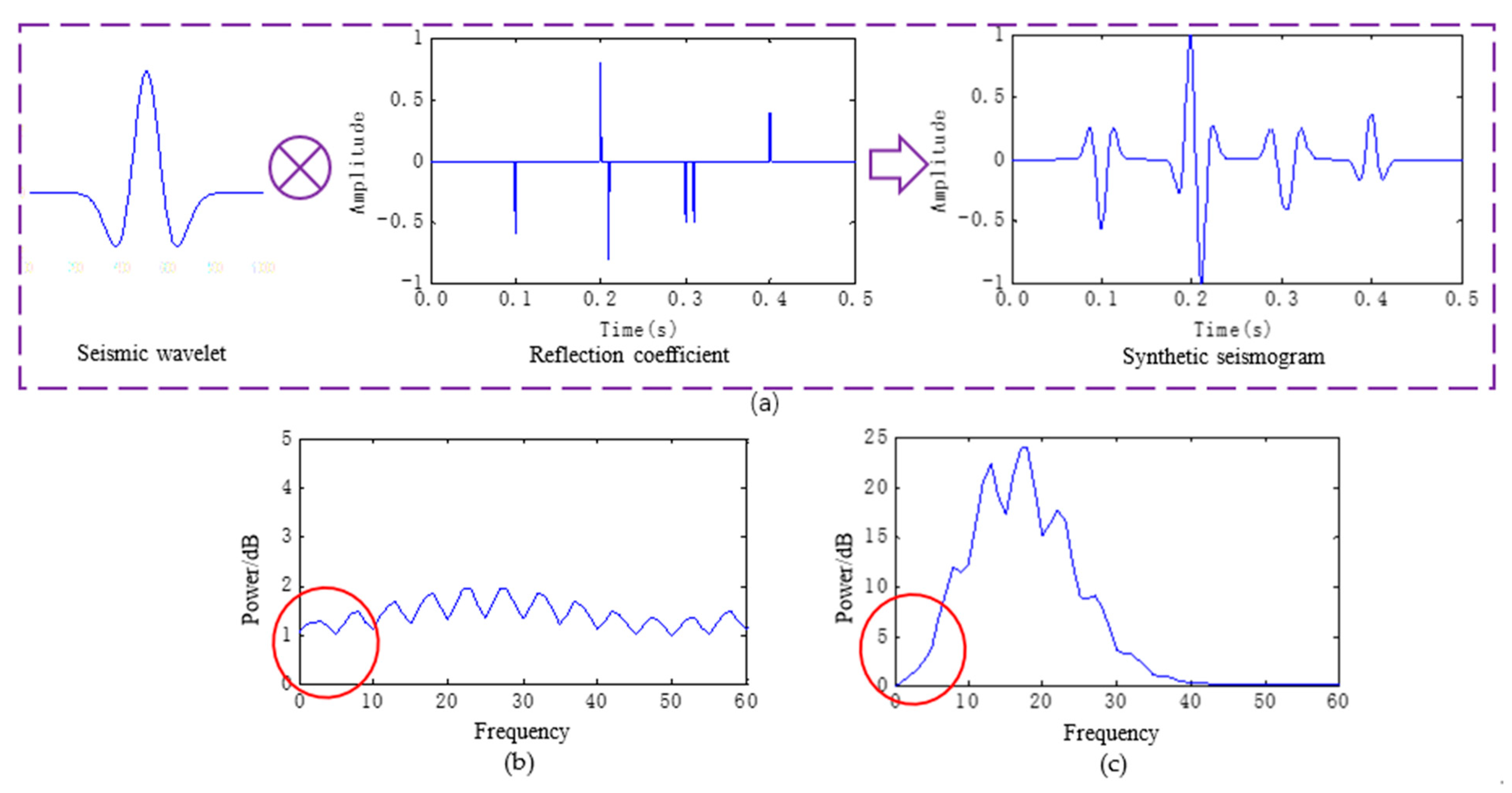
Figure 1. Schematic diagram of synthetic seismogram. (a) Convolution, (b) frequency spectrum of seismic reflection coefficient, (c) frequency spectrum of seismic wavelet.
Applsci 11 05028 g001
Figure 2. Low-frequency expansion process based on CS [21].
Applsci 11 05028 g002
Figure 3. Low-frequency expansion process with well constraint based on CS.
Applsci 11 05028 g003
Figure 4. Simulated seismic data. (a) Model data, (b) reflection coefficient model, (c) frequency spectrum of (a).
Applsci 11 05028 g004
Figure 5. Simulated seismic data after frequency-broadening processing. (a) Model data, (b) frequency spectrum of (a).
Applsci 11 05028 g005
Figure 6. Comparisons of low frequency expansion when SNR = 14.72. (a,b) Noisy data and their frequency spectrum, (c,d) reflection coefficients estimated by CS and extended spectrum, (e,f) reflection coefficients estimated by proposed method and extended spectrum.
Applsci 11 05028 g006
Figure 7. Comparisons of low-frequency expansion when SNR = 9.41. (a,b) Noisy data and their frequency spectrum, (c,d) reflection coefficients estimated by CS and extended spectrum, (e,f) reflection coefficients estimated by proposed method and extended spectrum.
Applsci 11 05028 g007
Figure 8. Comparisons of low-frequency expansion when SNR = 5.10. (a,b) Noisy data and their frequency spectrum, (c,d) reflection coefficients estimated by CS and extended spectrum, (e,f) reflection coefficients estimated by proposed method and extended spectrum.
Applsci 11 05028 g008
Figure 9. Comparisons of low frequency expansion when SNR = 3.14. (a,b) Noisy data and their frequency spectrum, (c,d) reflection coefficients estimated by CS and extended spectrum, (e,f) reflection coefficients estimated by proposed method and extended spectrum.
Applsci 11 05028 g009
Figure 10. Comparison of power spectrum similarity under different SNR.
Applsci 11 05028 g010
Figure 11. Comparisons of low-frequency expansion analysis for actual single trace record. (a) Noisy data, (b) frequency spectrum of original data, (c) data processed by CS, (d) frequency spectrum of (c), (e) data processed by the proposed method, (f) frequency spectrum of (e).
Applsci 11 05028 g011
Figure 12. Filtering profile with 2–10 Hz of actual data before and after low frequency expansion. (a) Original data, (b) processed data by CS, (c) processed data by the proposed method.
Applsci 11 05028 g012
Figure 13. Partial enlargement effect at position B in 2–10 Hz filtering profile before and after low-frequency expansion. (a) Original data, (b) processed data by CS, (c) processed data by the proposed method.
Applsci 11 05028 g013
Figure 14. Filtering profile with 1–3 Hz of actual data before and after low-frequency expansion. (a) Original data, (b) processed data by CS, (c) processed data by the proposed method.
Applsci 11 05028 g014
Publisher’s Note: MDPI stays neutral with regard to jurisdictional claims in published maps and institutional affiliations.