Article

Low-Latency Bit-Accurate Architecture for Configurable Precision Floating-Point Division

1
Shenzhen Key Laboratory of IoT Key Technology, Harbin Institute of Technology, Shenzhen 518000, China
2
School of Microelectronics, Shenzhen Institute of Information Technology, Shenzhen 518000, China
*
Authors to whom correspondence should be addressed.
Appl. Sci. 2021, 11(11), 4988; https://doi.org/10.3390/app11114988
Submission received: 21 April 2021 / Revised: 24 May 2021 / Accepted: 26 May 2021 / Published: 28 May 2021
(This article belongs to the Section Electrical, Electronics and Communications Engineering)

Abstract

:
Floating-point division is indispensable and becoming increasingly important in many modern applications. To improve speed performance of floating-point division in actual microprocessors, this paper proposes a low-latency architecture with a multi-precision architecture for floating-point division which will meet the IEEE-754 standard. There are three parts in the floating-point division design: pre-configuration, mantissa division, and quotient normalization. In the part of mantissa division, based on the fast division algorithm, a Predict–Correct algorithm is employed which brings about more partial quotient bits per cycle without consuming too much circuit area. Detailed analysis is presented to support the guaranteed accuracy per cycle with no restriction to specific parameters. In the synthesis using TSMC, 90 nm standard cell library, the results show that the proposed architecture has ≈63.6% latency, ≈30.23% total time (latency × period), ≈31.8% total energy (power × latency × period), and ≈44.6% efficient average energy (power × latency × period/efficient length) overhead over the latest floating-point division structure. In terms of latency, the proposed division architecture is much faster than several classic processors.

1. Introduction

Modern applications comprise several floating-point (FP) operations including FP addition, multiplication, and division. In recent FP units, emphasis has been placed on designing ever-faster adders and multipliers, with division receiving less attention. Typically, the range for FP addition latency is two to four cycles, and the range for FP multiplication is two to eight cycles [1]. In contrast, the latency for double precision division in modern floating point units ranges from less than eight cycles to over 60 cycles [2].
Literature exists describing division algorithms, of which digit recurrence, functional iteration, variable latency, very high radix, and look-up table are five typical division implementations [3].
Digit-recurrence algorithm is based on iterative subtraction, including restoring [4], non-restoring [5], and Sweeney-Robertson-Tocher (radix-n SRT) algorithm (SRT is in fact one of non-restoring algorithms) [6]. It works digit by-digit with an iterative-type subtraction and produces a quotient in sequence [7]. According to [8], digit-recurrence algorithm of low radix is likely to cause long latency when encountering high-precision calculation due to its linear convergence speed. In contrast, high-radix digit-recurrence algorithm can reduce latency at the expense of multifold area consumption.
Functional iteration algorithm is mainly comprised of Newton–Raphson [9,10], Goldschmidt [11,12], Series expansion [13], and Taylor series algorithm [14,15]. A functional iteration divider computes the quotient of division by prediction; thus, based on multiplication instead of subtraction, it can give more than one digit of the quotient in one iteration, which ultimately reduces the iterations greatly [8,9,12]. According to [8], since they have square convergence, the faster convergence speed brings low delay. However, higher hardware requirements are put forwards at the same time.
The Digital Equipment Corporation (DEC) Alpha 21164 [16] is one of the best examples of variable latency class algorithm implementation. It is found in [17] that the average number of quotient bits retired in one iteration varies from 2 to 3 depending on the stream of bits in the partial remainder. There are certain ways in [17] to provide a variable conversion time in variable latency algorithm: self-timing, result cache, and speculation of quotient digit.
Generally, a divider retiring more than 10 quotient digits in one iteration qualifies as a very high-radix algorithm [2,18,19]. As with low-radix SRT algorithm, a very high-radix algorithm also uses a look-up table. In [20], the main difference between SRT and very high-radix algorithm is that it has a more complex divisor multiple processing and quotient-digit selection hardware, which increases the cycle time and area.
A look-up table algorithm [21,22,23,24,25] can be used along with digit recurrence, functional iterative, and very high-radix algorithms. Take SRT radix-n division algorithm, the approximation can be achieved by a look-up table that can provide a faster option at the expense of an increased area [26,27]. Additionally, the look-up table area also increases as the number of bits increases.
Our research focuses on the architecture design of configurable precision FP arithmetic units. Several papers have proposed FP architectures on the idea of multi-precision FP arithmetic processing. Most prior works are focused on the adder architectures [28,29,30,31,32] and multiplier architectures [33,34,35,36].
This paper focuses on the design of configurable multi-precision FP divider. The proposed architecture is based on very high-radix algorithm [18], which can work out much more than 10-bit quotient in one clock cycle. The proposed architecture is designed for normal as well as subnormal computational support, which also includes the exceptional case handling and processing. The major building blocks (like PRECONFIG, MANTISSA_DIVIDE, and NORMALIZE) are designed and optimized for the low-latency and bit-accurate purpose. Some techniques are applied in the hardware architecture design:
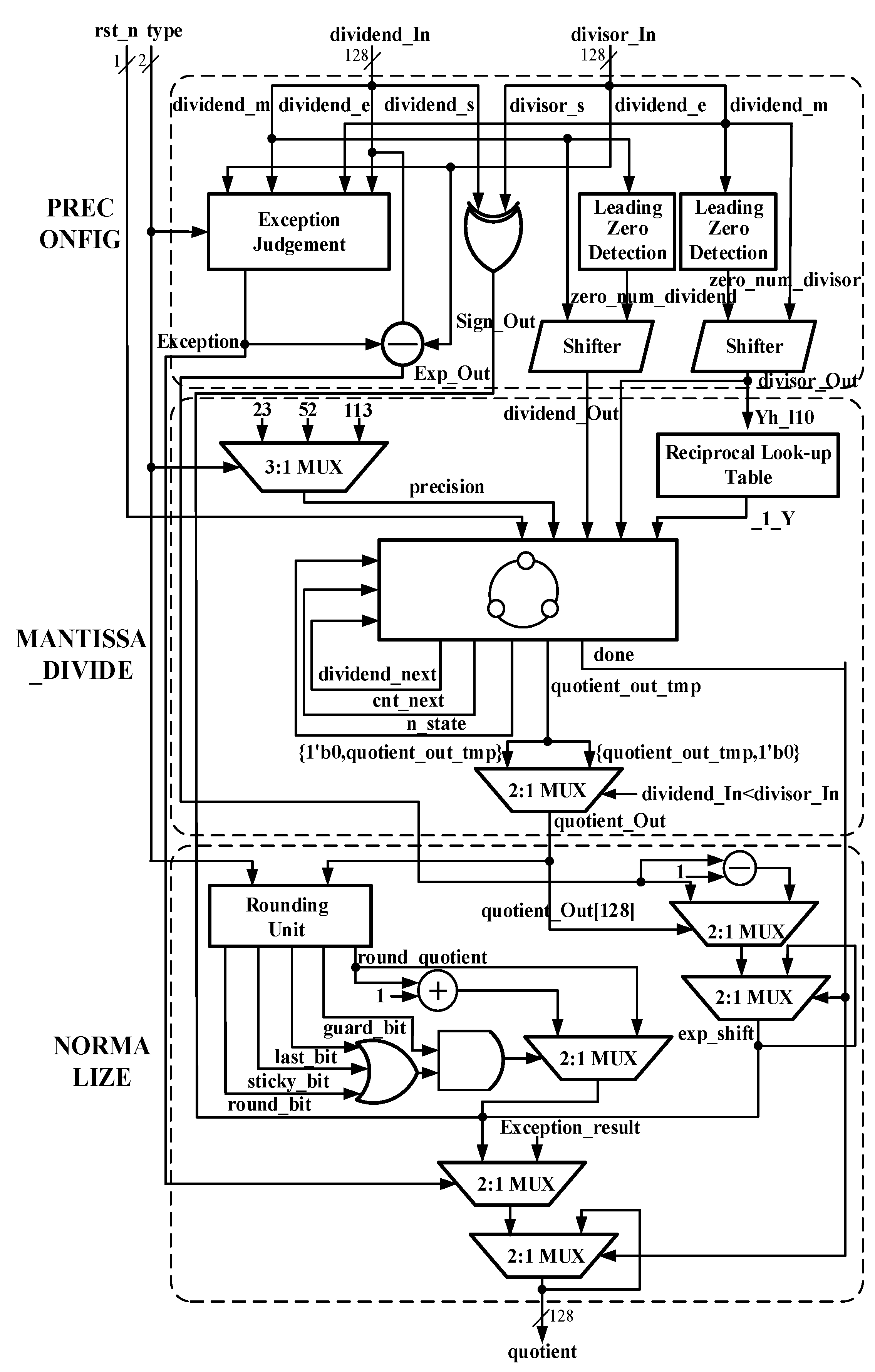
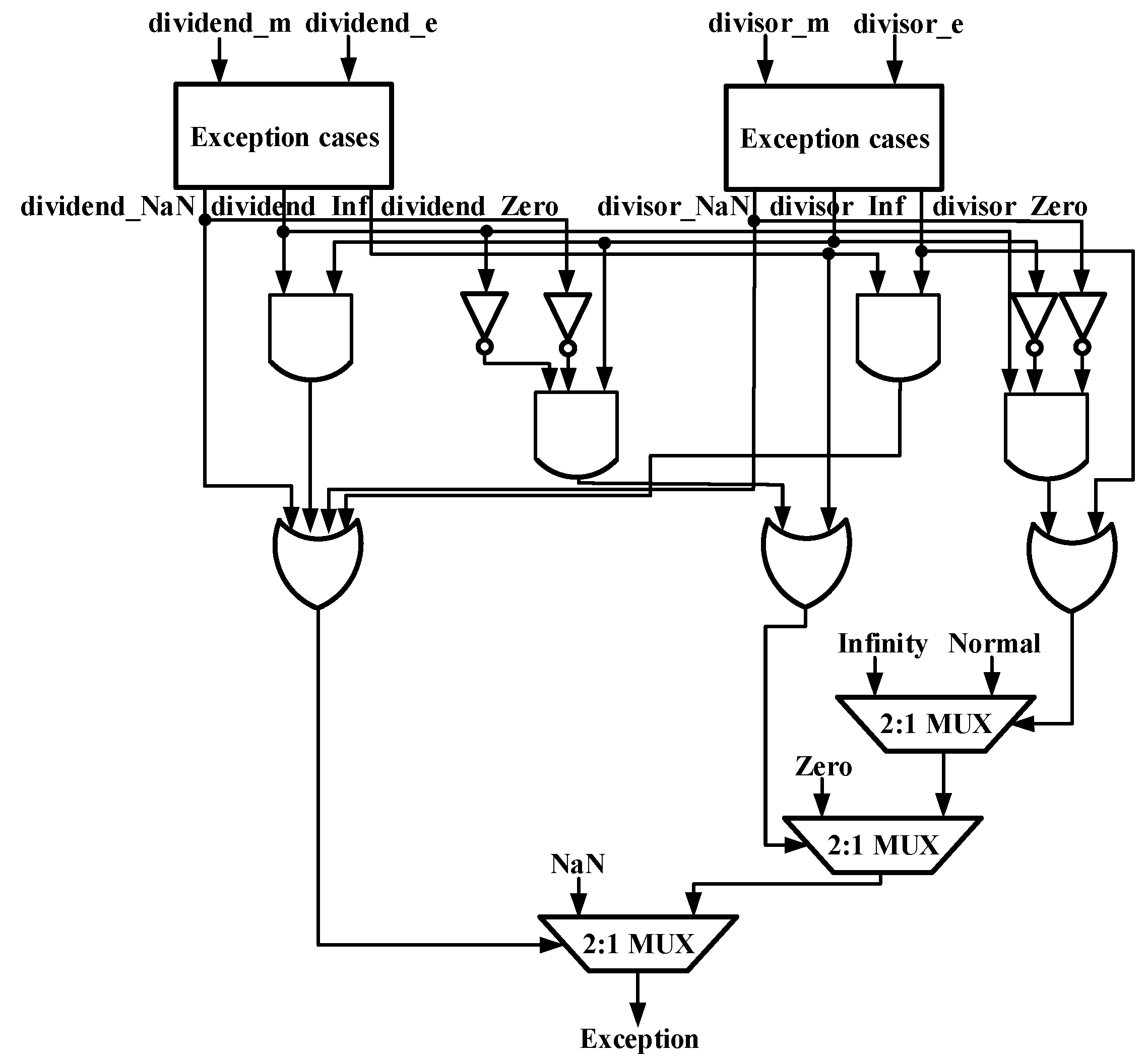
  • Leading Zero Detection module to transfer subnormal inputs; Exception Judgement module to check exception conditions;
  • Finite State Machine module to reduce the number of multipliers and to perform basic fast division steps;
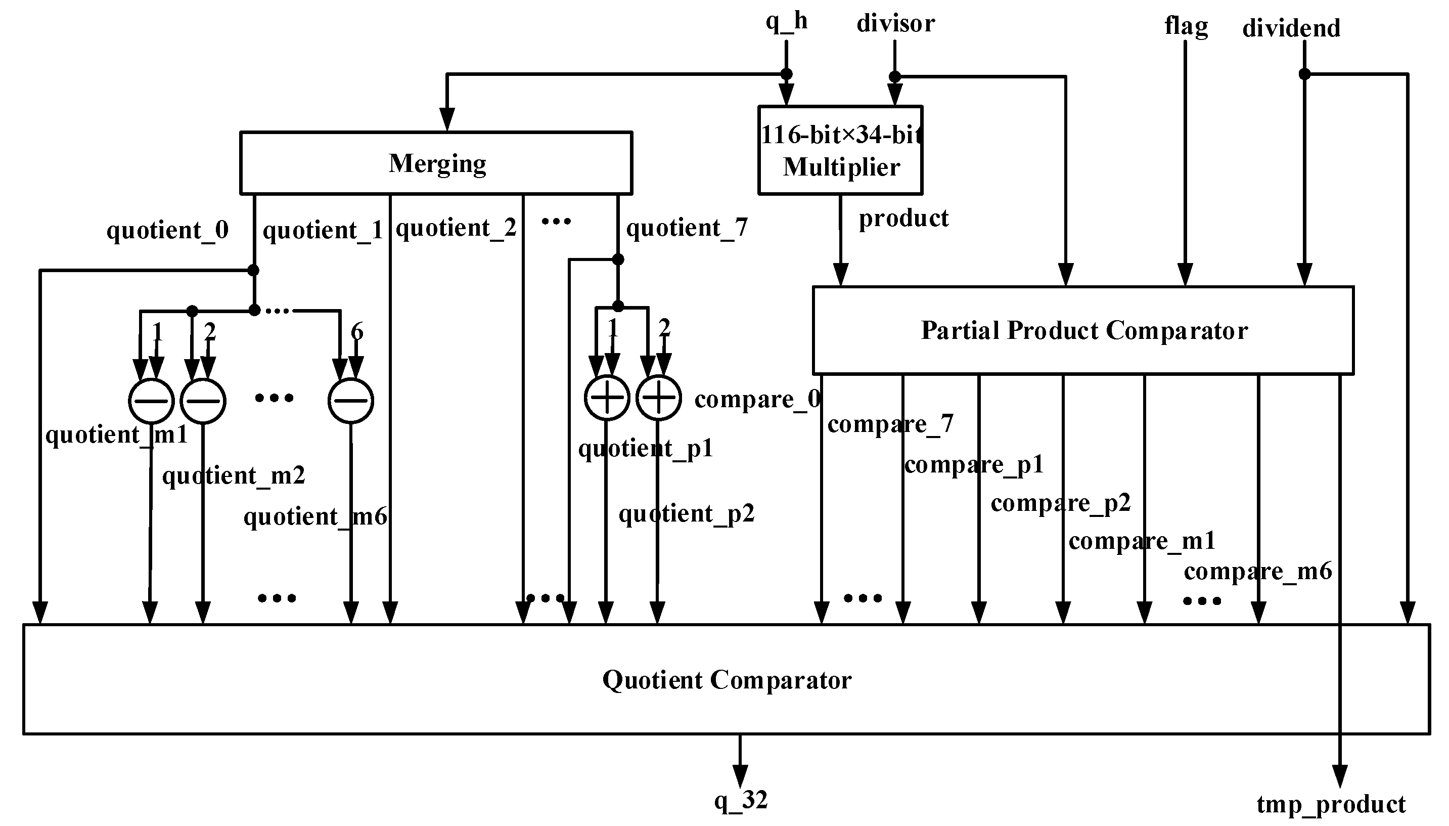
  • Quotient Selection Unit module to finish the critical part of our proposed Predict–Correct algorithm and to gain the most approximative 32-bit quotient per cycle;
  • Rounding Unit module to ensure the accuracy of unit at last place of quotient.
The remaining paper is structured as follows. In Section 2, two classical division implementations employing very high-radix algorithm are reviewed and higher radix division implementation is discussed. In Section 3, a novel Predict–Correct algorithm based on fast division and its mathematical arguments are presented. In Section 4, general architecture of the proposed multi-precision FP division and its main techniques are detailed. In Section 5, the results of our hardware implementation are reported and compared with prior works. Finally, in Section 6, conclusion is drawn.

2. Background

Very high-radix class algorithm is similar to non-restoring digit-recurrence algorithm. Their differences lie in hardware and logic arrangements for quotient selection and partial remainder generation. A simple basic schematic of very high-radix class algorithm is presented in Figure 1.
Proposed by Wong and Flynn, fast division [18] is the earliest high-radix algorithm. Fast division requires hardware with at least one look-up table of size 2m−1 × m bits and three multipliers, a carrying assimilation multiplier of size (m + 1) × n for the divisor’s initial multiplications and a carry-save multiplier of size (m + 1) × m for the quotient segments computation. As for the basic version of fast division, the look-up table has m = 11, i.e., 2(11−1) = 1024 entries, each 11 bits wide, so in total, 11 K bits are required in the look-up table. As for the advanced version, 736 K bits are required in the look-up table when m = 16.
The high-radix algorithm proposed by Lang and Nannarelli [19] shows the construction of a radix-2K divider for implementing a radix-10 divider whose quotient digit is decomposed into two parts, one in radix-5 and the other in radix-2. In radix-5, the quotient digit is represented as values {−2, −1, 0, 1, 2}, requiring three multipliers. Radix-2 is used to perform division on the most significant slice. It uses an estimation technique in the quotient selection component, which requires the use of a redundant digit format.
In brief, high-radix division algorithm works with a scaling dividend and divisor by correct initial approximation of the reciprocal, followed by quotient selection logic with a multiplier and subtraction. Beyond this, high-radix dividers are almost the same as SRT-based radix dividers.
When it comes to ways to implement higher radix dividers, prior works focus on enhancing the complexity and criticality of SRT-based radix dividers [37,38]. Moreover, a combination of two or more alternatives together could be another way. Many works are going on to provide different standpoints for high-radix dividers. Use of different look-up tables along with quotient-digit selection logic look-up table [39,40,41], speculating quotient digit and using arithmetic functions to multiplicative iterations rather than subtractive iterations [42], pre-scaling operands [43,44,45], using Fourier division [46,47], using alternative digit codes such as binary-coded decimal (BCD) digits instead of decimal and basic binary digits [48], cascading multiple stages of lower radix dividers [49], overlapping two or more stages of low radix [50,51], a truncated schema of exact cell binary shifted adder array [52,53,54], on-line serial and pipelined operand division [55], parallel implementation of the low-radix dividers [8], array implementation [56], these are some of the possible ways applicable for high-radix dividers.

3. Predict–Correct Algorithm for Division

Inspired by fast division method [18], this paper proposes a Predict–Correct algorithm which will increase iteration speed by bringing about n more quotient bits than fast division without consuming many areas.
Our proposed division is similar to fast division in that both use multiplication for divisor multiple formation and look-up tables to obtain an initial approximation to the reciprocal of divisor. Their differences lie in the number and type of subsequent operations used in each cycle and the technique used for quotient-digit selection.

3.1. Predict–Correct Algorithm with Accurate Quotient Approximation

In the Predict–Correct algorithm, truncated versions of the integer dividend X and divisor Y are used, denoted Xh and Yh. Xh is defined as the high-order p bits of X extended with 0s to obtain a q-bit number, i.e., Xh = X(q−1)X(qp)00…00 where the number of 0 in Xh is qp. Similarly, Yh is defined as the high-order m bits of Y extended with 1s to obtain a q-bit number, i.e., Yh = Y(q−1)Y(qm)11…11 where the number of 1 in Yh is qm.
Due to the definitions, Xh is always less than or equal to X, and Yh is always greater than or equal to Y. Let ∆X = XXh and ∆Y = YYh. The deltas ∆X and ∆Y are the adjustments needed to obtain the true X and Y from Xh and Yh. This implies that ∆X is always nonnegative and ∆Y nonpositive. The fraction 1/Yh is always less than or equal to 1/Y, and, therefore, Xh/Yh is always less than or equal to X/Y.
The Taylor series approximation equation for 1/Y about Y = Yh is:
B = 1/Yh − ∆Y/Yh2 + (∆Y)2/Yh3 − (∆Y)3/Yh4 + (∆Y)4/Yh5 + ⋯ + (−1)t−1 (∆Y)t−1/Yht + ⋯.
The Predict–Correct algorithm (Algorithm 1) is conceptually summarized as follows.
Algorithm 1 Predict–Correct Algorithm.
1: Set Q and j to 0 initially.
2: With index of the leading m bits of Y, look b1 bits wide approximation of 1/Yh up in the table G1.
Similarly, look b2 bits wide approximation of 1/Yh2 up in the table G2, …, look bt bits wide approximation of 1/Yht up in the table Gt.
Table sizes are bi = (m × tt) + ⌈log2t⌉ − (m × Imi), i = 1, 2, …, t, where t is the number of the used leading terms of (1). The relationship of parameter p and m is p = m × tt + 2.
3: Compute an approximation B to 1/Y using the leading t terms of (1):
B = 1/Yh − ∆Y/Yh2 + (∆Y)2/Yh3 − … + (−1)t−1 (∆Y)t−1/Yht. Truncate B to the most significant m × tt + 4 bits, which reduces the sizing of multipliers.
4: Compute intermediate value P = Xh × B and round P to m × tt − 1 bits to obtain P′.
5: List 2n kinds of (m × tt + n − 1)-bit quotients that combinate the (m × tt − 1)-bit intermediate value P′ with subsequent 2n kinds of n-bit predictive values ranging from 00…0 to 11…1.
6: Pick up the most approximative (m × tt + n − 1)-bit quotient Qa from the 2n kinds of (m × tt + n − 1)-bit quotients by multiplication and comparison.
7: Calculate j= j + m × tt + n − 1.
Update j with j′.
8: New dividend is X′ = XQa × Y.
New quotient is Q′ = Q + Qa × 1/2(qj).
9: Left-shift X′ by m × tt + n − 1 bits.
10: Update Q with Q′.
Update X with X′.
11: Repeat Step 4 through 10 until jq.
12: Final quotient is Q = Q(q−1)Q0Q−1Q−e = Qh + Ql where Qh = Q(q−1)Q0, Ql = Q−1Q−e and e is the number of redundant bits of the last cycle in Step 11.
In the Predict–Correct algorithm, Parameter t represents the number of the used leading terms of (1). For instance, if t = 2, the approximation to 1/Y is B = 1/Yh − ∆Y/Yh2; if t = 3, the approximation to 1/Y is B = 1/Yh − ∆Y/Yh2 + (∆Y)2/Yh3. Parameter m represents the digits number of the index of look-up table G1, G2, …, Gt. m plays a crucial role in the sizes of look-up table G1, G2, …, Gt. Moreover, the data width of entries in look-up table Gi is bi = (m × tt) + ⌈log2t⌉ − (m × imi), i = 1, 2, …, t. Parameter n represents the number of additional digits of quotient owing to Step 5 and 6 per iteration. For instance, if n = 2, subsequent 2n kinds of (m × tt + n − 1)-bit possible quotients are P′-00, P′-01, P′-10 and P′-11, where the most approximative quotient Qa is picked up from these possible quotients via quotient selection in Step 6.
To help to understand the abovementioned algorithm, an example of fixed-point division using the proposed Predict–Correct algorithm (Algorithm 2) is demonstrated as follows.
Algorithm 2 Example of Fixed-point division using Predict–Correct Algorithm.
X = (1 0010 0011 1110 0110 1100 0111 0101 1011)2,
Y = (1 1101 0101 1011 0010 1101 1110 0101 0010)2.
Set q = 33, p = 20, m = 7, t = 3, n = 3.
Then b1 = 21, b2 = 15, b3 = 9.
  Xh = (1 0010 0011 1110 0110 1100 0000 0000 0000)2,
  Yh = (1 1101 0111 1111 1111 1111 1111 1111 1111)2,
  ∆Y = (−0 0000 0010 0100 1101 0010 0001 1010 1101)2.
  B = 1/Yh − ∆Y/Yh2 + (∆Y)2/Yh3 and B is to be truncated to 22 bits.
1: Q = 0, j = 0.
2: 1/Yh = (0 1000 1011 1000 0011 0011)2, 1/Yh2 = (0 0100 1100 0000 100)2,
 1/Yh3 = (0 0010 1001)2.
3: B = (0 1000 1011 1000 0111 0001 1)2.
4: P = (0 1001 1111 0001 1000 0101 0100 0100 1100 1110 0010)2,
 and then P= (0 1001 1111 0001 1000)2.
5: 8 kinds of 20-bit possible quotients are:
(0 1001 1111 0001 1000 000)2
(0 1001 1111 0001 1000 001)2
(0 1001 1111 0001 1000 010)2
(0 1001 1111 0001 1000 011)2
(0 1001 1111 0001 1000 100)2
(0 1001 1111 0001 1000 101)2
(0 1001 1111 0001 1000 110)2
(0 1001 1111 0001 1000 111)2
6: Qa = (0 1001 1111 0001 1000 010)2.
7: j= 20 and Update j with j′.
8: X′ = (0000 0000 0000 0000 0000 1100 0100 0101 0010 0000 1010 1110 1110 0)2,
Q′ = (0 1001 1111 0001 1000 010)2.
9: Left-shift X′ by 20 bits.
10: Update Q and X with Q′ and X′ respectively.
11: Since j < q, repeat Step 4 through 10.
4′: P = (1101 0110 0000 0000 0011 1111 0100 1011 0110 0000)2
 and then P= (1101 0110 0000 0000 0)2.
5′: 8 kinds of 20-bit possible quotients are:
(1101 0110 0000 0000 0 000)2
(1101 0110 0000 0000 0 001)2
(1101 0110 0000 0000 0 010)2
(1101 0110 0000 0000 0 011)2
(1101 0110 0000 0000 0 100)2
(1101 0110 0000 0000 0 101)2
(1101 0110 0000 0000 0 110)2
(1101 0110 0000 0000 0 111)2
6′: Qa = (1101 0110 0000 0000 0 100)2.
7′: j= 40 and Update j with j′.
8′: X′ = (0000 0000 0000 0000 0000 0110 1010 0101 1010 1111 0001 1010 1110 0)2,
Q′ = (0 1001 1111 0001 1000 0101 1010 1100 0000 0000 100)2.
9′: Left-shift X′ by 20 bits.
10′: Update Q and X with Q′ and X′ respectively.
11′: Since j > q, stop the iteration.
13: Final quotient is Q = Qh + Ql where Qh =(0 1001 1111 0001 1000 0101 1010 1100 0000)2,
  Ql = (0000 100)2.

3.2. Guaranteed Bits per Cycle Using Predict–Correct Algorithm

There are three sources of inaccuracy affecting the approximation B ≈ 1/Y. Define the source by B = 1/YRbRcRd. Rb represents an error due to truncating the Taylor series after t terms. Since the truncated terms in the series are all nonnegative, Rb is nonnegative. Rc represents the error in using look-up table with finite width words to calculate B. As tables are rounded down, Rc is always nonnegative. Rd represents the error in truncating the arithmetic used to calculate B.
To obtain the maximal value of X, Rb, Rc, and Rd should be accurately bounded.
The (w + 1)th term of the Taylor series for B is Bw + 1 = (−∆Y)w/Yh(w + 1). The worst case occurs when −∆Y = 1/2m − 1/2q, the bound holds:
B w + 1 < 1 / 2 ( m × w ) × 1 / Y h ( w + 1 ) .
Therefore, the remainder Rb is bounded by
R b = g = t B g + 1 < g = t 1 / 2 ( m × g ) × 1 / Y h ( g + 1 ) = ( 1 / 2 ( m × t ) ) × ( 1 / Y h ) ( t + 1 ) 1 1 / ( 2 m × Y h ) .
For m >> 1,
( 1 / 2 ( m × t ) ) × ( 1 / Y h ) ( t + 1 ) 1 1 / ( 2 m × Y h )
is just greater than (1/2(m×t)) × (1/(Yh)(t+1)).
For m >> 5, a nonstringent bound can be posed on Rb:
R b < 1.1 2 ( m × t ) × Y h ( t + 1 ) .
Suppose the error in each table look-up is εi and the truncation error in computing each multiplicative term is δi. Let δ0 be an additional term that represents truncating B to a certain number of bits after the summation. A cumulative error will be
B = i = 1 t [ δ i + ( ε i + 1 / Y h i ) × ( Δ Y ) i 1 ] = i = 1 t [ ( Δ Y ) i 1 Y h i ] + i = 1 t [ ε i × ( Δ Y ) i 1 ] + i = 1 t δ i .
Then,
R c = i = 1 t ε i × ( Δ Y ) i 1 ,
and
R d = i = 1 t δ i .
Since table Gi is bi bits wide and 1/2 < Yh < 1, the maximal value of (1/Yh)i is slightly less than 2i. If words in table Gi can represent values up to but not including 2i, the unit of the most significant bit in table Gi should have value 2(i−1) while the unit of the least significant bit should have value 1/2(bi−i).
Each εi is less than the unit of the LSB: εi < 1/2(bi−i). The worst case for −∆Y occurs when −∆Y = 1/2m − 1/2q. Replace Y in (6) with 1/2m − 1/2q and yields
R c = i = 1 t   1 / 2 ( b i i ) × 1 / 2 ( m × i m ) ,
i.e.,
R c = i = 1 t   1 / 2 ( b i + m × i m i ) .
δi represents each maximal permissible truncation error and it allows the arithmetic of B to be reduced into an appropriate size to accelerate the computation of B. The allowable truncation error δi can be used both in discarding least significant partial products to prune multiplier trees and in truncating results to smaller widths.
As 1 ≤ B < 2, the most significant bit (MSB) of B has unit 1. Suppose B is truncated to bb bits. According to the definition of δ0, δ0 is less than the LSB, i.e., δ0 < 1/2(bb−1). To restrict Rd as follows: Rd < 1/2(m×tt+2), δ0 should be restricted as follows: δ0 < 1/2(m×tt+3), i.e., B can be truncated to be bb = m × t − t + 4 bits; meanwhile, the remaining δi should be restricted to:
i = 1 t δ i < 1 / 2 ( m × t t + 3 ) .
We already have
X = X Q a × Y = X ( P + S ) × Y = X P × Y S × Y ,
where S is the follow-up n-bit digits after P′ in the partial quotient Qa. Since P′ is the truncated version of P = Xh × B and X the left-shifted version of X′,
X < X P × Y = X X h × B × Y = Δ X + X h X h × ( 1 / Y R b R c R d ) × Y = Δ X + X h × ( R b + R c + R d ) × Y
Now substitute the bounds for Rb, Rc and Rd into (13) to determine the maximum value of X′. Since Xh < 1 and ∆X ≤ 1/2p − 1/2q, the worst case for X′ is:
X < Δ X + R b × Y + R c × Y + R d × Y ,
X < 1 / 2 p 1 / 2 q + 1.1 × Y 2 ( m × t ) × Y h ( t + 1 ) + Y 2 ( m × t t ) + Y 2 ( m × t t + 2 ) .
Since YhY, set Yh = Y in the worst case for X′ and yield:
X < 1 / 2 p 1 / 2 q + 1.1 2 ( m × t ) × Y t + Y 2 ( m × t t ) + Y 2 ( m × t t + 2 ) .
Take
X 2 = 1 / 2 p 1 / 2 q + 1.1 2 ( m × t ) × Y t + Y 2 ( m × t t ) + Y 2 ( m × t t + 2 ) ,
then
X < X 2 .
To determine the worst case of the value of X2 in the case of 1/2 ≤ Y < 1, all possible maxima and minima should be located through setting the partial derivative ∂X2/∂Y to zero.
It can be demonstrated that the highest possible value of X2 occurs at Y = 1/2. When p = m × tt + 2,
X < 0.25 2 ( m × t t ) 1 / 2 q + 1.725 2 ( m × t t ) ,
X < 1 / 2 ( m × t t 1 ) .
In Step 4 of every cycle, the highest-order bit of X′ that could possibly be 1 is the (m × tt)th bit, X′(qm×t+t). For any p such that pm × tt + 2, the worst case for the value of X′ is bounded by the above inequality. As a result, at least the front m × tt − 1 bits of quotient per cycle before Step 5 can be guaranteed in the proposed Predict–Correct algorithm.
According to (12) and (13),
X = X P × Y S × Y < X 2 S × Y = X 2 × S S × Y .
Since S is the follow-up n-bit digits after P′ in the partial quotient Qa, the worst case of the value of S × Y also occurs in the case of 1/2 ≤ Y < 1 after Step 5 and 6. Meanwhile, the highest possible value of X2 locates at Y = 1/2,
X 1 / 2 ( m × t t + n 1 ) 1 / 2 ( m × t t + n ) ,
X 1 / 2 ( m × t t + n ) .
Similarly, the highest-order bit of X′ that could possibly be 1 is the (m × tt + n)th bit. As for the subsequent n-bit predictive quotient values, the n-bit value is accurate within the least significant bit in Step 6. In short, at least the front m × tt + n − 1 bits of quotient per cycle after Step 6 can be guaranteed.
Fast division [18] generates new quotient by m × t – t – 1 bits per cycle. Therefore, the algorithm requires ⌈q/(m × tt − 1)⌉ cycles where q is digit amount of dividend X and divisor Y. Contrastively, the proposed Predict–Correct algorithm generates m × tt + n − 1 bits per cycle and its implementation requires ⌈q/(m × tt + n − 1)⌉ cycles theoretically.

3.3. Choice of Parameters m, t, and n in Predict–Correct Algorithm

As stated in Section 3.2, the proposed Predict–Correct algorithm generates m × tt + n − 1 bits per clock cycle. Change of Parameter m, t, or n leads to different guaranteed bits per cycle. Discussions about choice of parameters m, t, and n adopted in FP division hardware architecture are as follows.
Table 1 lists five options of Parameter n from 1 to 5. It can be seen from Table 1 that as n increases, the number of possible quotients increases exponentially. When n > 3, increase in guaranteed bits of quotient per cycle cannot make up the foreseeable extra cost of subsequent selectors accompanied with more possible quotients in Step 6. Compared with Parameter n = 2, Parameter n = 3 brings about one more guaranteed bit of quotient with only four more subsequent selectors needed. Compared with Parameter n = 3, Parameter n = 4 takes eight more subsequent selectors. One more guaranteed bit of quotient can apparently not overweigh the follow-up computational burden of eight more selectors. To sum up, Parameter n in the Predict–Correct Algorithm for FP division is chosen to be 3.
When t ≥ 5, the increase in guaranteed bits of quotient per cycle is at the cost of pre-computation of the terms in the approximation B. Pre-computation of the terms in B will definitely add more clock cycles, which is not friendly to low-precision division. When t = 1, the Predict–Correct algorithm becomes classical reciprocal method. Therefore, t = 2, 3, 4 will be discussed.
Table 2 lists different patterns of Parameter m and t when n = 3. Since this paper mainly focuses on high-precision FP division, so column clock cycles in Table 2 is analyzed based on quadruple precision FP division. When it comes to column clock cycles, the former figure represents the number of iterations in 113-bit mantissa division; the latter represents the number of cycle(s) needed in the pre-computation of the approximation B. In the case of Row 1 in Table 2, ⌈113/20⌉ = 6; t = 2 means that at least one cycle is needed to pre-compute the approximation B = 1/Yh − ∆Y/Yh2. It can be seen from Table 2 that the listed patterns of Parameter m and t have 6 or 7 clock cycles. As Parameter m increases from 10 to 11, data width of entries in look-up table (LUT) increase by 512. As Parameter m increases from 11 to 12, data width of entries in LUT increase by 1024. Apparently, the sharp increase in data width of LUT entries will bring about considerable area. Moreover, the increase in Parameter m seems to be no benefit to clock cycles. Hence, the patterns of Parameter m = 12 are not considered.
Therefore, the left four patterns are more rational: m = 10, t = 3; m = 10, t = 4; m = 11, t = 3; m = 11, t = 4. Achieved bits per cycle of patterns m = 10, t = 3 and m = 10, t = 4 are 116 and 114. Error may occur in the rounding of the iterated 116-bit or 114-bit quotient to the desired 113-bit normalized quotient. The two patterns are removed from consideration. As for patterns m = 11, t = 3 and m = 11, t = 4, the former pattern has more achieved bits per cycle than the latter pattern with the same clock cycles. In all, this paper takes Parameter m = 11, t = 3 and n = 3.

4. General Architecture and Main Parts

The proposed Predict–Correct algorithm can apply to both fixed-point division and floating-point division. Based on the bit-accurate Predict–Correct algorithm, this paper designs a multi-precision FP division architecture with low latency.
In our design, take m = 11, t = 3 and n = 3. According to the Predict–Correct algorithm, 32 bits of new quotient can be generated per cycle. Denote a desired accuracy of quotient as precision, which is determined by the 2-bit input signal type. According to IEEE-754 standard, precision and type cover three FP formats: type = 2′b00 and precision = 23 for single precision (SP, 32 bits, 23 bits of mantissa), type = 2′b01 and precision = 52 for double precision (DP, 64 bits, 52 bits of mantissa), and type = 2′b10 and precision = 113 for quadruple precision (QP, 128 bits, 113 bits of mantissa).
The overall architecture of our proposed FP divider is illustrated in Figure 2. The proposed design is divided into three parts. The inputs are two multi-precision FP numbers: dividend_In and divisor_In. Part1 PRECONFIG involves pre-configuration and exception judgement of the two inputs, Part 2 MANTISSA_DIVIDE mainly fulfills 29-bit-accurate quotient approximation and subsequent 3-bit quotient selection, and Part 3 NORMALIZE achieves normalization.

4.1. Part 1 PRECONFIG

As presented in Figure 2, PRECONFIG first judges whether exception situations exit after breaking down the two FP inputs dividend_In and divisor_In into three portions: sign, exponent, and mantissa. If either one of the two inputs or both belong to the following exception situations: Zero, Infinity or NaN (Not a Number), the exception signal Exception is then judged to be Zero or NaN depending on dividend_In and divisor_In. Specific judgement is illustrated in Table 3.
Otherwise, the exception signal Exception is set to be Normal. The next is performing Leading Zero Detection onto the mantissas of dividend_In and divisor_In for subnormal checks.
Two output signals dividend_Out and divisor_Out are the mantissas of dividend_In and divisor_In after subnormal checks with an implicit bit “1”.
At last, the exponent difference Exp_out and the exclusive-OR value Sign_out (if the exception signal Exception is normal) of the inputs dividend_In and divisor_In are computed and delivered to NORMALIZE along with signal Exception. The above explanation of the operations in Part1 PRECONFIG can be observed in Figure 2.
The detailed architecture of Exception Judgement is demonstrated in Figure 3. Exception Cases mainly check whether the input FP number belongs to the following exceptive conditions: Zero (the input’s exponent and mantissa are both “0”), Infinity (the input’s exponent is all “1” while mantissa is all “0”), and NaN (the input’s exponent is all “1” but mantissa is not all “0”).

4.2. Part 2 MANTISSA_DIVIDE

MANTISSA_DIVIDE is intended to accelerate the calculation and to reduce the number of multipliers (i.e., to increase the use rate of multipliers employed in MANTISSA_DIVIDE).
Since SP, DP, and QP are three common FP formats in our architecture, 23, 52, and 113 are mantissa bit numbers of SP, DP, and QP with an implicit bit “1”. Furthermore, customized precision can be adjusted into our architecture only if adjusting module Exception Judgement in PRECONFIG, 3:1 multiplexer (MUX) in MANTISSA_DIVIDE, and module Rounding Unit in NORMALIZE.
As the Predict–Correct algorithm demonstrated, first, MANTISSA_DIVIDE is to calculate the value of B. Since m = 11 and t = 3, B = 1/Yh − ∆Y/Yh2 + (∆Y)2/Yh3.
Traditional fast division algorithm looks up 1/Yh, 1/Yh2, 1/Yh3, … in the table G1, G2, G3, … at the same time, which costs more areas and power. In our implementation, to accelerate the calculation of B, Finite State Machine unit is employed with a Reciprocal Look-up Table. The least significant partial products can be truncated for high-order terms.
The state transition diagram of Finite State Machine unit appearing in Figure 2 is listed in Figure 4.
To be detailed, the procedure of every cycle is presented in Figure 5. Critical path of the design in this paper lies in a 34-bit × 34-bit multiplier and Quotient Selection Unit, as demonstrated with red dotted lines in Figure 5.
The first cycle only looks up 1/Yh with low-10-bits of the divisor Y’s high-11-bits in the Reciprocal Look-up Table, calculates
d e l t a Y _ Y = Δ Y × ( 1 / Y h )
with a 116-bit × 34-bit Multiplier where the product deltaY_Y is truncated to 34-bit, and, then calculates
B _ 1 _ Y 2 = d e l t a Y _ Y × ( 1 / Y h )
with a 34-bit × 34-bit Multiplier.
In the second cycle, the 34-bit × 34-bit Multiplier is employed again to calculate
B _ 1 _ Y 3 = d e l t a Y _ Y × B _ 1 _ Y 2 .
After that, we can obtain
B = B _ 1 _ Y + B _ 1 _ Y 2 + B _ 1 _ Y 3 .
In the next cycles, compute intermediate value Xh × B with the 34-bit × 34-bit multiplier where Xh is the leading 32 bits of X, and, round the product result to obtain a 29-bit intermediate value q_h. Quotient Selection Unit, which contains the 116-bit × 34-bit multiplier, realizes the multiplicative quotient selection method in order to attain the most approximative 32-bit quotient q_32 and the partial product tmp_product.
The architecture of Quotient Selection Unit is shown in Figure 6. In Figure 6, the 116-bit × 34-bit multiplier is employed again to calculate the product of 29-bit intermediate value q_h and divisor Y,
p r o d u c t = q _ h × Y .
Merging module is used to generate a series of 8 sequential 32-bit possible quotients,
q u o t i e n t _ 0 = { q _ h , 3 b 000 } , q u o t i e n t _ 1 = { q _ h , 3 b 001 } , q u o t i e n t _ 2 = { q _ h , 3 b 010 } , q u o t i e n t _ 7 = { q _ h , 3 b 111 } .
Through addition and subtraction operations, 6 minor possible quotients
q u o t i e n t _ m 1 = q u o t i e n t _ 0     32 d 1 , q u o t i e n t _ m 6 = q u o t i e n t _ 0     32 d 6 ,
and 2 major possible quotients
q u o t i e n t _ p 1 = q u o t i e n t _ 0 + 32 d 1 , q u o t i e n t _ p 2 = q u o t i e n t _ 0 + 32 d 2
are generated afterwards. All in all, there are 16 possible 32-bit quotients. The architecture of Partial Product Comparator is presented in Figure 7.
in Figure 7 expresses different judging conditions for 16 MUX. For example, for the first MUX of compare_0, expresses: tmp_0 [19] && (tmp_0 [18]|(tmp_0 [17:0])|tmp_0 [20]); for the second MUX of compare_1, expresses: tmp_1 [19] && (tmp_1 [18]|(tmp_1 [17:0]) | tmp_1 [20]). Such rule is applicable for the rest of 16 MUX.
Partial Product Comparator module is to calculate 16 partial products of the 16 possible 32-bit quotients and divisor Y using product and Y and to gain the final partial product tmp_product by Product Comparator. The architecture of Partial Product Comparator is displayed in Figure 8.
As displayed in Figure 9, the architecture of module Quotient Comparator in Figure 6 is quite similar to module Partial Product Comparator. Although the Product Comparator module outputs tmp_product with a 16-stage MUX group, the Quotient Comparator module outputs the most approximative 32-bit partial quotient q_32 which makes up 32 bits of quotient_out_tmp every cycle.
After Quotient Selection Unit, update cnt with
c n t _ n e x t = c n t + 32 .
Therefore, new dividend
d i v i d e n d _ n e x t = d i v i d e n d t m p _ p r o d u c t ,
and new quotient
q u o t i e n t _ o u t = q u o t i e n t _ o u t _ t m p + q _ 32 × 1 / 2 ( p r e c i s i o n c n t ) ,
can be attained.
Since Y is invariant during the whole division progress and the first and second cycles have already computed B, only two multiplication (Xh × B and q_32 × Y) and one subtraction is needed in the third and later cycles.
If precision > cnt, left-shift dividend_next by 32 bits, update dividend with dividend_next, and update quotient_out with quotient_out_tmp.
Afterwards, repeat the third cycle procedure until cnt > precision. Otherwise, terminate the recurrence and jump to NORMALIZE.

4.3. Part 3 NORMALIZE

NORMALIZE normalizes the quotient signal quotient_out generated in MANTISSA_DIVIDE into standardized output quotient upon the principle of rounding to the nearest.
Rounding Unit module is performed as follows:
r o u n d _ q u o t i e n t = q u o t i e n t _ O u t [ 128 ] ? q u o t i e n t _ O u t [ 128 : 1 ] : q u o t i e n t _ O u t [ 127 : 0 ] g u a r d _ b i t = { r o u n d _ q u o t i e n t [ 103 ] , t y p e = 2 b 00 ; r o u n d _ q u o t i e n t [ 74 ] , t y p e = 2 b 01 ; r o u n d _ q u o t i e n t [ 14 ] , t y p e = 2 b 10 . r o u n d _ b i t = { r o u n d _ q u o t i e n t [ 102 ] , t y p e = 2 b 00 ; r o u n d _ q u o t i e n t [ 73 ] , t y p e = 2 b 01 ; r o u n d _ q u o t i e n t [ 13 ] , t y p e = 2 b 10 . s t i c k y _ b i t = { | r o u n d _ q u o t i e n t [ 101 : 0 ] ? 1 b 1 : 1 b 0 , t y p e = 2 b 00 ; | r o u n d _ q u o t i e n t [ 72 : 0 ] ? 1 b 1 : 1 b 0 , t y p e = 2 b 01 ; | r o u n d _ q u o t i e n t [ 12 : 0 ] ? 1 b 1 : 1 b 0 , t y p e = 2 b 10 . l a s t _ b i t = { r o u n d _ q u o t i e n t [ 104 ] , t y p e = 2 b 00 ; r o u n d _ q u o t i e n t [ 75 ] , t y p e = 2 b 01 ; r o u n d _ q u o t i e n t [ 15 ] , t y p e = 2 b 10 .
As shown in Figure 10, SP, DP, and QP inputs need 3, 4, and 6 cycles, respectively. For SP inputs, Part 1 (P1) and c_state = 2′b00 in Part 2 are performed in Cycle 1, c_state = 2′b01 in Part 2 is performed in Cycle 2, and c_state = 2′b10 in Part 2 and Part 3 (P3) are performed in Cycle 3. Similarly, for DP inputs, Part 1 (P1) and c_state = 2′b00 in Part 2 are performed in Cycle 1, c_state = 2′b01 in Part 2 is performed in Cycle 2 and 3, and c_state = 2′b10 in Part 2 and Part 3 (P3) are performed in Cycle 4. For QP inputs, Part 1 (P1) and c_state = 2′b00 in Part 2 are performed in Cycle 1, c_state = 2′b01 in Part 2 is performed in Cycle 2, 3, 4, 5 and c_state = 2′b10 in Part 2 and Part 3 (P3) are performed in Cycle 6.

5. Results and Comparisons

The proposed Predict–Correct iterative FP division architecture is synthesized with TSMC 90nm standard cell library, using Synopsys Design Compiler. The implementation details are shown in Table 4. The FP division unit is synthesized with best achievable timing constraints, with constraint of max-area set to zero and global operating voltage of 0.9 V.
In Table 4, two novel metrics are proposed. One is total time (latency × period) and the other is efficient average time (latency × period/efficient length). Define total time as the time needed for a division unit from inputting numbers to outputting results. Define efficient average time as the time needed for a division unit to process single bit of input numbers. Total time measures the computational speed of single division operation for a division unit. It finds its significance as division operation is not frequent in processors or co-processors, making the computational speed of single division operation important. Efficient average time measures the ability of a division unit to process high-precision input numbers, which makes it useful in large-scale high-precision applications.
In our implementation, we have been able to put out a quotient portion with at least 29-bit in a single cycle for division, and a quotient portion with more bits using the correction mechanism between iterations in the same cycle. In addition, there is only one pre-computational cycle before the iterations, unpacking of dividend and divisor inputs and pre-configuration. Finally, no post-processing cycle for rounding after the iterations is needed.
The total latency of the division unit consists of cycles of PRECONFIG, MANTISSA_DIVIDE and NORMALIZE. Additionally, as the proposed division unit is iterative in nature, every next input can be applied soon after finite state machine (FSM) in MANTISSA_DIVIDE finishes the current processing. Thus, the Predict–Correct FP division unit will have a latency of 3, 4, and 6 cycles for SP, DP, and QP FP division computations.
The Predict–Correct FP division unit with DP requires 1 more period than it with SP, whereas it with QP it needs 2 more cycles than with DP.
It can be seen from Table 4 that the higher the precision of the proposed FP division unit, the more economical its latency and total time (latency × period) in the implementation results. Furthermore, efficient average time (latency × period/efficient length) also indicates that the proposed FP division architecture is of more value when used in more accurate computation.

5.1. Functional Verification

The functional verification of the proposed FP division unit is carried out using 5-millions random test cases for normal–normal, normal–subnormal, subnormal–normal, and subnormal–subnormal operands combination, along with the other exceptional case verification for quadruple mode.
The proposed Predict–Correct FP division unit with QP produces a maximum of 1-ULP (unit at last place) precision loss. The statistical correct rate of the proposed divider in the case of the 5-millions random QP test cases is 99.996% compared against Bigfloat data results using Python.

5.2. Related Work and Comparisons

Javier D. Bruguera has proposed a low-latency FP division unit in [8] with radix-64-digit-recurrence algorithm. However, the implementation in [8] lacks necessary parameters such as technology, area, power, and so on. In [57], based on series expansion methodology, Jaiswal et al. has proposed QP FP division with SP and DP support. The proposed multi-precision architecture in [57] is implemented using FPGA device at a frequent of 89MHz, without matched parameters to perform comparison. In [58], Jaiswal et al. has proposed an iterative dual-mode DPdSP division architecture using the series expansion algorithm, a digit-recurrence method, and synthesized using TSMC 90 nm library. Compared with [8] or [57,58], this is a more appropriate object for our result comparison as it has provided detailed information after hardware implementation.
A comparison with prior paper [58] on FP division architecture is shown in Table 5. Definitions of total energy and efficient average energy are somewhere the same as total time and efficient average time. Total energy (power × latency × period) is defined as the energy needed for a division unit from inputting numbers to outputting results. Efficient average time (power × latency × period/efficient length) is defined as the energy needed for a division unit to process single bit of input numbers. The two novel metrics measure the computational efficiency of a division unit in terms of power.
Since [58] has no QP synthesis results, only cases of DP FP inputs are compared between [58] and the proposed division unit. A technological independent comparison is presented in terms of area, latency, period, and power. Comparison is also made in terms of four unified metrics, total time (latency × period), total energy (power × latency × period), efficient average time (latency × period/efficient length) and efficient average energy (power × latency × period/efficient length), which are supposed to be smaller for a low-latency design. Subnormal computation support is both included for the two division units.
The architecture with 1-Stage Multiplier in [58] has a latency of 10 clock cycles for DP, and 8 clock cycles for SP; while that with 2-Stage Multiplier has a latency of 15 clock cycles for DP, and 11 clock cycles for SP.
In comparison to Jaiswal et al. [58] ’s dual-mode architecture, the proposed Predict–Correct iterative FP division architecture requires much fewer latency and total time. The unified metrics total energy (power × latency × period) and efficient average energy (power × latency × period/efficient length) of the proposed architecture are much better than the architecture with 2-Stage Multiplier in [58]. In detail, the proposed FP division unit has ≈63.6% latency, ≈30.23% total time (latency × period), ≈31.8% total energy (power × latency × period), and ≈44.6% efficient average energy (power × latency × period/efficient length) overhead over 2-Stage Multiplier in [58].
Table 6 compares the latency and total time of the proposed division unit with these of classic processors for FP SP and DP with normalized operands and result, Intel Penryn [59], IBM zSeries [60], IBM z13 [61], HAL Sparc [62], AMD K7 [63], AMD Jaguar [64].
It must be pointed out that the comparison is done in terms of the latency and total time without taking into account that different processors might run at different technologies and frequencies. Moreover, since the classic processors are usually based on pipeline architecture, their clock speeds are high to a considerable extent. However, the design of the proposed architecture in this paper does not use pipeline architecture as it is only an infrequent unit in computer arithmetic, leading to a bit low clock speed. If our architecture adopts pipeline architecture, clock speed of our architecture is predicted to double at least, which we may study in the future.
Most of the designs in Table 6 use a multiplicative division algorithm or a radix-16/8/4 digit-recurrence algorithm. The Intel Penryn processor [59] implements a radix-16 combined division unit by cascading two radix-4 iterations every cycle. Consequently, the latency is almost halved with respect to that of the radix-4 unit. The IBM z13 processor [61] has a divide unit supporting SP, DP, QP, and all the hexadecimal FP data types. The underlying algorithm is a radix-8 division generating 3 bits per cycle. The major challenge was to perform a radix-8 divide step on a wide QP mantissa, 113 bits plus some extra rounding bits, and fit it in a single cycle.
As shown in Table 6, our proposal obtains much lower latencies. The multiplicative implementation is limited by the latency of the multiplier of multiply-and-accumulate units. On the other hand, the implementation in [60] uses a very low radix, which implies a high number of iterations, although its implementation is quite simple. As for total time of SP or DP, owing to low clock speed, the performance of our proposal is in the middle of the classical processors.

6. Conclusions

This paper has presented a novel Predict–Correct iterative architecture for configurable FP division arithmetic. It can be dynamically configured for SP, DP, QP, or other user-defined precisions. Aiming at fast and efficient FP division processing, the architecture is also proposed with period and power trade-offs.
The Predict–Correct algorithm is based on the very high-radix arithmetic. The entire logic path has been tuned to perform a low-latency computation. The proposed FP division unit has ≈63.6% latency and ≈30.23% total time overhead over [58]. Moreover, the proposed FP division unit outperforms the prior arts in terms of total energy (power × latency × period) and efficient average energy (power × latency × period/efficient length), which are two unified metrics relevant to effective energy. From the implementation results, it is much more favorable for the proposed FP division to perform in DP, QP, or other high-precision computations.
Based on the current proposed division architecture, similar units for division can be formed using other algorithms, such as Newton–Raphson, Goldschmidt, and series expansion. Moreover, the proposed division architecture can also be employed in fast fixed-point division after simple adjustment.

Author Contributions

Conceptualization, M.W. and M.L.; methodology, J.X.; software, J.X.; validation, J.X.; writing—original draft preparation, W.F.; writing—review and editing, W.F.; funding acquisition, M.W. and M.L. All authors have read and agreed to the published version of the manuscript.

Funding

This research was funded by the Natural Science Foundation of Guangdong Province, China (Grant No. 2020B1515120004), Shenzhen Science and Technology Plan-Basic Research (Grant No. JCY20180503182125190), Shenzhen Science and Technology Plan-Basic Research (Grant No. JCYJ20180507182241622) and Scientific research project in school-level (SZIIT2019KJ026).

Institutional Review Board Statement

Not applicable.

Informed Consent Statement

Not applicable.

Conflicts of Interest

The authors declare no conflict of interest.

References

  1. Oberman, S.F.; Flynn, M.J. Design issues in division and other floating-point operations. IEEE Trans. Comput. 1997, 46, 154–161. [Google Scholar] [CrossRef]
  2. Obermann, S.F.; Flynn, M.J. Division algorithms and implementations. IEEE Trans. Comput. 1997, 46, 833–854. [Google Scholar] [CrossRef] [Green Version]
  3. Patankar, U.S.; Koel, A. Review of Basic Classes of Dividers Based on Division Algorithm. IEEE Access 2021, 9, 23035–23069. [Google Scholar] [CrossRef]
  4. Dixit, S.; Nadeem, M. FPGA accomplishment of a 16-bit divider. Imp. J. Interdiscip. Res. 2017, 3, 140–143. [Google Scholar]
  5. Boullis, N.; Tisserand, A. On digit-recurrence division algorithms for self-timed circuits. In Advanced Signal Processing Algorithms, Architectures, and Implementations XI; International Society for Optics and Photonics: Bellingham, WA, USA, 2001. [Google Scholar]
  6. Sutter, G.; Biol, G.; Deschamps, J.-P. Comparative study of SRT dividers in FPGA. In Field Programmable Logic and Application (Lecture Notes in Computer Science); Becker, J., Platzner, M., Vernalde, S., Eds.; Springer: Berlin, Germany, 2004; pp. 209–220. [Google Scholar]
  7. Kaur, S.; Singh, M.; Agarwal, R. VHDL implementation of nonrestoring division algorithm using high-speed adder/subtractor. Int. J. Adv. Res. Electr., Electron. Instrum. Eng. 2013, 2, 3317–3324. [Google Scholar]
  8. Bruguera, J.D. Low Latency Floating-Point Division and Square Root Unit. IEEE Trans. Comput. 2020, 69, 274–287. [Google Scholar] [CrossRef]
  9. Vestias, M.P.; Neto, H.C. Revisiting the Newton-Raphson iterative method for decimal division. In Proceedings of the 2011 21st International Conference on Field Programmable Logic and Applications, Chania, Greece, 5–7 September 2011; pp. 138–143. [Google Scholar]
  10. Williams, T.E.; Horowitz, M.A. A zero-overhead self-timed 160- ns 54-b CMOS divider. IEEE J. Solid-State Circuits 1991, 26, 1651–1661. [Google Scholar] [CrossRef] [Green Version]
  11. Saha, P.; Kumar, D.; Bhattacharyya, P.; Dandapat, A. Vedic division methodology for high-speed very large scale integration applications. J. Eng. 2014, 2014, 51–59. [Google Scholar] [CrossRef]
  12. Fang, X.; Leeser, M. Vendor agnostic, high performance, double precision floating point division for FPGAs. In Proceedings of the 2013 IEEE High Performance Extreme Computing Conference (HPEC), Waltham, MA, USA, 10–12 September 2013; pp. 1–5. [Google Scholar]
  13. Liu, J.; Chang, M.; Cheng, C.-K. An iterative division algorithm for FPGAs. In Proceedings of the 2006 ACM/SIGDA 14th international symposium on Field programmable gate arrays, Monterey, CA, USA, 22–24 February 2006; pp. 83–89. [Google Scholar]
  14. Kwon, T.J.; Sondeen, J.; Draper, J. Floating-point division and square root using a Taylor-series expansion algorithm. In Proceedings of the 2007 50th Midwest Symposium on Circuits and Systems, Montreal, QC, Canada, 5–8 August 2007; pp. 305–308. [Google Scholar]
  15. Kumar, A.; Sasamal, T.N. Design of divider using Taylor series in QCA. Energy Procedia 2017, 117, 818–825. [Google Scholar] [CrossRef]
  16. Bannon, P.; Keller, J. Internal architecture of Alpha 21164 microprocessor. In Proceedings of the Digest of Papers. COMPCON’95. Technologies for the Information Superhighway, San Francisco, CA, USA, 5–8 March 1995; IEEE: Piscataway, NJ, USA; pp. 79–87. [Google Scholar] [CrossRef]
  17. Edmondson, J.H.; Rubinfeld, P.I.; Bannon, P.J.; Benschneider, B.J.; Bernstein, D.; Castelino, R.W.; Cooper, E.M.; Dever, D.E.; Donchin, D.R.; Fischer, T.C.; et al. Internal organization of the Alpha 21164, a 300-MHz 64-bit quad-issue CMOS RISC microprocessor. Digit. Tech. J. 1995, 7, 119–135. [Google Scholar]
  18. Wong, D.; Flynn, M. Fast division using accurate quotient approximations to reduce the number of iterations. IEEE Trans. Comput. 1992, 41, 981–995. [Google Scholar] [CrossRef]
  19. Lang, T.; Nannarelli, A. A radix-10 digit-recurrence division unit: Algorithm and architecture. IEEE Trans. Comput. 2007, 56, 727–739. [Google Scholar] [CrossRef]
  20. Vemula, R.; Chari, K.M. A review on various divider circuit designs in VLSI. In Proceedings of the 2018 Conference on Signal Processing and Communication Engineering Systems (SPACES), Vijayawada, India, 4–5 January 2018; pp. 206–209. [Google Scholar]
  21. Sarma, D.D.; Matula, D.W. Faithful bipartite ROM reciprocal tables. In Proceedings of the 12th Symposium on Computer Arithmetic, Bath, UK, 19–21 July 1995; pp. 12–25. [Google Scholar]
  22. Montuschi, P.; Lang, T. Boosting very-high radix division with prescaling and selection by rounding. In Proceedings of the 14th IEEE Symposium on Computer Arithmetic, Adelaide, SA, Australia, 14–16 April 1999; pp. 52–59. [Google Scholar]
  23. Lang, T.; Montuschi, P. Very high radix square root with prescaling and rounding and a combined division/square root unit. IEEE Trans. Comput. 1999, 48, 827–841. [Google Scholar] [CrossRef]
  24. Dormiani, P.; Ercegovac, M.D.; Muller, J. Low precision table based complex reciprocal approximation. In Proceedings of the 2009 Conference Record of the Forty-Third Asilomar Conference on Signals, Systems and Computers, Pacific Grove, CA, USA, 1–4 November 2009; pp. 1803–1807. [Google Scholar]
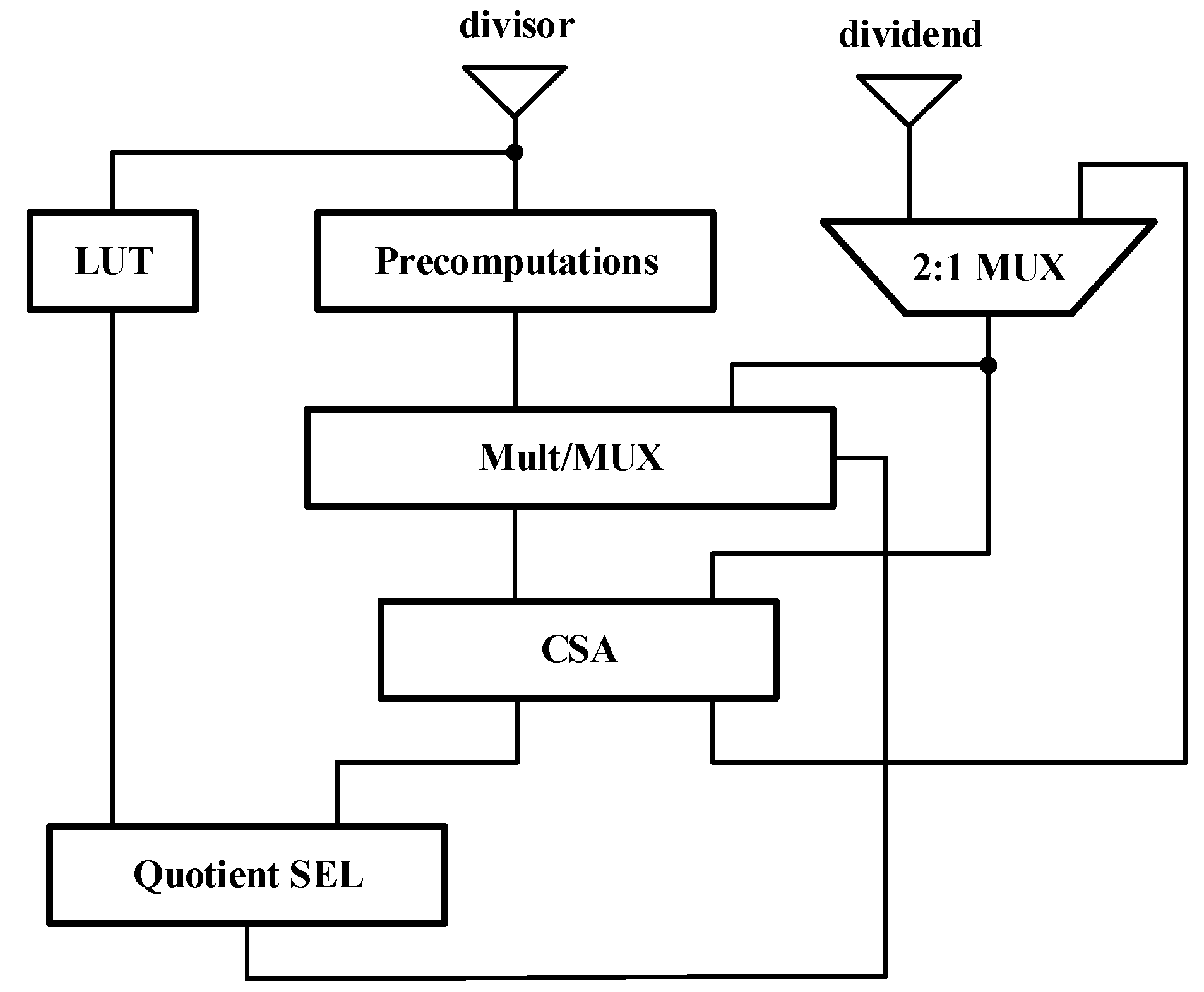
  25. Kasim, M.F.; Adiono, T.; Zakiy, M.F.; Fahreza, M. FPGA implementation of fixed-point divider using pre-computed values. Procedia Technol. 2013, 11, 206–211. [Google Scholar] [CrossRef] [Green Version]
  26. Oberman, S.F.; Flynn, M.J. Minimizing the complexity of SRT tables. IEEE Trans. Very Large Scale Integr. (VLSI) Syst. 1998, 6, 141–149. [Google Scholar] [CrossRef]
  27. Anane, M.; Bessalah, H.; Issad, M.; Anane, N.; Salhi, H. Higher Radix and Redundancy Factor for Floating Point SRT Division. IEEE Trans. Very Large Scale Integr. (VLSI) Syst. 2008, 16, 774–779. [Google Scholar] [CrossRef]
  28. Akkas, A. Dual-Mode Quadruple Precision Floating-Point Adder. In Proceedings of the 9th EUROMICRO Conference on Digital System Design (DSD’06), Cavtat, Croatia, 30 August–1 September 2006; pp. 211–220. [Google Scholar]
  29. Ozbilen, M.M.; Gok, M. Multi-Precision Floating-Point Adder. Ph.D. Thesis, Microelectronics and Electronics, Istanbul, Turkey, 2008; pp. 117–120. [Google Scholar]
  30. Jaiswal, M.K.; Cheung, R.C.C.; Balakrishnan, M.; Paul, K. Unified Architecture for Double/Two-Parallel Single Precision Floating Point Adder. IEEE Trans. Circuits Syst. II Express Briefs 2014, 61, 521–525. [Google Scholar] [CrossRef] [Green Version]
  31. Jaiswal, M.K.; Varma, B.S.C.; So, H.K.H. Architecture for Dual-Mode Quadruple Precision Floating Point Adder. In Proceedings of the 2015 IEEE Computer Society Annual Symposium on VLSI, Montpellier, France, 8–10 July 2015; pp. 249–254. [Google Scholar]
  32. Jaiswal, M.K.; Varma, B.S.C.; So, H.K.; Balakrishnan, M.; Paul, K.; Cheung, R.C.C. Configurable Architectures for Multi-Mode Floating Point Adders. IEEE Trans. Circuits Syst. I Regul. Pap. 2015, 62, 2079–2090. [Google Scholar] [CrossRef] [Green Version]
  33. Baluni, A.; Merchant, F.; Nandy, S.K.; Balakrishnan, S. A Fully Pipelined Modular Multiple Precision Floating Point Multiplier with Vector Support. In Proceedings of the 2011 International Symposium on Electronic System Design, Kochi, India, 19–21 December 2011; pp. 45–50. [Google Scholar]
  34. Manolopoulos, K.; Reisis, D.; Chouliaras, V.A. An efficient multiple precision floating-point multiplier. In Proceedings of the 2011 18th IEEE International Conference on Electronics, Circuits, and Systems, Beirut, Lebanon, 11–14 December 2011; pp. 153–156. [Google Scholar]
  35. Jaiswal, M.K.; So, H.K. Dual-mode double precision / two-parallel single precision floating point multiplier architecture. In Proceedings of the 2015 IFIP/IEEE International Conference on Very Large Scale Integration (VLSI-SoC), Daejeon, Korea, 5–7 October 2015; pp. 213–218. [Google Scholar]
  36. Akka¸s, A.; Schulte, M.J. Dual-mode floating-point multiplier architectures with parallel operations. J. Syst. Archit. 2006, 52, 549–562. [Google Scholar] [CrossRef]
  37. Bruguera, J.D. Radix-64 Floating-Point Divider. In Proceedings of the 2018 IEEE 25th Symposium on Computer Arithmetic (ARITH), Amherst, MA, USA, 25–27 June 2018; pp. 84–91. [Google Scholar]
  38. Saporito, A.; Recktenwald, M.; Jacobi, C.; Koch, G.; Berger, D.P.D.; Sonnelitter, R.J.; Walters, C.R.; Lee, J.S.; Lichtenau, C.; Mayer, U.; et al. Design of the IBM z15 microprocessor. IBM J. Res. Dev. 2020, 64, 7:1–7:18. [Google Scholar] [CrossRef]
  39. Burgess, N.; Williams, T. Choices of operand truncation in the SRT division algorithm. IEEE Trans. Comput. 1995, 44, 933–938. [Google Scholar] [CrossRef]
  40. Schwarz, E.M.; Flynn, M.J. Using a Floating-Point Multiplier’s Internals for High-Radix Division and Square Root; Tech. Rep. CSL-TR-93-554; Computer Systems Laboratory, Stanford University: Stanford, CA, USA, 1993. [Google Scholar]
  41. Pineiro, J.; Ercegovac, M.D.; Bruguera, J.D. High-radix iterative algorithm for powering computation. In Proceedings of the 2003 16th IEEE Symposium on Computer Arithmetic, Santiago de Compostela, Spain, 15–18 June 2003; pp. 204–211. [Google Scholar]
  42. Cortadella, J.; Lang, T. High-radix division and square-root with speculation. IEEE Trans. Comput. 1994, 43, 919–931. [Google Scholar] [CrossRef]
  43. Baesler, M.; Voigt, S.; Teufel, T. FPGA Implementations of Radix-10 Digit Recurrence Fixed-Point and Floating-Point Dividers. In Proceedings of the 2011 International Conference on Reconfigurable Computing and FPGAs, Cancun, Mexico, 30 November–2 December 2011; pp. 13–19. [Google Scholar]
  44. Chen, L.; Han, J.; Liu, W.; Montuschi, P.; Lombardi, F. Design, Evaluation and Application of Approximate High-Radix Dividers. IEEE Trans. Multi-Scale Comput. Syst. 2018, 4, 299–312. [Google Scholar] [CrossRef]
  45. Ercegovac, M.D.; Lang, T.; Montuschi, P. Very-high radix division with prescaling and selection by rounding. IEEE Trans. Comput. 1994, 43, 909–918. [Google Scholar] [CrossRef]
  46. Ercegovac, M.D.; McIlhenny, R. Design and FPGA implementation of radix-10 algorithm for division with limited precision primitives. In Proceedings of the 2008 42nd Asilomar Conference on Signals, Systems and Computers, Pacific Grove, CA, USA, 26–29 October 2008; pp. 762–766. [Google Scholar]
  47. Ercegovac, M.D.; McIlhenny, R. Design and FPGA implementation of radix-10 algorithm for square root with limited precision primitives. In Proceedings of the 2009 Conference Record of the Forty-Third Asilomar Conference on Signals, Systems and Computers, Pacific Grove, CA, USA, 1–4 November 2009; pp. 935–939. [Google Scholar]
  48. Vazquez, A.; Antelo, E.; Montuschi, P. A radix-10 SRT divider based on alternative BCD codings. In Proceedings of the 2007 25th International Conference on Computer Design, Lake Tahoe, CA, USA, 7–10 October 2007; pp. 280–287. [Google Scholar]
  49. Nannarelli, A. Radix-16 Combined Division and Square Root Unit. In Proceedings of the 2011 IEEE 20th Symposium on Computer Arithmetic, Tuebingen, Germany, 25–27 July 2011; pp. 169–176. [Google Scholar]
  50. Harris, D.L.; Oberman, S.F.; Horowitz, M.A. SRT division architectures and implementations. In Proceedings of the 13th IEEE Sympsoium on Computer Arithmetic, Asilomar, CA, USA, 6–9 July 1997; pp. 18–25. [Google Scholar]
  51. Carter, T.M.; Robertson, J.E. Radix-16 signed-digit division. IEEE Trans. Comput. 1990, 39, 1424–1433. [Google Scholar] [CrossRef]
  52. Atkins, D.E. Higher-radix division using estimates of the divisor and partial remainders. IEEE Trans. Comput. 1968, C-17, 925–934. [Google Scholar] [CrossRef]
  53. Chen, L.; Lombardi, F.; Montuschi, P.; Han, J.; Liu, W. Design of approximate high-radix dividers by inexact binary signed-digit addition. In Proceedings of the on Great Lakes Symposium on VLSI, Banff, AB, Canada, 10–12 May 2017; pp. 293–298. [Google Scholar]
  54. Nikmehr, H.; Phillips, B.; Lim, C. Fast Decimal Floating-Point Division. IEEE Trans. Very Large Scale Integr. (VLSI) Syst. 2006, 14, 951–961. [Google Scholar] [CrossRef] [Green Version]
  55. Tenca, A.F.; Ercegovac, M.D. On the design of high-radix online division for long precision. In Proceedings of the 14th IEEE Symposium on Computer Arithmetic, Adelaide, SA, Australia, 14–16 April 1999; pp. 44–51. [Google Scholar]
  56. Narendra, K.; Ahmed, S.; Kumar, S.; Asha, G.H. FPGA implementation of fixed point integer divider using iterative array structure. Int. J. Eng. Sci. Tech. Res. 2015, 3, 170–179. [Google Scholar]
  57. Jaiswal, M.K.; So, H.K. Architecture for quadruple precision floating point division with multi-precision support. In Proceedings of the 2016 IEEE 27th International Conference on Application-specific Systems, Architectures and Processors (ASAP), London, UK, 6–8 July 2016; pp. 239–240. [Google Scholar]
  58. Jaiswal, M.K.; So, H.K. Area-Efficient Architecture for Dual-Mode Double Precision Floating Point Division. IEEE Trans. Circuits Syst. I Regul. Pap. 2017, 64, 386–398. [Google Scholar] [CrossRef]
  59. Coke, J.; Baliga, H.; Cooray, N.; Gamsaragan, E.; Smith, P.; Yoon, K.; Abel, J.; Valles, A. Improvements in the Intels Cor2 Penryn processor family architecture and microarchitecture. Intel Technol. J. 2008, 12, 179–192. [Google Scholar]
  60. Gerwig, G.; Wetter, H.; Schwarz, E.M.; Haess, J. High performance floating-point unit with 116 bit wide divider. In Proceedings of the 2003 16th IEEE Symposium on Computer Arithmetic, Santiago de Compostela, Spain, 15–18 June 2003; pp. 87–94. [Google Scholar]
  61. Lichtenau, C.; Carlough, S.; Mueller, S.M. Quad precision floating point on the IBM z13TM. In Proceedings of the 2016 IEEE 23nd Symposium on Computer Arithmetic, Silicon Valley, CA, USA, 10–13 July 2016; pp. 87–94. [Google Scholar]
  62. Naini, A.; Dhablania, A. 1-GHz HAL SPARC64® dual floating-point unit with RAS features. In Proceedings of the 15th IEEE Symposium on Computer Arithmetic, Vail, CO, USA, 11–13 June 2001; pp. 173–183. [Google Scholar]
  63. Oberman, S.F. Floating point division and square root algorithms and implementation in the AMD-K7TM microprocessor. In Proceedings of the 14th IEEE Symposium on Computer Arithmetic, Adelaide, SA, Australia, 14–16 April 1999; pp. 106–115. [Google Scholar]
  64. Rupley, J.; King, J.; Quinnell, E.; Galloway, F.; Patton, K.; Seidel, P.M.; Dinh, J.; Bui, H.; Bhowmik, A. The floating-point unit of the Jaguar x86 Core. In Proceedings of the 2013 IEEE 21st Symposium on Computer Arithmetic, Austin, TX, USA, 7–10 April 2013; pp. 7–16. [Google Scholar]
Figure 1. Basic layout of very high-radix class algorithm.
Applsci 11 04988 g001
Figure 2. General architecture of the proposed division algorithm.
Applsci 11 04988 g002
Figure 3. The architecture of Exception Judgement module.
Applsci 11 04988 g003
Figure 4. The state transition diagram of Finite State Machine unit.
Applsci 11 04988 g004
Figure 5. The procedure of cycles in Finite State Machine unit.
Applsci 11 04988 g005
Figure 6. The architecture of Quotient Selection Unit module.
Applsci 11 04988 g006
Figure 7. The architecture of Partial Product Comparator module.
Applsci 11 04988 g007
Figure 8. The architecture of Product Comparator module.
Applsci 11 04988 g008
Figure 9. The architecture of Quotient Comparator module.
Applsci 11 04988 g009
Figure 10. Latency of the proposed FP division for SP, DP, and QP inputs.
Applsci 11 04988 g010
Table 1. Options of Parameter n.
Parameter nAdditional Digits of Quotient2n Kinds of Possible Quotients
112
224
338
4416
5532
Table 2. Different Patterns of Parameter m and t when n = 3 for Quadruple Precision FP division.
Parameter mParameter tData Width of LUT EntriesGuaranteed Bits per CycleClock CyclesAchieved Bits per Cycle
102512206 + 1 = 7120
103512294 + 2 = 6116
104512383 + 3 = 6114
1121024226 + 1 = 7132
1131024324 + 2 = 6128
1141024423 + 3 = 6126
1222048245 + 1 = 6120
1232048354 + 2 = 6140
1242048463 + 3 = 6138
Table 3. Judgement for Exception Signal.
Input DividendInput DivisorException Signal Exception
NaNNaNNaN
NaNZeroNaN
NaNInfinityNaN
ZeroNaNNaN
ZeroZeroNaN
ZeroInfinityZero
InfinityNaNNaN
InfinityZeroNaN
InfinityInfinityNaN
Table 4. ASIC Implementation Details @ TSMC 90 nm.
SPDPQP
Latency(cycle)346
Period(ns)3.33.33.3
Total time(ns)9.913.219.8
Efficient average time (ns/bit) 10.430.250.17
Area(μm2)542,650545,905550,567
Power(mW)55.5856.1358.53
1 Efficient Length refers to mantissa length of relevant precision: 23 for SP, 52 for DP, and 112 for QP.
Table 5. Comparison of Predict–Correct Division Architecture On DP.
[58] (with 1-Stage Multiplier)[58] (with 2-Stage Multiplier)This Paper
Subnormal
Tech.90 nm90 nm90 nm
Latency (cycle)11 (61.1%)18 (100%)4 (22.2%)
Period (ns)1.72 (175.5%)0.98 (100%)3.3 (336.7%)
Power (mW)30.9 (48.1%)64.21 (100%)58.53 (91.1%)
Total time (ns)18.92 (107.3%)17.64 (100%)13.2 (74.82%)
Total energy (fJ)584.65 (51.6%)1132.74 (100%)772.6 (68.2%)
Efficient average energy (fJ/bit) 111.24 (51.6%)21.78 (100%)12.07 (55.4%)
1 Efficient Length in Table 5 equals to 52 for DP.
Table 6. Division Latency Comparison.
AlgorithmTech.Clock Speed (Hz)SPDP
Latency (Cycle)Total Time (ns)Latency (Cycle)Total Time (ns)
AMD K7multiplicative500 M16322040
AMD Jaguarmultiplicative28 nm2 G147199.5
IBM zSeriesradix-4130 nm1 G23233737
IBM z13radix-8/422 nm5 G183.6285.6
HAL Sparcmultiplicative150 nm1 G16161919
Intel Penrynradix-1645 nm2.33 G125.14208.57
This paperPredict–Correct90 nm300 M39.9413.2
Publisher’s Note: MDPI stays neutral with regard to jurisdictional claims in published maps and institutional affiliations.

