1. Introduction
The building industry, as an important basic industry of the national economy, has a pivotal role in improving human settlements, managing the ecological environment, and developing a circular economy [
1]. At the same time, the construction industry, along with power generation and automobile use, is one of the three major sources of greenhouse gas emissions threatening the Earth’s climate [
2]. Today, buildings still account for nearly 40% of global energy consumption and carbon emissions [
3,
4]. Governments around the world are adopting and implementing various financial regulations and incentives to mitigate the impact of the built environment [
5].
The International Organization for Standardization and the International Society for Environmental Toxicology and Chemistry have defined a life cycle impact assessment framework and a list of life cycle impact parameters with 18 categories [
6]. The Product Social Impact Life Cycle Assessment database version 1.0 summarizes data from about 15,000 departments and 189 countries/regions around the world, and finally determines 88 qualitative and quantitative indicators [
7]. Researchers use midpoint and endpoint modelling in the full life cycle feature modelling and weight factor analysis. The weighted parameters for influencing factors are optimized by Monte Carlo simulation set by software after empirical setting [
8,
9]. No scientific research methods have been established to improve the reliability and accuracy of influencing parameters.
After analyzing the above research, some ideas appear: whether the software evaluation criteria are consistent [
10,
11], whether the database is updated in time, whether the case analysis is perfect [
12], whether the theoretical modelling is more practical [
13], and whether the special research on complex structure bridges and the environmental, economic, and social impacts of the project are considered [
14].
The goal of the research is to meet the maximum safety and minimum life cycle cost and environmental impact in order to solve the above-mentioned problems [
15]. The first problem is to improve the reference framework and method of bridge life cycle assessment.
This work solves the following problems:
① A Bayesian network fuzzy mathematical model is established to solve the uncertainty problem of the environmental impact factors of bridges.
② The conclusion of the software analysis is checked to improve the accuracy and refinement of the research.
③ In order to provide research ideas for reducing environmental pollution, the database optimization analysis is carried out in the stage of environmental contribution.
④ Research has proved that basic science and applied science are closely related [
16], and that strong theoretical support requires sufficient calculations for testing.
Through the establishment of the BNFC model, the environmental impact weight of five stages is deduced and calculated. The environmental impact of bridge is analyzed by OpenLCA software.
The innovation of this work lies in the application of BN and FMT in the process of the environmental impact assessment of bridges. First, the uncertain multi-factors are modelled and scientifically calculated. The calculation conclusion is applied to the analysis and evaluation process of the LCA software again, and finally the analysis conclusion is fitted with the modelling calculation, and the two are linearly consistent. We realize the accurate processing and effective evaluation and comprehensive analysis of uncertain data in the LCA evaluation process, and improve the accuracy of uncertain factors in LCA analysis.
2. Literature Review
2.1. Current Situation of Research Results on Environmental Impact of Construction Industry
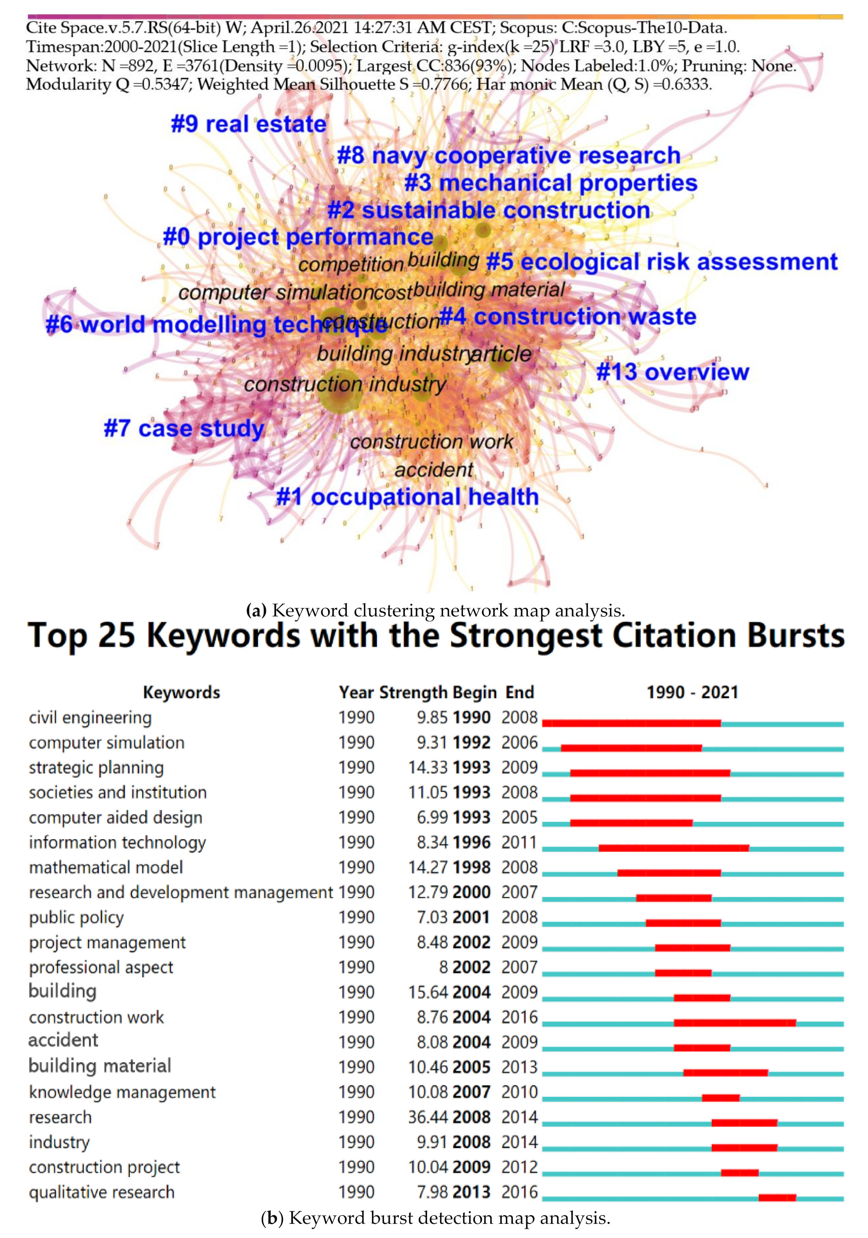
The research group searched the publishing results related to the three keywords of construction industry, environment, and research through Scopus [
17], and found a total of 5391 articles and conference literature (1990–2021). This paper selects the journals published from 1990 to 2020 (accounting for 93.26% of the total articles) for cluster statistical analysis, as shown in
Figure 1.
The survey results show that the environmental impact research results of the construction industry are increasing year by year, with the increasing rate reaching 11.36%; the growth rate of global environmental impact research regions is 4.83%, with the total number reaching 104 countries and regions, accounting for 44.64% of the global total [
18]. The number of publications in the top ten countries accounted for 87.40% of the total, while other countries and regions only accounted for 12.6%. Therefore, environmental governance has nothing to do with political, economic, and cultural background [
19].
Cluster analysis of articles published globally over 31 years showed that the core words project performance, occupational health, sustainable construction, etc. ranked as the top ten words that are not related to mathematics. Articles about mathematical theoretical models appeared during the period of 1998–2008, and the combination of environment and mathematical modelling theory was missing. There is a phenomenon of interdisciplinarity between clusters. After 2008, the number of articles being published decreased, but the research direction broadened systematically and comprehensively, and it tended to focus on environmental sustainability. Researchers now pay more attention to systematic research on environmental impact. The analysis conclusions show that basic science and form science are developing simultaneously, and interdisciplinary applications are necessary. Multidisciplinary research can reduce the uncertainty in the software analysis process, further improve the accuracy of Monte Carlo simulation, and make the research more complete and more scientific.
2.2. Uncertainty of Environmental Impact Factors in Construction Industry
The construction industry provides the necessary infrastructure and buildings for human activities [
20], while emitting 33% of the global carbon [
21]. According to industry standards, it can be divided into direct and indirect emissions [
22]. Direct emissions refer to carbon emissions generated in design, construction, maintenance, and demolition activities [
23,
24]; indirect emissions refer to the industrial upstream activities of all raw materials [
25]; therefore, it is difficult to conduct a comprehensive evaluation on the micro level [
26]. Macroscopically, the construction industry has close interaction with other industries [
27]. How can we accurately capture the dynamic influencing factors in the whole project life cycle [
28], how do we accurately study the discrete state of engineering uncertain factors is the key [
29,
30], and how do we judge and ignore the uncertain influencing factors for accurate modelling [
31]? This is also a problem to be solved in this work. Accurately determining the uncertainty of influencing factors can improve the analytical value of research data at each stage and the optimization of database-related data, while excluding empirical assumptions and speculations.
2.3. Environmental Impact Assessment Method of Construction Industry
Considering the uncertainty of data in LCA analysis of bridges, Monte Carlo simulation and genetic algorithm are widely used [
32,
33]. Researchers proved the sustainability of LCA by weighting the analytic hierarchy process and assessment [
34,
35]. Sánchez-Garrido and Yepes used multi-criteria assessment to optimize villa sustainability [
36].
In view of the diversification of LCA research software and research methods and the differences between them, the research team decided to expand the search scope and research scope in Scopus. The key words included: environment, engineering, bridge, and research method. In total, 2624 articles and conference papers were retrieved. From 2010 to 2021, 1447 articles were classified according to 160 keywords, and the analysis methods used included: the finite element method (251), Monte Carlo methods (71), numerical model (333), neural networks (98), genetic algorithms (77), and sensitivity analysis (134). No more specific and effective strategies were found for the uncertain factors in LCA.
Openlca1.10 [
37] was used in this research. The software uses Monte Carlo simulation to perform uncertainty distribution and geometric mean and geometric standard deviation [
11]. Before the software system started the simulation, it was necessary to empirically set the influence weight coefficient of each influencing parameter. The question arises: does every researcher have rich engineering construction management experience? If researchers without similar architectural experience have determined the impact weights, are the research conclusions perfect and accurate, and how do we solve this problem scientifically?
2.4. Determination of Environmental Impact Assessment Method
How do we accurately reflect the change characteristics of a dynamic environment and update parameters [
38], and how can we qualitatively and quantitatively describe the dependence between variables using the proposed Bayesian Networks [
39]. A Bayesian network is an effective tool for probabilistic modelling and causal reasoning, which is effective for reliability modelling and evaluation of complex systems under dynamic conditions [
40].
In the field of construction engineering, it is difficult to obtain accurate probability values [
41]. Fuzzy set theory is usually used to deal with fuzzy and imprecise events effectively [
42], and fuzzy mathematics theory is introduced. Fuzzy mathematics theory and Bayesian networks are both powerful and effective tools for knowledge reasoning in uncertain environment [
43,
44]. Therefore, in this work, FMT and BN are used as a decision-making method, referred to as BNFC. BNFC solves the problems in the above analysis and further improves the feasibility and scientific of the research. This model improves the effective evaluation and dynamic processing of uncertain factors in LCA research.
3. Methodology
3.1. Research Theory (BN and Basic Principles of FMT)
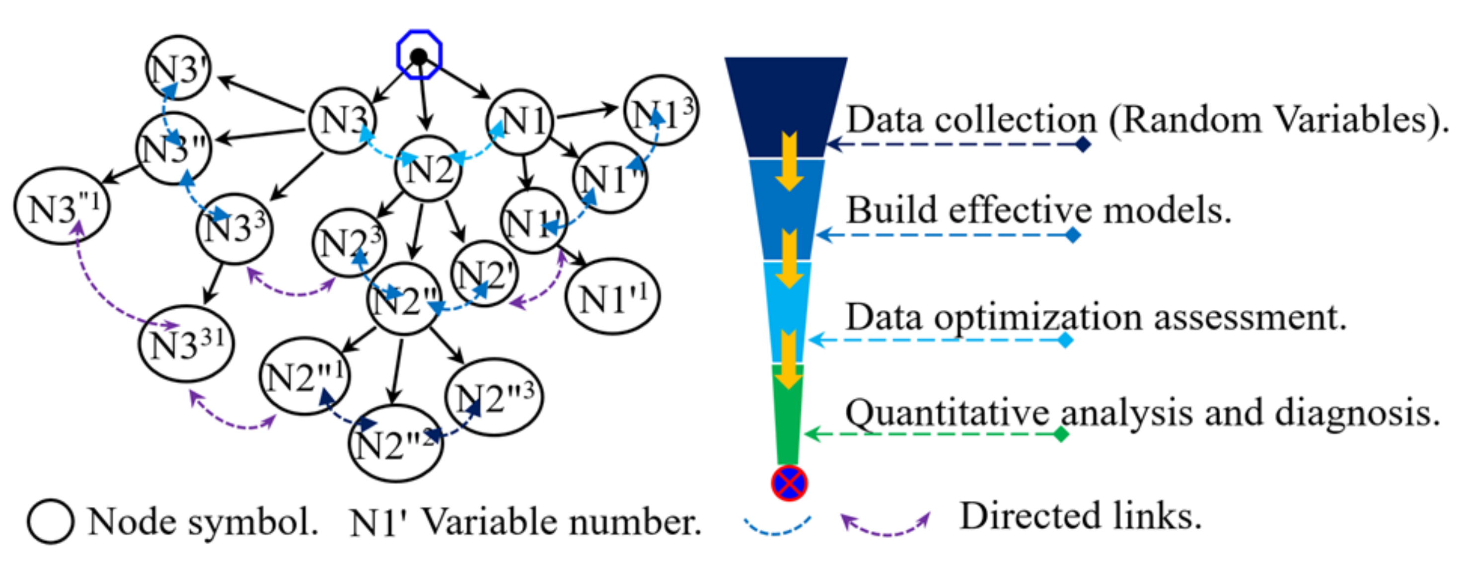
As shown in
Figure 2, as the complexity of influencing factors increases, the diversity and uncertainty of parameters increase. How do we properly model and quantify to improve the reliability of data [
45]? Bayesian network is a system modelling language used to deal with the relationship between random variables [
46], in order to achieve the best accurate reasoning conclusion [
47].
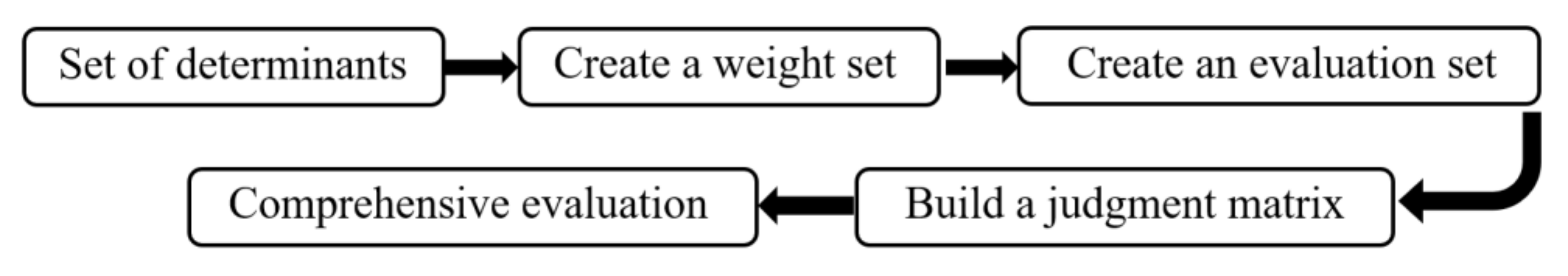
In 1965, Zadeh, L.A., an American cybernetic scholar, first proposed the concept of “Fuzzy Mathematics”. A new fuzzy set and membership frame model is proposed to solve and deal with the inaccuracy of information representation and reasoning [
48]. Fuzzy mathematics is a mathematical theory and method to study and deal with fuzzy phenomena (
Figure 3). Through the analysis of fuzzy comprehensive evaluation, we can find out the common rules and attributes of set objects and establish the model [
49].
3.2. Theoretical Model Bridge Process
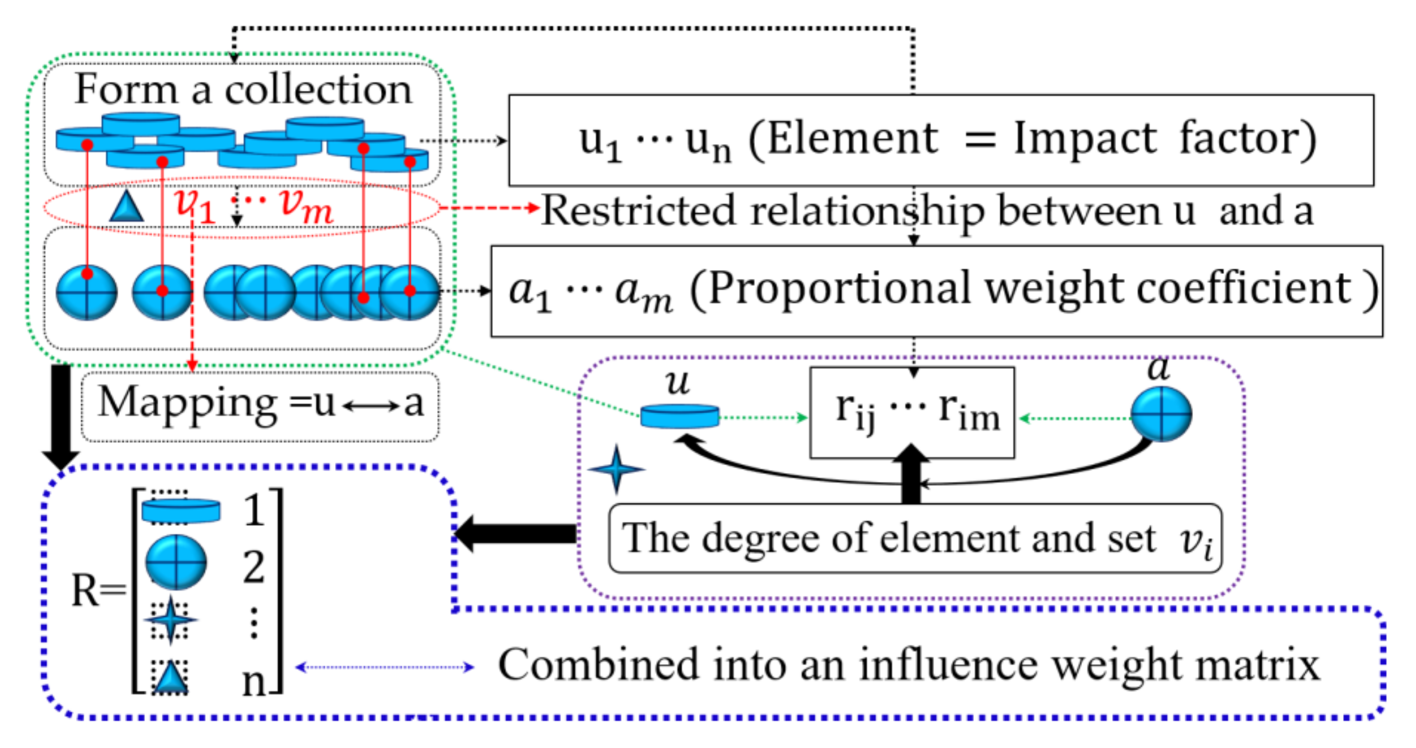
The introduction of some important definitions used in FMT structural hierarchy theory helps to fully understand the subsequent modelling applications (a single factor influences the weight matrix: the FMT comprehensive evaluation principle is based on the analysis and evaluation of each single impact factor (
) in
, and after the analysis is completed, it is summarized into a set form (
Figure 4). To solve the maximum eigenvalue
and corresponding eigenvector
of the judgement matrix at this level, the judgement matrix needs to be normalized as the impact factor of this level on the previous level.
Consistency index:
where
is the consistency index;
is the maximum eigenvalue of the judgement matrix; and
is the number of levels.
where
is the consistency ratio; and
is the average consistency index.
Equation (1) is substituted into Equation (2), giving
Judgement basis: if ≥ 0.1, the consistency of the impact weight matrix is not acceptable; if < 0.1, the consistency of the impact weight matrix is acceptable.
Hypothesis set
=
, weight set
=
, and comment set
=
are established according to the fuzzy synthetical assessment theory. To perform quantitative results analysis, the comment set is divided into five levels, as shown in
Figure 5:
Description: There are a total of 117 environmental impact factors for cable-stayed bridges. The amount of data information is huge—see the attached table for relevant data.
The
-th impact factor is evaluated by the
the factor
of the assessment object (factors at each phase), and the degree of membership of the
th element
in the comment set is
(∈
∉ cannot be used) because the fuzzy set has no strict demarcation. The degree of membership, that is,
, is introduced to represent the degree of belonging of the element
to the fuzzy set
[
50];
is any number between 0 and 1. The fuzzy set
of factors
can be expressed as:
where
is the assessment set of a single factor;
is the membership of
kinds of elements; and
is the comment set of
kinds of elements. All the single-factor fuzzy assessment sets are integrated into an impact weight matrix:
where
is the single-factor fuzzy impact weight matrix.
3.3. LCA Research Framework and Parameters
ISO stipulates the LCA standard research framework: the goal and scope definition, inventory analysis, impact assessment, and interpretation. These are GWP, AP, FEP, PMFP and WP. It includes five stages: survey and design, material manufacturing, construction and installation, maintenance and operation, and disassembly and recycling [
11]. OpenLCA1.10 software is the analysis software used in this study [
37]. The databases used in this study include Ecoinvent [
51] and Bedec [
52].
3.4. Research External Conditions
We followed the regulations and research results of the United Nations Environment Programme (UNEP); the Joint Research Center of the European Commission and Mansour Rahimi and others and have reconsidered the use of research methods [
53,
54,
55].
In consideration of the above representative research results and 2.1 and 2.2, the BNFC was combined with the midpoint and the endpoint to build a model. We chose sufficient raw data and effective evaluation. The focus was on traffic pollution during the maintenance phase.
3.5. Impact Factor
In the study by Zhou et al., according to the characteristics of the full life cycle of the cable-stayed bridge, the value of the influence factor of each stage was accurately defined, which laid the foundation for the analysis conclusion [
11]. The analysis in OpenLCA1.10 software needs to set the range of influence factors (1.00 to 1.50) at each stage. In this study, a more accurate BNFC was used to synthesize weighted impact factors.
3.5.1. Bridge a BN Hierarchical Analysis Model
Figure 5 shows the five levels of impact index analysis and assessment built based on research results and the BN. The first level is the total contribution of the cable-stayed bridge to environmental emissions; the second level is the values of the five stages; the third level is the value of the contribution of each process; the fourth level is the value of the contribution of each type; and the bottom level is the values of the contributions of materials and equipment.
3.5.2. Establishing Impact Weight Matrix
The comprehensive assessment of impact factors is considered in the bridge analysis. The fuzzy comprehensive assessment hypothesis is expressed as
=
=
, where
is the fuzzy composition operator; and
is the fuzzy comprehensive assessment index. An equation can be obtained as follows based on the generalized fuzzy operations
where
= (1, 2,
, Λ,
);
represents the operation “or”; and
represents the operation “and”.
The comprehensive Bayesian fuzzy impact weight model can be written as:
3.5.3. Hypothesis
As shown in
Figure 5, there is 1 first-level indicator, 5 second-level indicators, 31 third-level indicators, 68 fourth-level indicators, and 12 fifth-level indicators to derive the conclusion based on Equations (1)–(5).
= 0, . The interval range of the influence factor is calculated by taking the value of , combining the eigenvectors of each stage and the preliminary assumption of the interval range set by the LCA software. We can assume the impact factor weight parameters as being = (1.00, 1.02, 1.10, 1.45, 1.01). The conclusions of analyses of subsequent cases will be used to check the accuracy of the assumed weight parameters.
4. Case and Results
4.1. Case Description
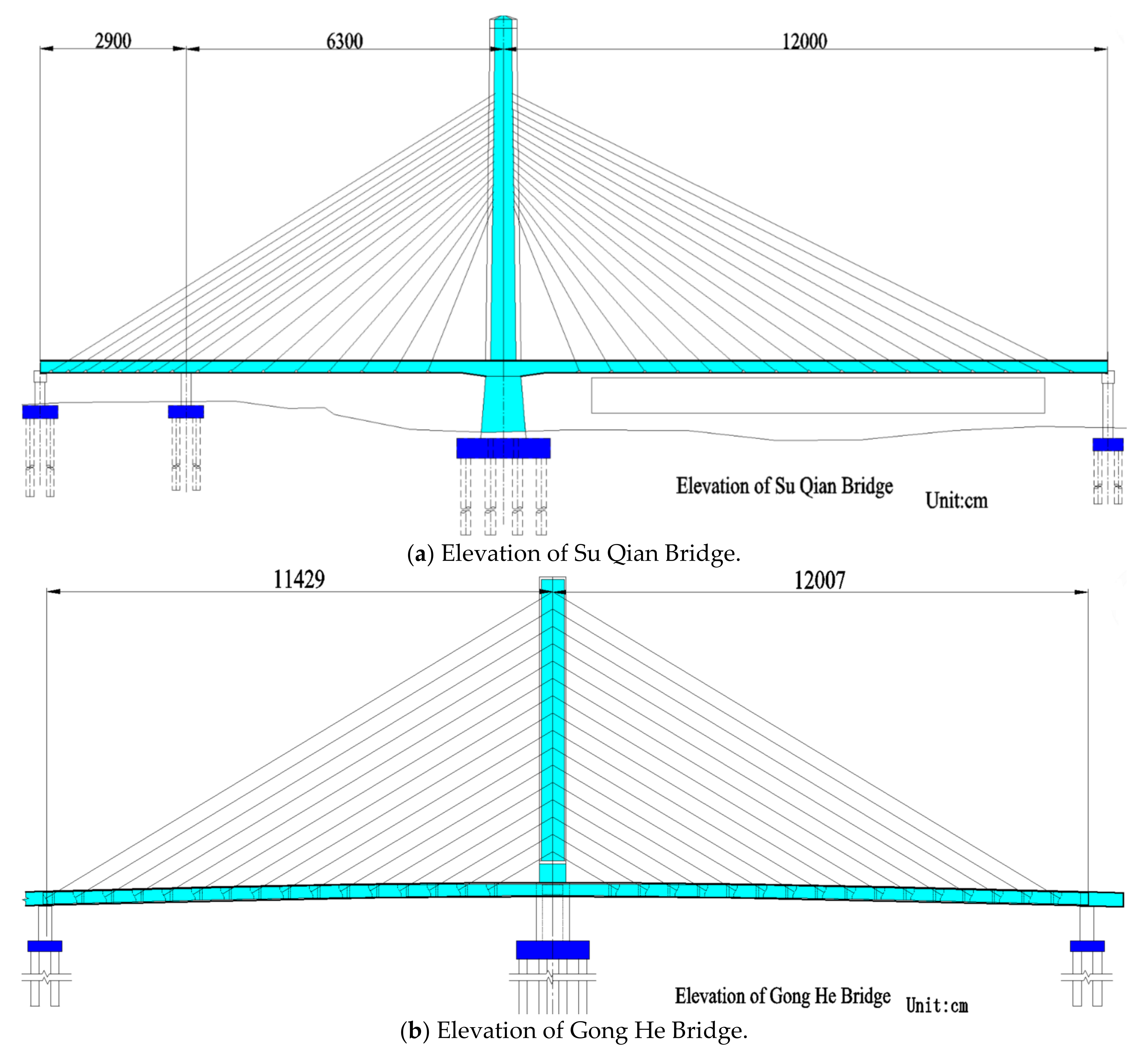
To better apply fuzzy mathematics to study the uncertain data of bridges, careful comparison and consideration have been made in the selection of bridge cases: bridges have similar structural types (cable-stayed bridges), similar lengths, the same construction schemes, and the same purpose (first-class highway bridge), and the designed lifetime is 100 years.
Case 1: SQ is a canal bridge. The main bridge has a total length of 212 m, a width of 26.5 m, a beam height of 2.3 m.
Figure 6 shows C cable-stayed bridge. The main tower is built using a creeping formwork. The side span beam and the girder #0 are cast in place with the bracket method, and girders #1~#16 are constructed with a hanging basket [
56].
Case 2: EH is in the Lao Dao Kou area of Shenyang, China. The main bridge is a cable-stayed bridge, with a span of 236 m, a width of 32 m, and a beam height of 3.16 m. The top plate of the beam is 26 cm thick, the bottom plate is 24 cm thick, as
Figure 6 shows. The beam blocks #1~#13 (−#1~−#13, with #1~#16 on the left and −#1~−#16 on the right.) are built using the slide formwork method, and blocks #0 and #14~#16 (−#14~−#16) are built using the cast-in-place method [
57].
The contributions of the two cable-stayed bridges to environmental emissions in five phases are analyzed first, as shown in
Figure 5. Data sources include design contracts and plans, data from the survey and design phase, construction drawings, geological survey reports, construction organization design, published research results, observed local transportation data, observation data obtained from environmental protection and meteorological departments, and the Ecoinvent and Bedec databases. The criteria for the use of research resources include rich experience in bridge engineering, scientific research theories, and comprehensive research and analysis capabilities.
According to the LCA analysis process, the energy consumption of the bridge occurs in five stages, mainly in the material manufacturing stage and the maintenance and operation stage.
4.2. Survey and Design
The pile foundations of SQ and EH are end bearing piles. According to China (GB) 50021-2001 regulations [
58], the distance between exploratory points of end bearing piles is 12~24 m and the distance between exploratory points of friction piles is 20~35 m; the depth of exploration is expected to increase by 3~5 m. See
Table 1 for specific data.
4.3. Material Manufacturing
The main materials of SQ and EH are C (C50, C40, C30, C25, C20, C15), asphalt C, steel bars, steel strands, profiles, bellows, anchors, cables, and so on. Auxiliary materials include one creeping formwork for each tower (the weights of the creeping formworks of SQ and EH are 28.2 and 32.2 tonnes, respectively) and one hanging basket for SQ’s girder, with a weight of 210 tonnes. EH’s girder uses a slide formwork (the entire system consists of a formwork, fixed pier and mounting bracket, traction and slide devices, rear hanging equipment, etc.) with a weight of 360.67 tonnes.
Sections #0 and−#16~−#7 of SQ adopt the bracket method (the bracket pipe should have a wall thickness of 3.0 mm and a diameter of 48 mm) for cast-in-place construction. The length is 76.5 m, the average height is 12 m, and the weight is 2770.72 tonnes. Sections #0 and #14~#16(−#14~−#16) of EH adopt the bracket method (the bracket pipe should have a wall thickness of 3.0 mm and a diameter of 48 mm) for cast-in-place construction. The length is 66 m, the average height is 7 m, and the weight is 1552.78 tonnes.
Both bridges are municipal projects and use commercial C according to the contract. The transportation distances from SQ and EH to the commercial C plant are 16 and 15 km, respectively.
4.4. Construction and Installation
The main processes of SQ are the construction of main piers and foundations; the construction of side piers, auxiliary foundations, and foundations; the erection of bracket #0 and construction of the lower tower column and block #0 of the main tower; the construction of the upper tower of the main tower and erection of side span cast-in-place bracket; the installation of the hanging basket and repeat pouring of blocks #1~#16(–#1~−#16); the cast-in-place construction of the side span; the locking of the closure section; and the bridge floor and auxiliary construction.
The main processes of EH are the pile foundation construction; bearing platform construction; pier body construction; the cast-in-place #0 block after erecting the steel pipe support; the pouring construction of the main tower’s creeping formwork; the hanging of cable #1; the installation of the hanging basket; the guide cable construction before the cable-stayed basket; the pouring of blocks −#1~−#13 and #1~#13; the pouring of blocks −#14, −#15 and #14, #15, and #16 on the bracket; drawing girders together; stretching the anchor bolts; and paving the bridge deck.
The construction of side piers involves the construction of the side pier pile foundation, bearing platform, and pier body, pouring of blocks −#14, −#15, #14, #15, and #16 by the bracket method, leaving 1.5 m at the end of block #14 as the closure section, and casting the C at the closure section by hanging formworks on both sides. See
Table 2 for specific data.
4.5. Operation and Maintenance
According to the design codes for bridges and culverts in China (JTJ021-89, 024-85, 023-85, 004-89), the service life of a cable-stayed bridge is 100 years. To ensure the safety and normal use of the bridge during the design reference period, the maintenance department should carry out regular maintenance and repair. The maintenance cycle is shown in
Table 3.
The existing carbonization models are basically divided into four categories: theoretical models [
59], empirical models [
60], semi-theoretical and semi-empirical models [
61], and random models [
62].
The theoretical model of carbonization depth can be simplified as:
where X is the carbonization depth; t is the carbonation reaction time; and k is the carbonation coefficient (A comprehensive parameter reflecting the rate of carbonization).
The China promulgated GB/T51355-2019 in 2019 stipulates that the calculation formula of C carbonization coefficient is [
63]:
where
is the carbonation coefficient of C (mm/
);
is the influence coefficient of CO
2 concentration, which is set as
—CO
2 concentration;
is the CO
2 concentration (%);
is the location influence coefficient (1.4 or 1.0);
is the
casting surface influence coefficient, and is set up 1.2;
is the working stress influence coefficient, which is set as 1.0 in the compressive zone and as 1.1 in the tensile zone;
is the environmental temperature (℃);
is the environmental relative humidity;
is the substitution coefficient of fly ash; and
is the extrapolated value of C compression strength (MPa).
Yu et al. determined the model relationship of CO
2 absorption capacity per unit volume of concrete [
64].
where
is the CO
2 absorption capacity of ordinary Portland cement (mol/m
3);
is the number of cementitious materials used per unit volume of
(kg/m
3); and α is the number of mixed materials in ordinary Portland cement (%).
The carbonization of SQ and EH is judged and analysed in accordance with (8), (9) and (10).
4.6. Disassembly and Recycling
Each year, the global C industry generates more than 11 billion tonnes of waste, of which C waste accounts for about 50–70% [
65]. According to a study by [
66], the recycling rates of aggregates in Norway and China are 30 and 7%, respectively. It is necessary to manage construction waste in a sustainable way [
67,
68]. In view of reducing the environmental pollution of construction waste and the value of China’s waste recovery rate, combined with the urban location of the two bridges. The comprehensive analysis will be through mechanical and manual dismantling, and then sustainable recycling after 100 years of operation.
The demolition period of SQ and EH is 65 days and 75 days, respectively. There are 26 and 32 construction personnel, respectively. Demolition waste is transported to a steel plant 330 km (58 km) away and a waste-to-energy plant 846 km (52 km) away.
5. Discussion
The five phases of the bridge will produce environmental pollution, and improving sustainable development is the best choice to reduce pollution [
69,
70,
71] (Intergovernmental Panel on Climate Change).
Table 4 shows the framework and modelling formulas of the contributions of the five phases of a cable-stayed bridge to environmental emissions. The contribution to environmental emissions of secondary use is mainly caused by the steel recycling and refining. After the bridge is dismantled by the mechanical crusher, the loaders will be used for on-site sorting and loading. This increases the steel recycling rate to 90% [
72] and the C scrap recycling rate to 55% [
73]. The remaining construction wastes are transported to garbage power plants and landfills for disposal. There is no garbage power plant in the surrounding area of SQ, and all the remaining construction wastes are transported to landfill for disposal.
5.1. Case Environmental Impact
5.1.1. BNFC Comprehensive Assessment
According to the results of the LCA study, the total environmental emissions contributions of SQ and EH are 147,446.95 and 135,311.42 tonnes, respectively, as shown in
Table 5. Among the five contribution values, the GWPs of SQ and EH account for 95.67% and 95.47%, respectively.
GWP, AP, FEP, PMFD, and WP were selected as assessment factors to build the grading system for each phase. According to the theory presented in
Section 3.3.
where
is the survey and design stage;
is the material manufacturing stage;
is the construction and installation stage;
is the maintenance and operation stage; and
is the disassembly and recycling stage.
The fuzzy matrix was established as follows according to
Table 6 and Equation (5):
and
and
were determined according to Equations (6) and (7), as shown in
Table 7.
The assessment result can be obtained as follows by the compound operation
=
:
5.1.2. Comparative Analysis of the Results of Fuzzy Comprehensive Assessment of LCA and Bayesian
According to the conclusion of the assessment in
Section 5.1.1 and the results of software analysis shown in
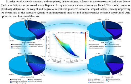
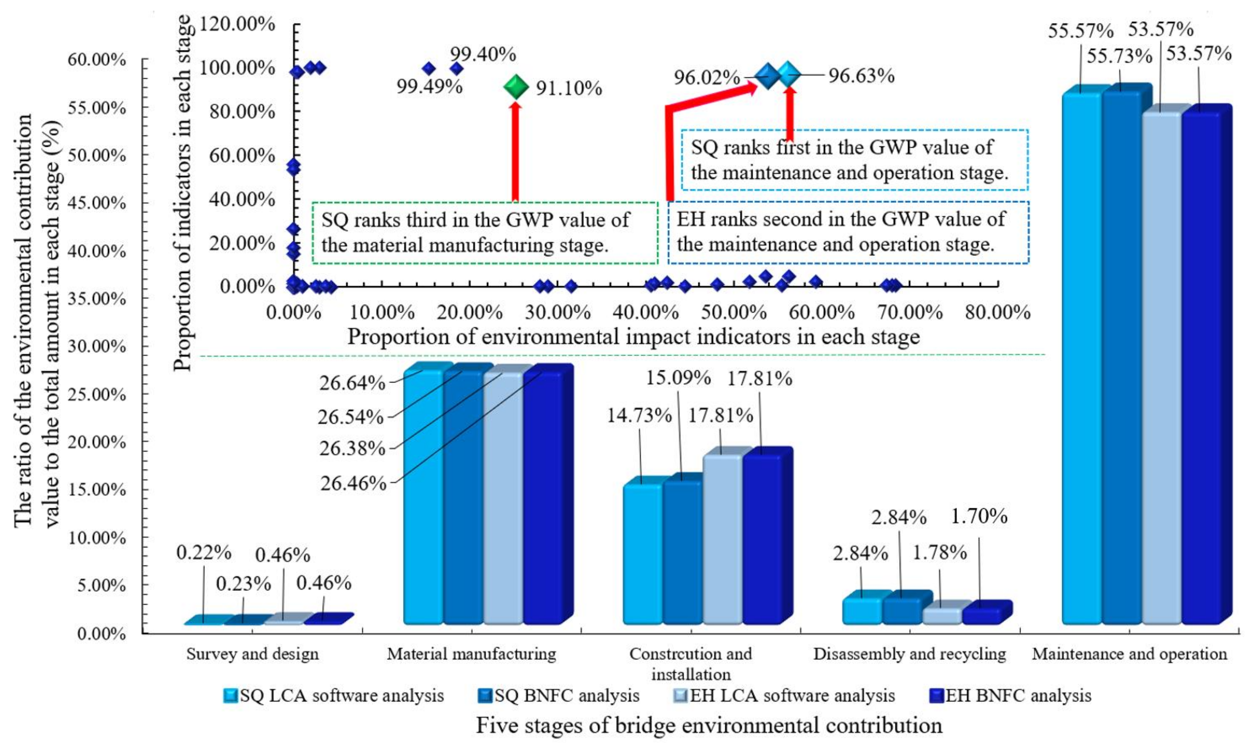
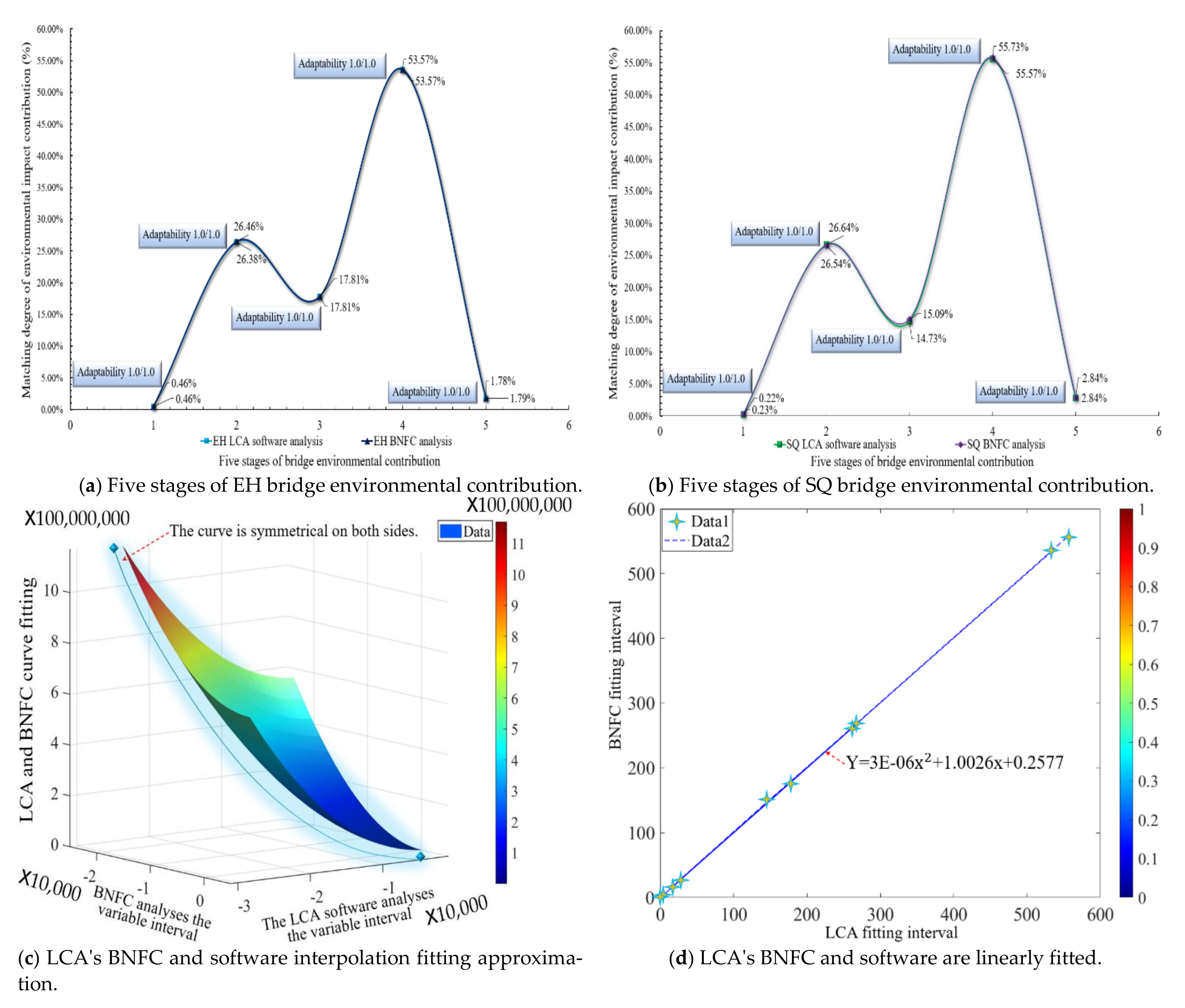
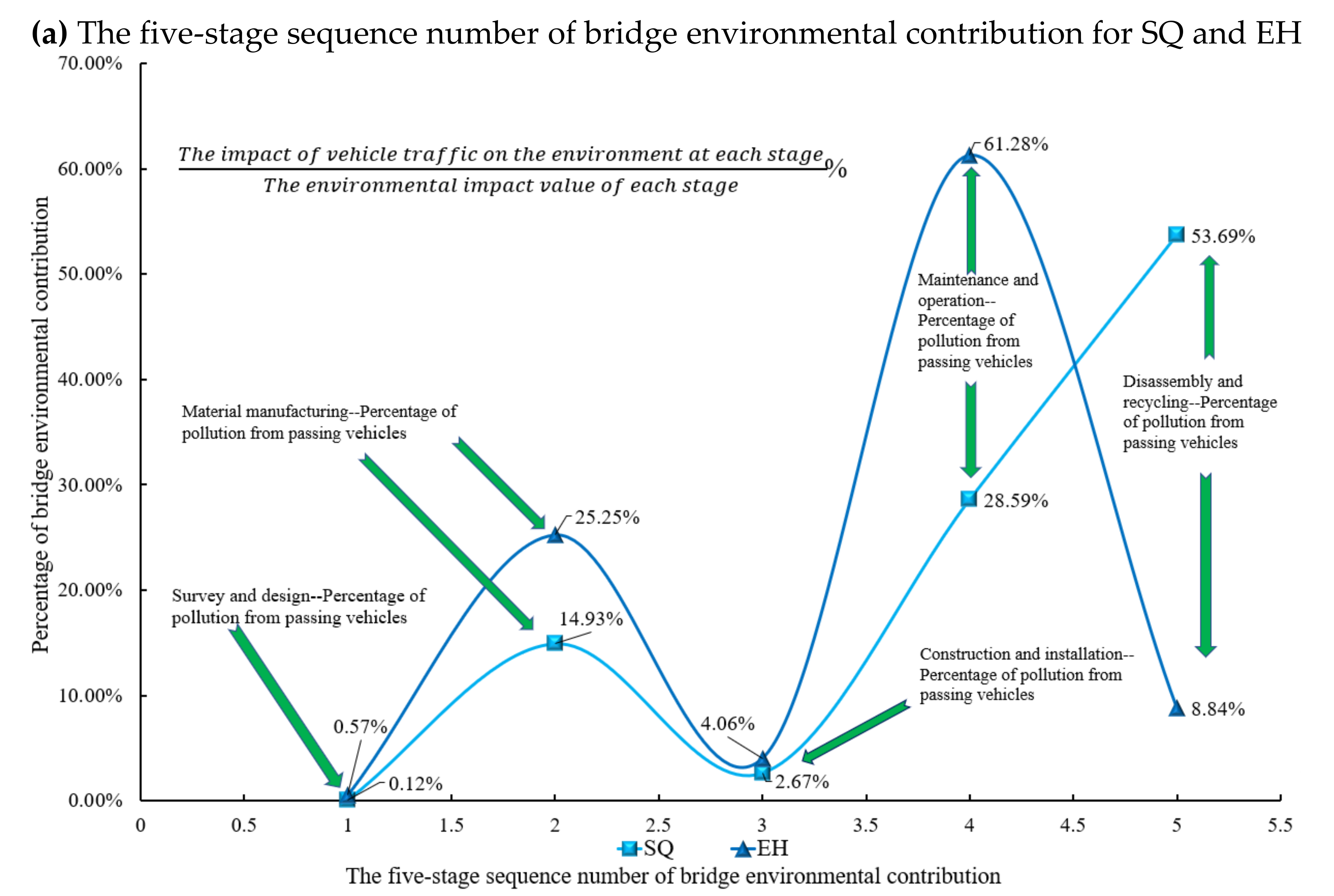
Figure 7, the contributions to environmental emissions of SQ according to the software analysis can be ranked from high to low as follows: operation and maintenance (55.57%) > material manufacturing (26.64%) > construction and installation (14.73%) > disassembly and recycling (2.84 %) > survey and design (0.22%), and SQ’s contributions according to the BNFC can be ranked from high to low as follows: maintenance and operation (55.73%) > material manufacturing (26.54%) > construction and installation (15.09%) > disassembly and recycling (2.84%) > survey and design (0.23%).
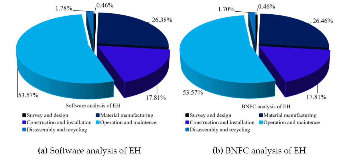
As shown in
Figure 8, the contribution to environmental emissions of EH according to the software analysis can be ranked from high to low as follows: maintenance and operation (53.57%) > material manufacturing (26.38%) > construction and installation (17.81%) > disassembly and recycling (1.78%) > survey and design (0.46%), and EH’s contribution according to the BNFC can be ranked from high to low as follows: maintenance and operation (53.57%) > material manufacturing (26.46%) > construction and installation (17.81%) > disassembly and recycling (1.70%) > survey and design (0.46%).
Figure 9 shows that the conclusions obtained by the application software are basically consistent with those obtained by BNFC. For the maintenance and operation phase and the construction and installation phase of SQ, the differences between the results of the two approaches are 55.57%–55.73% = –0.16% and 14.73%–15.09% = –0.36%. For the material manufacturing phase and the disassembly and recycling phase of EH, the differences between the results of the two research conclusions are 26.38%–26.46% = –0.08%, and 1.78%–1.70% = –0.08%. Other data are basically the same. Therefore, it is determined that the conclusions for SQ and EH obtained by the two research methods are both accurate.
We applied the Matlab scientific computing programming method to the above conclusions to calculate the conclusion fitting (shown in
Figure 10). The research image and the fitted data show that there is no discrete type of data between the software analysis results and the BNFC analysis conclusions, and the data are completely symmetric and matched. The fitted quadratic curve is
, and the linearity tends to a straight line, indicating that the two research methods are very consistent.
5.1.3. Impact Factor Calibration for SQ and EH
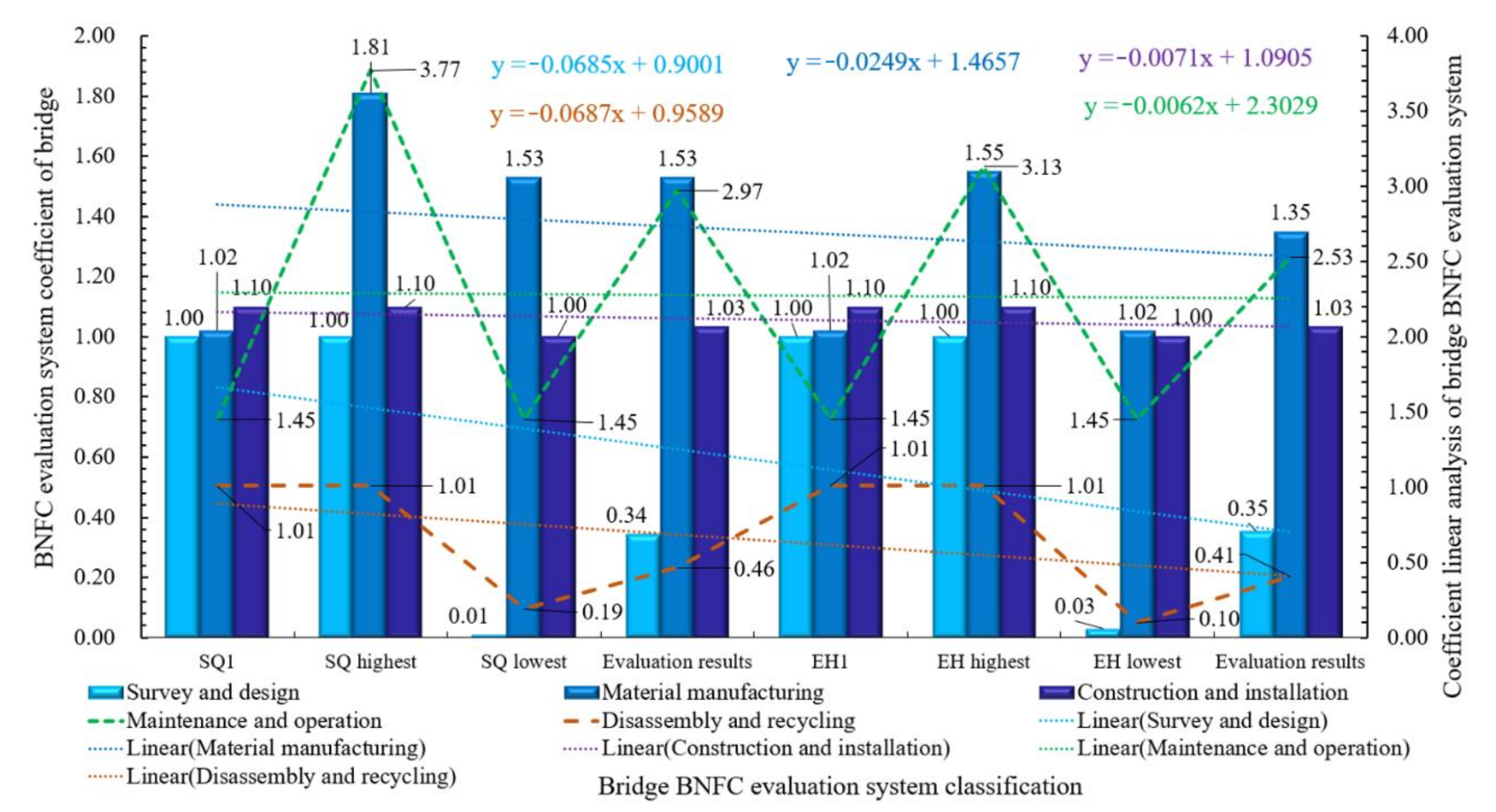
The impact factors of SQ and EH are obtained after the analysis by means of the BNFC analytic hierarchy process.
Table 5 shows the results of the LCA analysis, and
Section 5.1.1 shows the conclusion of the BNFC comprehensive assessment. The impact factor weight obtained by the above three research processes is analyzed as follows:
To facilitate comparative analysis, Equations (2)–(4) and (5) are transformed, and the following equations are obtained:
Figure 11 shows a schematic diagram of the impact factors of the three assessment methods. The factor size relationship of the five phases is in accordance with the conclusion of the LCA and BNFC analysis, and the results deduced in
Section 3.5.3 are supported.
Figure 12 shows the deviation analysis of the impact factors for SQ and EH. The maintenance and operation phase are still the largest contributor to environmental emissions. According to the rating system in
Section 3.2, the survey and design phase and the disassembly and recycling phase are rated as “slight effect”, and the material manufacturing phase and the construction and installation phase are rated as “moderate effect”, requiring attention. The maintenance operation phase is rated as “great effect”, which means that it leads to serious environmental pollution and requires special attention. The research data show that in the maintenance and operation phase, the environmental pollution of raw materials is ranked first, and the environmental pollution of transportation vehicles is second, accounting for 28.12% of the total emissions from the SQ bridge and 26.28% of the total emissions from the EH bridge. The environmental pollution of materials in the maintenance phase cannot be reduced, and the amount of environmental pollution caused by transportation can only be reduced through evaluation and design. Assessment and innovation research are conducted in the following sections.
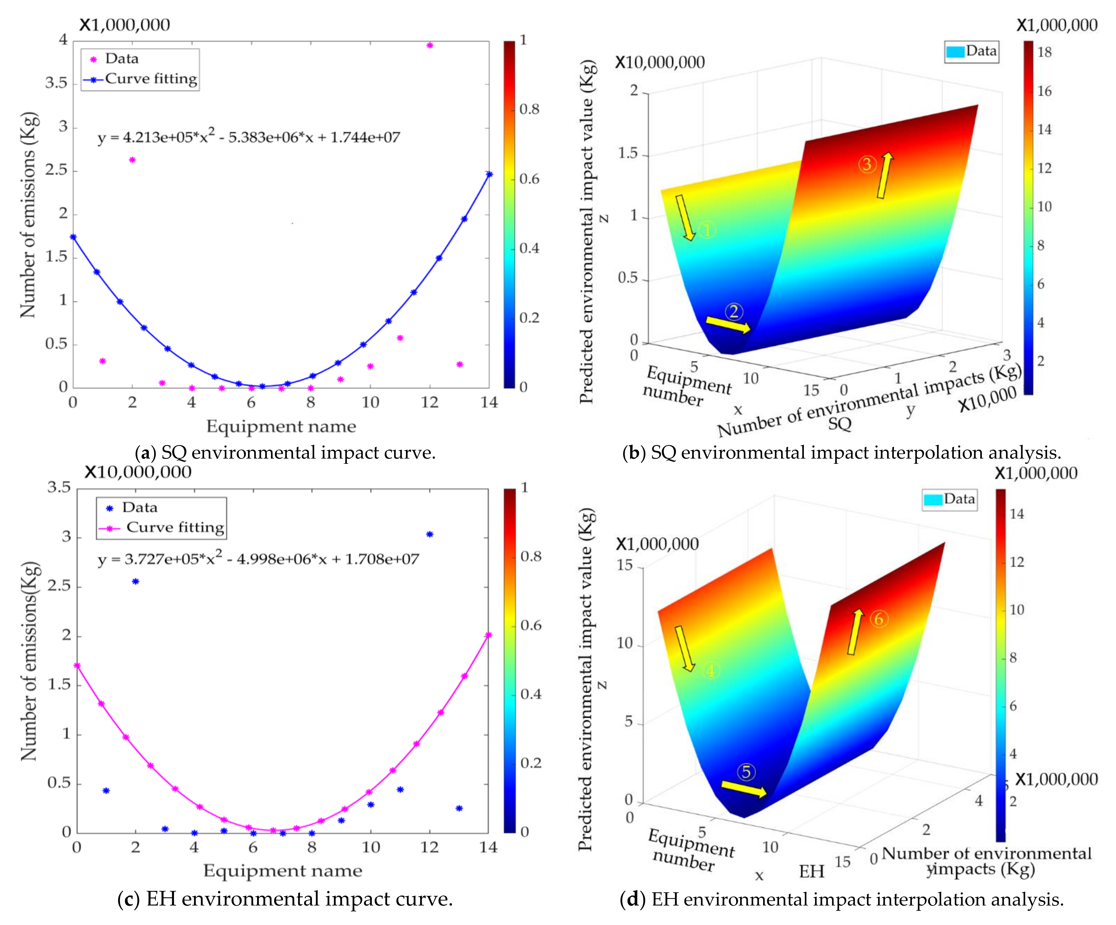
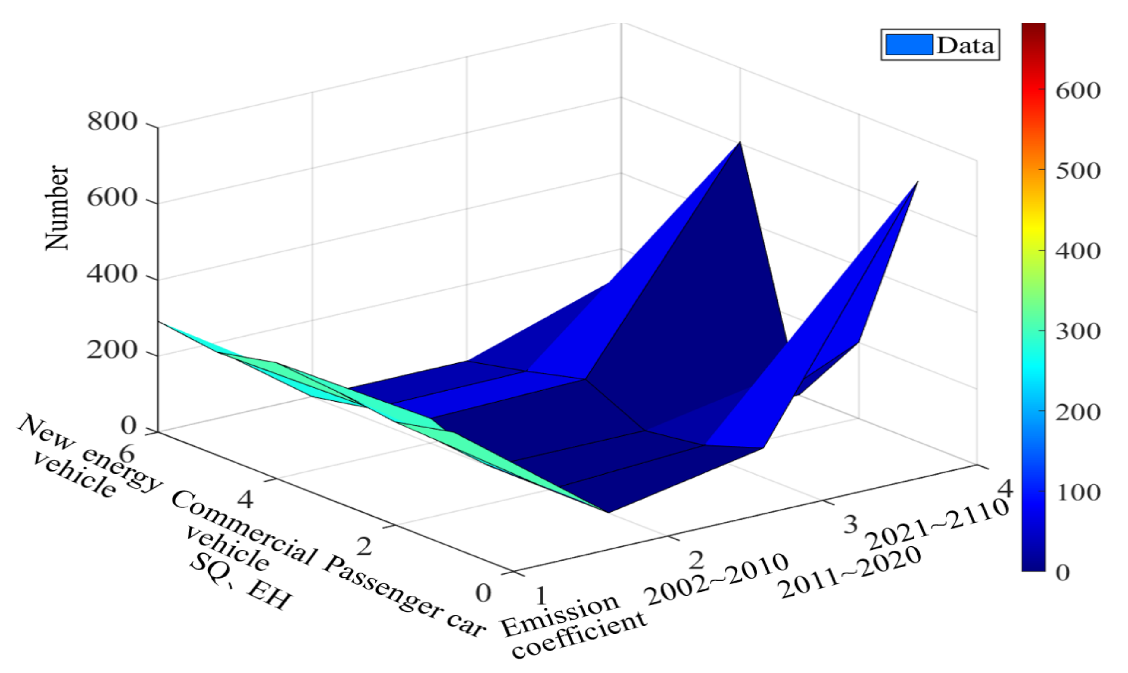
Figure 13 shows that in the maintenance and operation stage, the environmental impact value is larger for the replacement of the main beam (point 2) and the garbage pollution generated by the maintenance personnel (point 12). After the MATLAB scientific algorithm is fitted, the fitting equation is reached:
Fitting algorithm program:
>>%SQ: z=(4.213e + 05).*x^2−(5.383e + 06).*x + (1.744e + 07).
>>%EH: z=(3.727e + 05).*x.^2-(4.998e + 06).*x + (1.708e + 07).
>>clear all; % Curve equation fitting, The first set of calculation programming language;
>>x = [1 2 3 4 5 6 7 8 9 10 11 12 13];
>>y = [3175070.133 26344975.58 621212.387 14122.7683 41378.0309 17963.456 5.164350566 20075.328 1057111.776 2554272 5817825 39517468.41 2755301.595];
>>figure;
>>plot(x,y,‘bo’);
Interpolation analysis program:
>>Clear all;% The second set of calculation programming language;
>>x = 1:13;
>>y = 5:3175070;
>>[x,y] = meshgrid(x,y);
>>z = (4.213e+05).*x.^2−(5.383e + 06).*x + (1.744e+07);
>>figure;
>>surf(x,y,z);
>>colormap(‘jet’);
>>shading interp;
>>light(‘position’,[0.2 0.2 0.8]);
>>axis square;
>>xlabel(‘x’);
>>ylabel(‘y’);
>>zlabel(‘z’);
According to the fitted equation, the environmental impact change trend of SQ and EH during the 100-year maintenance period is calculated, which is divided into three stages. (1) The environmental impact value of materials, personnel, and equipment during the maintenance period is stable in a fixed area, indicated by (1)(4). (2) With the development of maintenance work, the originally installed equipment is in stable operation, without many equipment replacements (for example: main beams, main tower cables). Small materials are replaced (for example: guardrails, waterproof coating). The overall environmental impact contribution shows a downward trend, indicated by (2)(5). (3) With the replacement of large-scale equipment (such as main beams, main tower cables), the environmental impact value continues to increase, and the increasing trend is higher than the previous downward trend until the end of the 100-year operation period, as indicated by (3)(6). (4) Comparing SQ and EH, it can be found that the environmental impact change trend of EH during the maintenance period is higher than that of SQ.
5.2. Innovation
5.2.1. Modelling Analysis
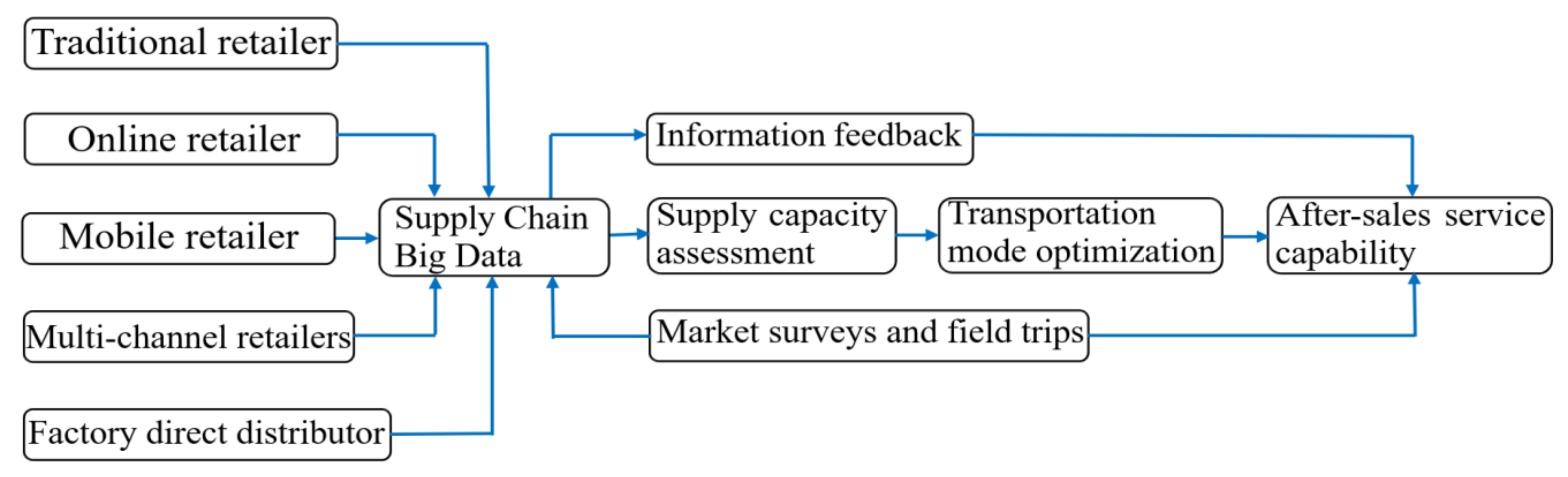
As the Internet and mobile communication technologies have advanced rapidly in the twenty-first century, reasonable use of big data to solve material procurement is of great significance. Cai et al. proposed an “Omni-Channel Management” framework and implemented omni-channel management [
74]. As shown in
Figure 5, the third level of the environmental emissions contribution of cable-stayed bridges can be divided into eight categories and 31 types. The impact factor is considered the variable node
, and the directed edges between nodes represent the interrelationships between nodes;
corresponds to the probability distribution
. The joint probability distribution for
nodes (
) can be expressed as:
The significance of each random variable’s impact on the environmental emission contribution can be expressed by the sensitivity.
and
represent the probability distribution of
and
;
represents the direct influence on the relationship between
and
:
Figure 14 introduces big data omni-channel assessment analysis to solve the serious traffic pollution problem of SQ and EH. The big data system analysis is used to select the best suppliers, assess the supply lines, and reduce the impact factors shown in Equation (11).
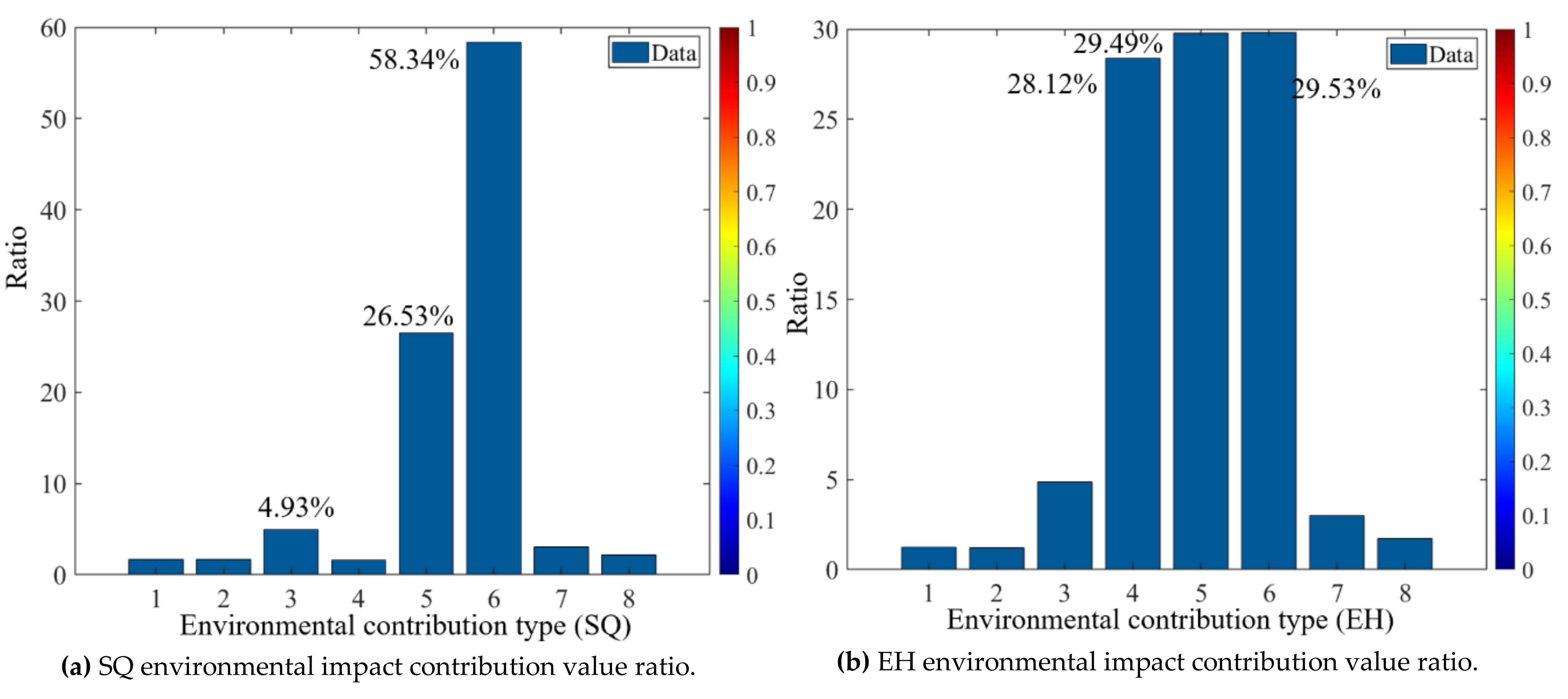
Figure 15 shows that SQ’s environmental impact factors are concentrated in the physicochemical energy of materials (43959.26 tonnes), garbage and sewage (43898.84 tonnes), and vehicles (41866.31 tonnes), accounting for 87.97% of the total. EH’s environmental impact factors are concentrated in physicochemical energy of materials (78944.70 tonnes) and garbage and sewage (35901.30 tonnes), accounting for 84.87% of the total.
The symbols 1-8 in
Figure 15 represent content: 1 = Construction equipment diesel contribution; 2 = Construction equipment electrical contribution; 3 = Human contribution and energy consumption; 4 = Transportation vehicle contribution; 5 = Contribution of garbage and sewage; 6 = Physical and chemical energy of various materials; 7 = Concrete carbonization; 8 = External environmental impact.
The following can be deduced from Equation (12):
= (1.24%, 1.20%, 4.86%, 28.39%, 29.77%, 29.81%, 2.99%, 1.73%)= (1.67%, 1.72%, 4.93%, 1.62%, 26.53%, 58.34%, 3.02%, 2.16%).
The following can be deduced from Equation (12):
According to the calculation result, the sensitivities of the eight categories of impact factors to environmental emission contributions can be ranked as follows:
= (23.324 > 14.082 > 6.302 > 2.781 > 2.145 > 1.367 > 1.357), and
= (8.736 > 7.799 > 6.217 > 5.689 > 5.073 > 2.650 > 1.269).
The conclusion of the sensitivity analysis is consistent with the research conclusion in
Section 5.1. Sensitivity analysis ranking shows that the smaller the sensitivity calculation value, the greater the number of pollution emission of the impact factor. This is consistent with the
and
ranking. The minimum value of
1.357 and the minimum value of
1.269 are the environmental pollution emissions of raw materials consumed in the maintenance and operation phases.
5.2.2. Measures
SQ and EH require the following measures. ① Designing and choosing energy-saving and environmentally friendly materials and reducing cement consumption. ② Disposing of waste materials in strict accordance with construction regulations [
68]. ③ Regular special garbage cleaning. ④ Strictly controlling the random discharge of garbage by construction workers.
The amounts of waste materials and wastewater generated by SQ are 527.51 tonnes and 749.27 m
3; the amounts of waste materials and wastewater generated by EH are 488.38 tonnes and 693.70 m
3. There is a need to install digital automatic control processing equipment for centralized recycling in the mixing plant [
75,
76,
77].
5.3. Transportation
The transportation emission analysis of the cable-stayed bridge is calculated according to the 100-year life span of the drawing design (2011–2110). Zhou et al. determined the equivalent environmental impact indicators for fuel-powered vehicles and BEVs [
78,
79,
80,
81,
82]. The research results show that the GWP emissions of new energy automobiles in the driving phase are between 197.17 and 284.72 g/km.
The upper limit of vehicle saturation in China is 807 vehicles/1000 people, and it will reach 390 million vehicles in 2030, which is 269 vehicles/1000 people [
83]. From 2030 to 2050, the growth rate will be 2.9%, reaching 455 vehicles/1000 people [
84]. Joyce Dargah et al., Tian Wu et al., and Zhou et al. established a theoretical model to measure vehicles.
5.3.1. Modelling in Operation and Maintenance Phase
The calculation model of the membership function can be built as follows, based on Equations (11) and (12)
where
is the contribution of transportation on SQ to environmental emissions in the maintenance and operation phase (kg);
,
, and
are the traffic volumes of different types of vehicles (per vehicle/year/km);
,
, and
are the environmental impact emissions indexes of different types of vehicles (g/km);
,
and
are the growth and reduction rates of different types of vehicles per year (%); and
is the fixed growth and reduction rate of different types of vehicles per year (%).
where
is the contribution of transportation on EH to environmental emissions in the maintenance and operation phase (kg).
Formula (13) shows the total sales volume and growth rate of the three types of automobiles in China from 2008 to 2019 [
85], based on the latest development plan for the new energy automobile industry issued by the State Council of China (2021–2035) to model (13) and (14) analyse the vehicle traffic on cable-stayed bridges.
5.3.2. Calculations in the Operation and Maintenance Phase
Table 8 shows the assessment vehicle data in the maintenance and operation phase, which are obtained using Equations (13) and (14) and [
78,
79,
80,
81,
82,
83]. The operating periods of SQ and EH are 2011–2110 and 2002–2102, respectively.
Figure 16 shows the assessment of transportation pollution by vehicle type. New-energy automobiles have disadvantages such as being limited to short distances, limited installation of supporting power supply facilities, and short battery life, so they are still in the stage of promotion in China and have a low market share. HEVs have overcome some of the defects of electric vehicles, but the conclusions obtained from the assessment analysis data are not obvious. At present, research and analysis concerning improving fuel quality standards and controlling exhaust emissions after combustion is an effective solution.
As shown in
Figure 17, the highest contribution to environmental emissions in the five phases of SQ is 1985.01 tonnes and is made in the disassembly and recycling stage. The reason for this is that SQ is far from the steel plant (330 km) and the waste power plant (846 km), resulting in high exhaust emissions. The reason for not choosing to dispose of wastes in the nearby waste treatment plant is to consider the reduction in secondary pollution, material regeneration, and secondary utilization. The highest exhaust emissions of EH total 1345.78 tonnes. After the modelling assessment and analysis of the transportation pollution of the two bridges, the pollution emissions decrease by 72.09 and 258.55 tonnes, respectively.
6. Conclusions
In the face of the serious pollution caused by the global construction industry, researchers from all over the world are working hard to find the research framework and methods to improve the LCA of bridges, to better reduce the environmental pollution and energy consumption of bridge engineering. At the same time, many uncertain factors have appeared in the research process.
In this work, the FMT and BN theoretical model is established to solve the interference problem of uncertainty factors in LCA. Combined with the five research theories of Monte Carlo simulation, geometric mean and geometric standard deviation set by OpenLCA software, the uncertainty in LCA research is well-handled. The model is checked and analyzed with case data and evaluated comprehensively. It is found that the research conclusions are surprisingly consistent, which verifies the accuracy and practicability of the theoretical model again.
The results show that the contribution of SQ and EH to the environment in the two stages of material manufacturing and maintenance and operation accounted for 26.64% and 26.38% and 55.57% and 53.57% of the total emissions, respectively. At the same time, the two stages of software analysis data were evaluated by BNFC. The results of SQ and EH maintenance stage model evaluation was 55.73% and 53.57%. The conclusion of theoretical model evaluation is almost consistent with that of software analysis.
Through the matching degree check and the comprehensive influence weight matrix verification of influence factors, it is found that the influence factors obtained by means of the three different research methods of the analytical hierarchy process based on BNFC, comprehensive evaluation of the BNFC and LCA software is very consistent with the factors assumed by fuzzy mathematics calculation, which proves the accuracy of 3.4.3 modelling.
Finally, the sensitivity analysis of the environmental severity in the maintenance and operation phase is carried out. It was found that the pollutants mainly concentrated in the physical and chemical energy of materials, garbage and sewage, and vehicles, accounting for 87.14% and 85.66% of the total emissions of SQ and EH. Through the optimization modelling again, the SQ emission is reduced by 72.09 tonnes, and the EH emission is reduced by 258.55 tonnes.
Theoretical research in basic science is the stepping-stone of applied science, and the solid FMT paves the way for solving the complex dynamic uncertainty. The results of this study prove that in the process of achieving the sustainable development goals of the construction industry, due to the complexity and uncertainty of the research objects and other factors, it is limited and unstable to rely solely on databases and software for analysis. It is aimed at new materials, new construction machinery, and new construction techniques. The key is to apply scientific methods to prove the accuracy and robustness of research conclusions through each layer of verification and proofreading steps in the theoretical framework model. The Bayesian network fuzzy number comprehensive evaluation model breaks through the constraints of software and database and achieves the purpose of research. Contributed to a more scientific realization of the sustainable development goals. The research results of this work can be used as ideas and methods to solve LCA research in other industries, and more research results are expected to verify them, in order to make better use of interdisciplinary theory to deal with the difficulties in the research. The limitation of this study is that there is no further research, analysis, and optimization of the other four stages in order to better reduce environmental pollution. In the future, we need to increase the research on the combination of fuzzy mathematics and topology optimization, to better contribute to reducing the environmental pollution of the construction industry.
Author Contributions
Investigation, Z.-W.Z. and J.A.; methodology, Z.-W.Z., J.A., and V.Y.; supervision, J.A, M.K. and V.Y.; validation, Z.-W.Z. and M.K.; writing—original draft, Z.-W.Z.; writing—review and editing, J.A, M.K. and V.Y. All authors have read and agreed to the published version of the manuscript.
Funding
This research was funded by the Spanish Ministry of Economy and Competitiveness, along with FEDER (Fondo Europeo de Desarrollo Regional), project grant number: BIA2017-85098-R.
Acknowledgments
The authors would like to thank the editor of the applied sciences and the anonymous reviewers for contributing to improve the earlier version of this manuscript.
Conflicts of Interest
The authors declare no potential conflict of interest with respect to the research, authorship, and/or publication of this article.
Nomenclature
| BN | Bayesian networks |
| LCA | Life cycle assessment |
| FMT | Fuzzy mathematics theory |
| BNFC | Bayesian network fuzzy number comprehensive evaluation |
| GWP | Global warming parameters |
| AP | Acidification parameters |
| FEP | Freshwater eutrophication parameters |
| PMFP | Particulate matter formation parameters |
| WP | Solid waste parameters |
| SQ | Su Qian bridge |
| EH | Gong He cable-stayed bridge |
| C | Concrete |
| Km | Kilometers |
| kwh | Kilowatt-hour |
References
- Yin, S.; Li, B.; Xing, Z. The governance mechanism of the building material industry (BMI) in transformation to green BMI: The perspective of green building. Sci. Total Environ. 2019, 677, 19–33. [Google Scholar] [CrossRef]
- Det Udomsap, A.; Hallinger, P. A bibliometric review of research on sustainable construction, 1994–2018. J. Clean. Prod. 2020, 254. [Google Scholar] [CrossRef]
- Akadiri, P.O.; Chinyio, E.A.; Olomolaiye, P.O. Design of a sustainable building: A conceptual framework for implementing sustainability in the building sector. Buildings 2012, 2, 126–152. [Google Scholar] [CrossRef]
- Brambilla, A.; Sangiorgio, A. Mould growth in energy efficient buildings: Causes, health implications and strategies to mitigate the risk. Renew. Sustain. Energy Rev. 2020, 132, 110093. [Google Scholar] [CrossRef]
- Banihashemi, S.A.; Khalilzadeh, M.; Shahraki, A.; Malkhalifeh, M.R.; Ahmadizadeh, S.S.R. Optimization of environmental impacts of construction projects: A time-cost-quality trade-off approach. Int. J. Environ. Sci. Technol. 2020, 1–16. [Google Scholar] [CrossRef]
- Bare, J.C.; Hofstetter, P.; Pennington, D.W.; Udo de Haes, H.A. Life cycle impact assessment workshop summary. Midpoints versus endpoints: The sacrifices and benefits. Int. J. Life Cycle Assess. 2000, 5, 319–326. [Google Scholar] [CrossRef]
- Ciroth, A.; Eisfeldt, F. PSILCA-A Product Social Impact Life Cycle Assessment Database; Database Version 1.0; Greendelta: Berlin, Germany, 2016; Available online: https://www.openlca.org/wp-content/uploads/2016/08/PSILCA_documentation_v1.1.pdf (accessed on 12 May 2021).
- Wei, J.; Cen, K. A preliminary calculation of cement carbon dioxide in China from 1949 to 2050. Mitig. Adapt. Strateg. Glob. Chang. 2019, 24, 1343–1362. [Google Scholar] [CrossRef]
- Arbault, D.; Rivière, M.; Rugani, B.; Benetto, E.; Tiruta-Barna, L. Integrated earth system dynamic modeling for life cycle impact assessment of ecosystem services. Sci. Total Environ. 2014, 472, 262–272. [Google Scholar] [CrossRef]
- Orcesi, A.; Cremona, C.; Ta, B. Optimization of design and life-cycle management for steel–concrete composite bridges. Struct. Eng. Int. 2018, 28, 185–195. [Google Scholar] [CrossRef]
- Zhou, Z.; Alcalá, J.; Yepes, V. Bridge carbon emissions and driving factors based on a life-cycle assessment case study: Cable-stayed bridge over Hun He river in Liaoning, China. Int. J. Environ. Res. Public Health 2020, 17, 5953. [Google Scholar] [CrossRef]
- Landi, D.; Marconi, M.; Bocci, E.; Germani, M. Comparative life cycle assessment of standard, cellulose-reinforced and end of life tires fiber-reinforced hot mix asphalt mixtures. J. Clean. Prod. 2020, 248, 119295. [Google Scholar] [CrossRef]
- Santos, R.; Costa, A.A.; Silvestre, J.D.; Vandenbergh, T.; Pyl, L. BIM-Based life cycle assessment and life cycle costing of an office building in Western Europe. Build. Environ. 2020, 169. [Google Scholar] [CrossRef]
- Cristiano, S.; Gonella, F. To build or not to build? Megaprojects, resources, and environment: An emergy synthesis for a systemic evaluation of a major highway expansion. J. Clean. Prod. 2019, 223, 772–789. [Google Scholar] [CrossRef]
- Giunta, M.; Bosco, D.L.; Leonardi, G.; Scopelliti, F. Estimation of gas and dust emissions in construction sites of a motorway project. Sustainability 2019, 11, 7218. [Google Scholar] [CrossRef]
- Crandall, C.S. Science as dissent: The practical value of basic and applied science. J. Soc. Issues 2019, 75, 630–641. [Google Scholar] [CrossRef]
- About Expertly curated abstract & citation database. Available online: https://www.elsevier.com/solutions/scopus (accessed on 22 April 2021).
- Thought Co. Official Listing of Countries by Region of the World. Available online: https://www.thoughtco.com/official-listing-of-countries-world-region-1435153 (accessed on 21 April 2021).
- Fritz Carrapatoso, A. Environmental aspects in free trade agreements in the Asia-Pacific region. Asia Eur. J. 2008, 6, 229–243. [Google Scholar] [CrossRef]
- Huang, L.; Krigsvoll, G.; Johansen, F.; Liu, Y.; Zhang, X. Carbon emission of global construction sector. Renew. Sustain. Energy Rev. 2018, 81, 1906–1916. [Google Scholar] [CrossRef]
- Chau, C.K.; Leung, T.M.; Ng, W.Y. A review on life cycle assessment, life cycle energy assessment and life cycle carbon emissions assessment on buildings. Appl. Energy 2015, 143, 395–413. [Google Scholar] [CrossRef]
- Onat, N.C.; Kucukvar, M.; Tatari, O. Scope-Based carbon footprint analysis of U.S. residential and commercial buildings: An input-output hybrid life cycle assessment approach. Build. Environ. 2014, 72, 53–62. [Google Scholar] [CrossRef]
- Kokoni, S.; Skea, J. Input-Output and life-cycle emissions accounting: Applications in the real world. Clim. Policy 2014, 14, 372–396. [Google Scholar] [CrossRef]
- Zhou, Z.; Alcalá, J.; Yepes, V. Environmental, economic and social impact assessment: Study of bridges in China’s five major economic regions. Int. J. Environ. Res. Public Health 2020, 18, 122. [Google Scholar] [CrossRef]
- Chuai, X.; Huang, X.; Lu, Q.; Zhang, M.; Zhao, R.; Lu, J. Spatiotemporal changes of built-up land expansion and carbon emissions caused by the Chinese construction industry. Environ. Sci. Technol. 2015, 49, 13021–13030. [Google Scholar] [CrossRef]
- Larsson Ivanov, O.; Honfi, D.; Santandrea, F.; Stripple, H. Consideration of uncertainties in LCA for infrastructure using probabilistic methods. Struct. Infrastruct. Eng. 2019, 711–724. [Google Scholar] [CrossRef]
- Wiedmann, T.; Lenzen, M. Environmental and social footprints of international trade. Nat. Geosci. 2018, 11, 314–321. [Google Scholar] [CrossRef]
- Hosny, A.; Nik-Bakht, M.; Moselhi, O. Workspace planning in construction: Non-Deterministic factors. Autom. Constr. 2020, 116, 103222. [Google Scholar] [CrossRef]
- Tae, S.; Baek, C.; Shin, S. Life cycle CO2 evaluation on reinforced concrete structures with high-strength concrete. Environ. Impact Assess. Rev. 2011, 31, 253–260. [Google Scholar] [CrossRef]
- Penadés-Plà, V.; García-Segura, T.; Martí, J.V.; Yepes, V. An optimization-LCA of a prestressed concrete precast bridge. Sustainability 2018, 10, 685. [Google Scholar] [CrossRef]
- Hosny, A.; Nik-Bakht, M.; Moselhi, O. Chaos and complexity in modeling and detection of spatial temporal clashes in construction processes. In Proceedings of the Construction Research Congress 2018, New Orleans, LA, USA, 2–4 April 2018; 2018; Volume 2018, pp. 639–648. [Google Scholar] [CrossRef]
- Bouhaya, L.; Le Roy, R.; Feraille-Fresnet, A. Simplified environmental study on innovative bridge structure. Environ. Sci. Technol. 2009, 43, 2066–2071. [Google Scholar] [CrossRef]
- Habert, G.; Arribe, D.; Dehove, T.; Espinasse, L.; Roy, R.L. Reducing environmental impact by increasing the strength of concrete: Quantification of the improvement to concrete bridges. J. Clean. Prod. 2012, 35, 250–262. [Google Scholar] [CrossRef]
- Navarro, I.J.; Penadés-Plà, V.; Martínez-Muñoz, D.; Rempling, R.; Yepes, V. Life cycle sustainability assessment for multi-criteria decision making in bridge design: A review. J. Civ. Eng. Manag. 2020, 26, 690–704. [Google Scholar] [CrossRef]
- Penadés-Plà, V.; Martí, J.V.; García-Segura, T.; Yepes, V. Life-Cycle assessment: A comparison between two optimal post-tensioned concrete box-girder road bridges. Sustainability 2017, 9, 1864. [Google Scholar] [CrossRef]
- Sánchez-Garrido, A.J.; Yepes, V. Multi-Criteria assessment of alternative sustainable structures for a self-promoted, single-family home. J. Clean. Prod. 2020, 258, 120556. [Google Scholar] [CrossRef]
- OpenLCA 1.10. Available online: https://www.openlca.org/openlca/ (accessed on 12 May 2021).
- Holický, M.; Marková, J.; Sýkora, M. Forensic assessment of a bridge downfall using Bayesian networks. Eng. Fail. Anal. 2013, 30, 1–9. [Google Scholar] [CrossRef]
- Carvalho, A.M. Scoring Functions for Learning Bayesian Networks. Inesc-id Tec. Rep. 2009, 12, 1–48. Available online: http://www.lx.it.pt/asmc/pub/talks/09-TA/ta_pres.pdf (accessed on 10 May 2021).
- Li, Y.F.; Liu, Y.; Huang, T.; Huang, H.Z.; Mi, J. Reliability assessment for systems suffering common cause failure based on Bayesian networks and proportional hazards model. Qual. Reliab. Eng. Int. 2020, 36, 2509–2520. [Google Scholar] [CrossRef]
- Khakzad, N.; Khan, F.; Amyotte, P. Risk-Based design of process systems using discrete-time Bayesian networks. Reliab. Eng. Syst. Saf. 2013, 109, 5–17. [Google Scholar] [CrossRef]
- Mentes, A.; Helvacioglu, I.H. An application of fuzzy fault tree analysis for spread mooring systems. Ocean Eng. 2011, 38, 285–294. [Google Scholar] [CrossRef]
- Shary, S.P. A new technique in systems analysis under interval uncertainty and ambiguity. Reliab. Comput. 2002, 8, 321–418. [Google Scholar] [CrossRef]
- Inuiguchi, M.; Ramík, J.; Tanino, T. Oblique fuzzy vectors and their use in possibilistic linear programming. Fuzzy Sets Syst. 2003, 135, 123–150. [Google Scholar] [CrossRef]
- Zio, E. Reliability engineering: Old problems and new challenges. Reliab. Eng. Syst. Saf. 2009, 94, 125–141. [Google Scholar] [CrossRef]
- Straub, D.; Papaioannou, I. Bayesian updating with structural reliability methods. J. Eng. Mech. 2015, 141, 04014134. [Google Scholar] [CrossRef]
- Luque, J.; Straub, D. Reliability analysis and updating of deteriorating systems with dynamic Bayesian networks. Struct. Saf. 2016, 62, 34–46. [Google Scholar] [CrossRef]
- Dubois, D.; Esteva, F.; Godo, L.; Prade, H. Fuzzy-Set based logics-an history-oriented presentation of their main developments. Many Valued Nonmonotonic Turn Log. 2007, 8, 1–125. [Google Scholar] [CrossRef]
- Zhu, L. Research and application of AHP-fuzzy comprehensive evaluation model. Evol. Intell. 2020, 1, 3. [Google Scholar] [CrossRef]
- Bao, Z.; Mehran, K.; Lam, H.K.; Li, X. Membership-Dependent stability analysis of discrete-time positive polynomial fuzzymodel-based control systems with time delay. IET Control Theory Appl. 2020, 14, 1135–1146. [Google Scholar] [CrossRef]
- Ecoinvent Database. Available online: https://www.ecoinvent.org/database/ecoinvent (accessed on 10 May 2021).
- Bedec Datebase. Available online: https://en.itec.cat/database/ (accessed on 20 May 2021).
- Hoogmartens, R.; Van Passel, S.; Van Acker, K.; Dubois, M. Bridging the gap between LCA, LCC and CBA as sustainability assessment tools. Environ. Impact Assess. Rev. 2014, 48, 27–33. [Google Scholar] [CrossRef]
- Yang, X.; Hu, M.; Wu, J.; Zhao, B. Building-Information-Modeling enabled life cycle assessment, a case study on carbon footprint accounting for a residential building in China. J. Clean. Prod. 2018, 183, 729–743. [Google Scholar] [CrossRef]
- Rahimi, M.; Weidner, M. Decision analysis utilizing data from multiple life-cycle impact assessment methods: Part II: Model Development. J. Ind. Ecol. 2008, 8, 119–141. [Google Scholar] [CrossRef]
- Wang, C.Q.; Li, Z.L.; Yan, Z.T.; Xiao, Z.Z. Experimental investigation on wind-resistant behavior of Chaotianmen Yangtze River Bridge. Exp. Tech. 2012, 36, 26–38. [Google Scholar] [CrossRef]
- Zhou, Z.; Meng, S.P.; Liu, Z. Practical computing method of longitudinal anti-crack analysis for anchor end of wide hollow slab girders. Gongcheng Lixue Eng. Mech. 2008, 25, 177–183. [Google Scholar]
- Code for Investigation of Geotechnical Engineering GB 50021-2001. Ministry of Housing and Urban-Rural Development of the People’s Republic of China, Beijing, China. 2002. Available online: http://www.jianbiaoku.com/webarbs/book/246/54830.shtml (accessed on 20 April 2021). (In Chinese).
- Bao, H.; Yu, M.; Xu, L.; Saafi, M.; Ye, J. Experimental study and multi-physics modelling of concrete under supercritical carbonation. Constr. Build. Mater. 2019, 227. [Google Scholar] [CrossRef]
- Sun, B.; Xiao, R.-C.; Ruan, W.-D.; Wang, P.-B. Corrosion-Induced cracking fragility of RC bridge with improved concrete carbonation and steel reinforcement corrosion models. Eng. Struct. 2020, 208. [Google Scholar] [CrossRef]
- Vora, P.R.; Dave, U.V. Parametric studies on compressive strength of geopolymer concrete. In Procedia Engineering; Elsevier Ltd.: Amsterdam, The Netherlands, 2013; Volume 51, pp. 210–219. [Google Scholar] [CrossRef]
- Ta, V.L.; Bonnet, S.; Senga Kiesse, T.; Ventura, A. A new meta-model to calculate carbonation front depth within concrete structures. Constr. Build. Mater. 2016, 129, 172–181. [Google Scholar] [CrossRef]
- Standard for durability assessment of existing concrete structures. 2019. Available online: http://www.jianbiaoku.com/webarbs/book/138893/4047181.shtml (accessed on 20 April 2021). (In Chinese).
- Li, F.; Luo, X.; Liu, Z. Corrosion of anchorage head system of post-tensioned prestressed concrete structures under chloride environment. Struct. Concr. 2017, 18, 902–913. [Google Scholar] [CrossRef]
- Tam, V.W.Y. Economic comparison of concrete recycling: A case study approach. Resour. Conserv. Recycl. 2008, 52, 821–828. [Google Scholar] [CrossRef]
- Engelsen, C.J.; Mehus, J.; Pade, C.; Sæther, D.H. Carbon dioxide uptake in demolished and crushed concrete - CO2 Uptake During the Concrete Life Cycle, BYGGFORSK Norwegian Building Research Institute Project 03018 report 395−2005. 2005. Available online: https://www.sintef.no/globalassets/upload/byggforsk/publikasjoner/ (accessed on 14 May 2021).
- Yuan, H. Critical management measures contributing to construction waste management: Evidence from construction projects in China. Proj. Manag. J. 2013, 44, 101–112. [Google Scholar] [CrossRef]
- Nan, C.; Jie, Z. Concrete construction waste pollution and relevant prefabricated recycling measures. Nat. Environ. Pollut. Technol. Int. Q. Sci. J. 2020, 19, 367–372. [Google Scholar]
- Milani, C.J.; Yepes, V.; Kripka, M. Proposal of sustainability indicators for the design of small-span bridges. Int. J. Environ. Res. Public Health 2020, 17, 4488. [Google Scholar] [CrossRef]
- IPCC, 2014: Climate Change 2014: Synthesis Report. In Contribution of Working Groups I, II and III to the Fifth Assessment Report of the Intergovernmental Panel on Climate Change; Core Writing Team, Pachauri, R.K., Meyer, L.A., Eds.; IPCC: Geneva, Switzerland, 2015; p. 151. ISBN 978-92-9169-143-2. Available online: https://www.ipcc.ch/report/ar5/syr/ (accessed on 10 May 2021).
- Martínez-Munõz, D.; Martí, J.V.; Yepes, V. Steel-Concrete composite bridges: Design, life cycle assessment, maintenance, and decision-making. Adv. Civ. Eng. 2020, 8823370. [Google Scholar] [CrossRef]
- Zhao, S.; Song, Q.; Duan, H.; Wen, Z.; Wang, C. Uncovering the lifecycle GHG emissions and its reduction opportunities from the urban buildings: A case study of Macau. Resour. Conserv. Recycl. 2019, 147, 214–226. [Google Scholar] [CrossRef]
- Chung, S.S.; Wing-Hung Lo, C. Evaluating sustainability in waste management: The case of construction and demolition, chemical and clinical wastes in Hong Kong. Resour. Conserv. Recycl. 2003, 37, 119–145. [Google Scholar] [CrossRef]
- Cai, Y.J.; Lo, C.K.Y. Omni-Channel management in the new retailing era: A systematic review and future research agenda. Int. J. Prod. Econ. 2020, 229. [Google Scholar] [CrossRef]
- De Haas, K.; Wilsdorf, D.; Schlösser, J. Process instrumentation, control equipment, and process analysis measurement technology. In Multiproduct Plants; Wiley-VCH Verlag GmbH & Co. KGaA: Weinheim, Germany, 2005; pp. 131–158. [Google Scholar] [CrossRef]
- Yepes, V.; Dasí-Gil, M.; Martínez-Muñoz, D.; López-Desfilis, V.J.; Martí, J.V. Heuristic techniques for the design of steel-concrete composite pedestrian bridges. Appl. Sci. 2019, 9, 3253. [Google Scholar] [CrossRef]
- Siddiqui, S.A.; Ahmad, A. Implementation of thin-walled approximation to evaluate properties of complex steel sections using C++. SN Comput. Sci. 2020, 1. [Google Scholar] [CrossRef]
- State Council of China. New Energy Automobile Industry Development Plan (2012–2020). 2012. Available online: http://www.gov.cn/zhengce/ (accessed on 20 April 2021).
- Sierra, L.A.; Pellicer, E.; Yepes, V. Method for estimating the social sustainability of infrastructure projects. Environ. Impact Assess. Rev. 2017, 65, 41–53. [Google Scholar] [CrossRef]
- Qiao, Q.; Zhao, F.; Liu, Z.; Hao, H. Electric vehicle recycling in China: Economic and environmental benefits. Resour. Conserv. Recycl. 2019, 140, 45–53. [Google Scholar] [CrossRef]
- Figueiredo, K.; Pierott, R.; Hammad, A.W.A.; Haddad, A. Sustainable material choice for construction projects: A life cycle sustainability assessment framework based on BIM and Fuzzy-AHP. Build. Environ. 2021, 196, 107805. [Google Scholar] [CrossRef]
- Huang, M.; Dong, Q.; Ni, F.; Wang, L. LCA and LCCA based multi-objective optimization of pavement maintenance. J. Clean. Prod. 2021, 283. [Google Scholar] [CrossRef]
- Dargay, J.; Gately, D.; Sommer, M. Vehicle ownership and income growth, worldwide: 1960–2030. Energy J. 2007, 28, 143–170. [Google Scholar] [CrossRef]
- Wu, T.; Zhang, M.; Ou, X. Analysis of future vehicle energy demand in China based on a gompertz function method and computable general equilibrium model. Energies 2014, 7, 7454–7482. [Google Scholar] [CrossRef]
- Schwabe, J. From “obligated embeddedness” to “obligated Chineseness”? Bargaining processes and evolution of international automotive firms in China’s New Energy Vehicle sector. Growth Chang. 2020, 51, 1102–1123. [Google Scholar] [CrossRef]
Figure 1.
Cluster analysis of published articles.
Figure 1.
Cluster analysis of published articles.
Figure 2.
Schematic diagram of BN principle.
Figure 2.
Schematic diagram of BN principle.
Figure 3.
The basic methods and steps of FMT comprehensive evaluation.
Figure 3.
The basic methods and steps of FMT comprehensive evaluation.
Figure 4.
Schematic diagram illustrating the single factor influence weight matrix.
Figure 4.
Schematic diagram illustrating the single factor influence weight matrix.
Figure 5.
Schematic diagram of tree-shaped BN of environmental impact contribution of cable-stayed bridge.
Figure 5.
Schematic diagram of tree-shaped BN of environmental impact contribution of cable-stayed bridge.
Figure 6.
Schematic diagram of two bridges.
Figure 6.
Schematic diagram of two bridges.
Figure 7.
Comparison diagram of research and analysis conclusions of SQ’s contribution to the environment.
Figure 7.
Comparison diagram of research and analysis conclusions of SQ’s contribution to the environment.
Figure 8.
Comparison diagram of research and analysis conclusions of EH environmental impact contribution.
Figure 8.
Comparison diagram of research and analysis conclusions of EH environmental impact contribution.
Figure 9.
Comparison of the conclusions of using two methods to study the environmental impact contribution of SQ and EH.
Figure 9.
Comparison of the conclusions of using two methods to study the environmental impact contribution of SQ and EH.
Figure 10.
The matching degree of the contribution of SQ and EH to the environmental impact is fit to the numerical curve.
Figure 10.
The matching degree of the contribution of SQ and EH to the environmental impact is fit to the numerical curve.
Figure 11.
The influencing factors obtained by the three evaluation methods are compared and fitted with the analysis of mean difference.
Figure 11.
The influencing factors obtained by the three evaluation methods are compared and fitted with the analysis of mean difference.
Figure 12.
Chart of impact factor deviation analysis for SQ and EH.
Figure 12.
Chart of impact factor deviation analysis for SQ and EH.
Figure 13.
SQ and EH maintenance and operation stage environmental impact fitting and future change trend interpolation analysis.
Figure 13.
SQ and EH maintenance and operation stage environmental impact fitting and future change trend interpolation analysis.
Figure 14.
Schematic diagram of big data omnichannel assessment framework.
Figure 14.
Schematic diagram of big data omnichannel assessment framework.
Figure 15.
A schematic diagram of the numerical comparison of the environmental impact contribution types of SQ and EH.
Figure 15.
A schematic diagram of the numerical comparison of the environmental impact contribution types of SQ and EH.
Figure 16.
A Summary table of vehicle assessment data during operation and maintenance for SQ and EH.
Figure 16.
A Summary table of vehicle assessment data during operation and maintenance for SQ and EH.
Figure 17.
Five-stage contribution of transportation vehicles and operation and maintenance vehicle assessment chart for SQ and EH.
Figure 17.
Five-stage contribution of transportation vehicles and operation and maintenance vehicle assessment chart for SQ and EH.
Table 1.
Data summary table for the survey and design stage.
Table 1.
Data summary table for the survey and design stage.
| Bridge Name | Design Institute and Project Site | Design Time | Survey and Design Time (Days) | Project Staff (Person) | Number of Drilling Holes | Drilling Depth | Drilling Working Hours |
|---|
| (km) | (Days) | Survey | Design | Survey | Design | (Piece) | (m) | (Hours) |
|---|
| SQ | 6 | 360 | 120 | 240 | 12 | 16 | 26 | 1456 | 11 |
| EH | 389 | 821 | 173 | 648 | 14 | 20 | 34 | 2210 | 16 |
Table 2.
Data summary table for construction.
Table 2.
Data summary table for construction.
| Bridge Name | Duration of the Hanging Basket (Days) | Total Construction Period (Days) | Main Tower Lifting Equipment | Working Power
(kwh) | Equipment Weight
(Tonnes) | Managed Personnel
(Persons) | Construction Worker
(Persons) |
|---|
| SQ | 255 | 729 | Tower crane | 90 | 78.54 | 24 | 260~320 |
| EH | 495 | 601 | Tower crane | 82.4 | 72.15 | 28 | 280~340 |
Table 3.
Maintenance and repair data.
Table 3.
Maintenance and repair data.
| SQ, EH Maintenance and Repair Cycle |
|---|
| Material | Damage Mechanism | Cycle |
|---|
| Steel | Aging; carbonization; rust; chloride salt corrosion; freeze–thaw environment; sulfate corrosion; alkali aggregation reaction | Maintenance/1 Year |
| Inspection and repair/2 Years |
| Maintenance and repair/70 Years |
| Expansion joint; Waterproof level; Bridge deck pavement | Wear; aging; chloride salt corrosion; freeze–thaw environment; sulfate corrosion; destruction | Maintenance/1 Year |
| Inspection and repair/2 Years |
| Replacement/10Years |
| Main beam; Anti-collision guardrail; Bridge deck drainage; Lighting | Shock; vibration; overload; uneven settlement; chloride salt corrosion; freeze–thaw environment; sulfate corrosion; alkaline material reaction | Maintenance/1 Year |
| Inspection and repair/5 Years |
| Replacement/50Years |
| Paint for caps; Piers and beams | Chemical attack; abrasion; erosion; aging; chloride salt attack; freeze–thaw environment; sulfate attack | Maintenance/1 Year |
| Replacement/5Years |
| Abutment | Chemical attack; wear; impact; aging | Maintenance/1 Year |
| Inspection and repair/5 Years |
| Replacement/25Years |
| Main Galasso | Chemical corrosion; vehicle overload and insufficient maintenance | Maintenance/1 Year |
| Inspection and repair/5 Years |
| Replacement/30Years |
Table 4.
Summary table of five-stage modelling formulas [
11].
Table 4.
Summary table of five-stage modelling formulas [
11].
| Stage | Modelling Formula | Explanation |
|---|
| SD | +++++ | (kg); is EEC (kg); is the worker EC (kg) |
| MM | ++++ | is PGGDSEC (kg); is the material EC (kg) |
| CI | ++ | is the EC of power and fuel consumption during construction (kg) |
| MO | =++(8) + (9) + (10) + | is TVEC (kg); is the EC number (kg) |
| DR | +++ | is OFEC (kg) |
Table 5.
Summary table of bridge environmental impact contributions (
Table 4 formula calculation).
Table 5.
Summary table of bridge environmental impact contributions (
Table 4 formula calculation).
| Environmental Contribution Stage | Bridge Name | GWP (kg) | AP (kg) | FEP (kg) | PMFP (kg) | WP (kg) | Transportation Contribution (kg) | The Proportion |
|---|
| Survey and design | SQ | 322,603.10 | 0.29 | 1444.66 | 14.12 | 5609.22 | 4525.62 | 1.37% |
| EH | 6,075,65.23 | 0.52 | 2781.15 | 27.12 | 10,798.15 | 12,504.05 | 2.01% |
| Material manufacturing | SQ | 35,783,970.10 | 338,386.32 | 218,677.39 | 1,027,034.48 | 1,911,752.52 | 551,965.85 | 1.41% |
| EH | 32,607,070.35 | 297,990.71 | 193,603.27 | 915,282.34 | 1,679,151.52 | 554,608.67 | 1.55% |
| Construction and installation | SQ | 21,604,311.50 | 334.85 | 22,516.66 | 1212.05 | 86,335.68 | 98,670.19 | 0.45% |
| EH | 23,954,772.44 | 337.00 | 29,475.12 | 1389.47 | 113,471.60 | 89,074.70 | 0.37% |
| Maintenance and operation | SQ | 79,173,042.18 | 155,891.23 | 514,843.27 | 702,336.77 | 1,390,668.18 | 1,057,111.78 | 1.29% |
| EH | 69,602,711.16 | 238,252.02 | 466,229.79 | 850,705.27 | 1,325,559.61 | 1,345,777.99 | 1.86% |
| Disassembly and recycling | SQ | 4,184,764.66 | 43.94 | 234.27 | 31.98 | 891.24 | 1,985,014.96 | 47.42% |
| EH | 2,412,687.90 | 12.23 | 316.02 | 11.24 | 1222.36 | 194,206.26 | 8.04% |
Table 6.
Summary table of membership data of two cable-stayed bridge classification systems.
Table 6.
Summary table of membership data of two cable-stayed bridge classification systems.
| Types of EC | Bridge Name | Analysis Value (kg) | V1 | V2 | V3 | V4 | V5 |
|---|
| GWP | SQ | 141,068,691.53 | 0.23% | 25.37% | 15.31% | 56.12% | 2.97% |
| EH | 129,184,807.08 | 0.47% | 25.24% | 18.54% | 53.88% | 1.87% |
| AP | SQ | 494,656.64 | 0.00% | 68.41% | 0.07% | 31.52% | 0.01% |
| EH | 536,917.19 | 0.00% | 55.50% | 0.06% | 44.43% | 0.00% |
| FEP | SQ | 757,716.26 | 0.19% | 28.86% | 2.97% | 67.95% | 0.03% |
| EH | 693,040.75 | 0.40% | 27.94% | 4.25% | 67.36% | 0.05% |
| PMFP | SQ | 1,730,629.40 | 0.00% | 59.34% | 0.07% | 40.58% | 0.00% |
| EH | 1,768,574.83 | 0.00% | 51.75% | 0.08% | 48.17% | 0.00% |
| WP | SQ | 3,395,256.84 | 0.17% | 51.75% | 0.08% | 48.17% | 0.00% |
| EH | 3,132,009.78 | 0.34% | 53.61% | 3.62% | 42.38% | 0.04% |
Table 7.
Summary table of assessment factor weight data for two cable-stayed bridges.
Table 7.
Summary table of assessment factor weight data for two cable-stayed bridges.
| Impact Factor | Bridge Name | GWP | AP | FEP | PMFP | WP |
|---|
| SQ | 0.96% | 0.00% | 0.01% | 0.01% | 0.02% |
| EH | 0.95% | 0.00% | 0.01% | 0.01% | 0.02% |
| SQ | 20.00% | 20.00% | 20.00% | 20.00% | 20.00% |
| EH | 20.00% | 20.00% | 20.00% | 20.00% | 20.00% |
| SQ | 0.0478% | 0.0002% | 0.0003% | 0.0006% | 0.0012% |
| EH | 0.0477% | 0.0002% | 0.0003% | 0.0007% | 0.0012% |
| SQ | 0.9567% | 0.0034% | 0.0051% | 0.0117% | 0.0230% |
| EH | 0.9547% | 0.0040% | 0.0051% | 0.0131% | 0.0231% |
Table 8.
Summary table of assessment vehicle data analysis for SQ and EH.
Table 8.
Summary table of assessment vehicle data analysis for SQ and EH.
| Bridge Name | Car Type | Emission Coefficient (g/km) | 2002~2011 Year | 2011~2020 Year | 2021~2110 Year |
|---|
| Number of Passing Vehicles (Units) |
|---|
| SQ | Passenger car | 305.4g/km | 0.00 | 250,608.00 | 2,243,160.00 |
| Commercial vehicle | 271.8g/km | 0.00 | 82,896.00 | 735,480.00 |
| New energy vehicle | 292.5g/km | 0.00 | 387.00 | 3010.00 |
| EH | Passenger car | 305.4g/km | 212,700.00 | 243,156.00 | 1,982,869.33 |
| Commercial vehicle | 271.8g/km | 110,400.00 | 125,592.00 | 1,023,578.67 |
| New energy vehicle | 292.5g/km | 0.00 | 36.00 | 255.11 |
| Publisher’s Note: MDPI stays neutral with regard to jurisdictional claims in published maps and institutional affiliations. |
© 2021 by the authors. Licensee MDPI, Basel, Switzerland. This article is an open access article distributed under the terms and conditions of the Creative Commons Attribution (CC BY) license (https://creativecommons.org/licenses/by/4.0/).


