1. Introduction
To acquire an accurate signal from its sampling signal, the sampling rate should be at least the Nyquist rate, i.e., twice of the signal’s highest frequency component. However, high sampling rate results in expensive hardware resources. With the bandwidth of signals increasing rapidly, it leads to tremendous pressure on the hardware system. Moreover, traditional sampling methods may easily result in the huge waste of computation and storage resources, even leading to large recovery errors.
Compressed sensing (CS) theory proposed by D. Donoho, E. Candes and T. Tao successfully addressed these issues. According to the theory, if a signal is sparse in a certain domain, a measurement matrix unrelated to the sparse basis can be employed for low-dimensional projection, and a high-precision reconstruction can be accomplished through convex optimization algorithms or matching pursuit methods [
1]. B. Adcock provided mathematical explanations for CS by constructing frameworks and generalization concepts [
2].
Compared with traditional signal acquisition and processing, CS samples signals at a much lower sampling rate efficiently, compresses the number of measurements which require to be transmitted or processed, and acquires high-resolution signals with the characteristics of signals sparsity [
3,
4]. Because of the superior performance in signal sampling and compression, CS has been widely employed in the fields of wireless communications [
5], image and data processing [
6,
7], data compression [
8], signal denoising [
9,
10], especially in the real-time monitoring and analysis of vehicle signal quality [
11,
12,
13].
Vehicle is an organic coupled composition which consists of different sophisticated subsystems. With the explosive growth of ubiquitous vehicles, large numbers of sophisticated and complex devices are continually integrated to vehicle electronics. This leads to the essential need that we should acquire a sufficiently high-quality status signal for vehicle health monitoring. To provide reliable guarantees for the healthy operation of a vehicle, real-time monitoring of status signals in the vehicle system is a promising solution. Due to the large variety of vehicle signals and requirement for long-term supervising, real-time monitoring generates huge amounts of data, which presents extremely high requirements for signal sampling and storage. The conventional monitoring scheme for vehicle is depicted in
Figure 1a. The original signals are sampled and stored at a high sampling rate, which generates massive signals and imposes a heavy burden on storage and transmission [
14]. In order to transmit such sampling signals to the data processing center, it requires expensive hardware resources and causes large time delay. CS theory, which performs signals sampling and compression simultaneously, can be well employed in quality analysis for vehicle system. Real-time health monitoring for vehicle using CS is demonstrated in
Figure 1b. By contrast, only small numbers of measurement signals need to be transmitted after the original signals are sensed and compressed. In general, the data center has powerful computing resources to reconstruct the original signal. The transmission of these measurement signals demands limited resources and is extremely quick, which can be beneficial for the subsequent analysis and diagnosis.
Reconstruction refers to the procedure of recovering the original signal from the low-dimensional measurement signal, and it is the critical part of CS. Reconstruction algorithms can be mainly divided into two directions, i.e., convex optimization algorithms and iterative greedy methods [
8]. Convex optimization algorithms, such as basis pursuit (BP), require high computational complexity, which means they are not applicable in practice. By contrast, iterative greedy methods, proposed for handling the
l0-norm minimization, show advantages with low computational complexity and superior visual interpretation, and have aroused much attention.
The conventional greedy methods require prior knowledge of the sparse signal and perform expensively [
14,
15,
16,
17,
18]. Sparsity adaptive matching pursuit (SAMP) does not rely on sparsity level [
19]. With the potential performance advancement of SAMP, an increasing number of researchers have explored adaptive matching pursuit algorithms [
20,
21,
22,
23,
24,
25]. However, these algorithms do not employ the preselection step, i.e., making no initial estimation for sparsity level during the initial phase. This leads to poor reconstruction performance. In addition, they may hardly adopt appropriate variable step-size and do not further filter results for higher accuracy. Although these algorithms can perform reconstruction with rare prior information of signal sparsity level, the accuracy and efficiency of reconstruction still need to be greatly improved, especially for vehicle health monitoring.
To overcome problems mentioned above, we propose a novel greedy algorithm called filtering-based regularized sparsity variable step-size matching pursuit (FRSVssMP), which is capable of signal reconstruction with requiring no prior knowledge on the sparsity level. With the proposed initial estimation approach for signal sparsity level, this algorithm integrates strategies of regularization and variable step-size adaptive, and further filters reconstruction results. To verify the efficiency of FRSVssMP in reconstruction, we conducted lots of experiments on the typical vehicle signals. The results demonstrate that the proposed FRSVssMP surpasses other greedy algorithms both in terms of accuracy and efficiency. The proliferation of smart transportation has significantly promoted explosive growth of vehicles. Due to the sophisticated and complex electronics, vehicles are inevitably susceptible to various faults. Especially, with the rapid development of intelligent sensors, large numbers of heterogeneous vehicle status data impose heavy pressures in health monitoring. In order to ensure the reliable operation of vehicles and identify potential faults efficiently, FRSVssMP can serve as a promising paradigm to facilitate the transmission and analysis of those data. The contributions of this paper are three-fold, as follows:
Firstly, we put forward an initial estimation approach for signal sparsity level to exploit structure of the sparse signal.
Secondly, we propose a novel iterative greedy algorithm relying on no prior information of signal sparsity level. The algorithm integrates strategies of regularization and variable adaptive step size. Further, the original signal can be reconstructed precisely with the filtering mechanism.
Thirdly, extensive numerical simulations are conducted to verify the performance of the proposed algorithm for real-time health monitoring. Experimental results demonstrate that FRSVssMP significantly outperforms the state-of-the-art greedy algorithms.
The remainder of this paper is organized as follows. The basic model of CS and representative greedy algorithms are illustrated in
Section 2.
Section 3 gives the detailed description of sparsity level estimation approach and the proposed reconstruction algorithm. Simulation results and discussions are presented with typical disturbance signals, including synthetic sparse signals and real sparse signals in monitoring for the vehicle power system in
Section 4, followed by the conclusion in
Section 5.
3. The Proposed Algorithm and Its Applications
In this section, we propose a novel greedy algorithm FRSVssMP, which can be capable of signal reconstruction without requiring prior knowledge on the signal sparsity. With the proposed initial estimation approach for signal sparsity level, this algorithm integrates strategies of regularization and variable step-size adaptive, and further filters reconstruction results. Since the initial step size, which affects recovery performance obviously, is closely related to signal sparsity, this section presents a new approach to estimate signal sparsity level initially. In the following parts, regularization [
16], variable step-size adaptive [
19,
20,
21], and filtering mechanism are introduced, followed by the description of steps in details.
Regularization: As illustrated in [
16], regularization means to select a set of atoms with maximum energy, of which the maximum absolute value obtained by multiplying column vectors of the sensing matrix and residual is less than twice of the minimum one.
Sparsity variable step-size adaptive: As illustrated in [
20], adaptive variable step-size is a powerful step to improve reconstruction accuracy and efficiency. In this paper, we elaborate a new variable step-size pattern with comparison of thresholds and relative error. The idea of adaptive step-size utilized in [
20,
21] only adopts one stage of variant step sizes. By contrast, in our algorithm, two stages of variant step sizes are leveraged to further approximate the true signal sparsity level. In the initial phase, a large step size is adopted for rapid approximation. Until the precision reaches a certain high value, a small step size is utilized for accurate approximation. Adaptation is reflected in the setting of a small step size, which can be self-tuning according to characteristics of signals.
Filtering mechanism: Further, the filtering mechanism is proposed to exclude the incorrect supports. After aforementioned steps, the sparse signal can be obtained based upon the confirmed support set by least square method. However, without any prior information of signal sparsity, we are still unable to identify whether the estimated sparsity level is correct enough since the algorithm cannot traverse each possible sparsity. After numerous experiments, we find that for many applications, there is a high probability that the estimated sparsity level is larger than the actual level. In this case, we consider to further filter results for the sake of higher recovery accuracy. Filtering mechanism removes an atom that exerts minimal influence on reconstruction performance in each iteration until the residual cannot be further diminished.
Since the initial sparsity level estimation exerts an important influence on the subsequent steps, an initial estimation approach for the sparsity level is introduced. Then, the complete steps of the proposed algorithm are illustrated in detail.
3.1. An Initial Estimation Approach for the Signal Sparsity Level
Consider a sparse signal of sparsity level K (K << N). The true support set of sparse signals is denoted by , then we have . is the measurement vector and A is the sensing matrix. Support that , the i-th element of is the inner product of (the i-th column of A) and the measurement vector y, i.e., . The indices of the k0 (1 ≤ k0 ≤ N) largest absolute values in are merged into the identified support set , i.e., . denotes the restricted isometry constant. Now we can have the proposition 1.
Proposition 1:
Consider that A satisfies the RIP with parameters.
For, Proof of Proposition 1:
Put indices of the
K (1 ≤
K ≤
N) largest absolute values in
to be
. If
k0 ≤
K, i.e.,
, we have
The measurement vector
y can be calculated as
. Thus,
where
and
.
Suppose , according to the property of spectral norm that norm of a subarray does not exceed norm of the original matrix, we have .
According to the RIP, singular values of are between and , where 0 < δk < 1. Let be eigenvalues of , thus .
A satisfies the RIP with parameters
. Therefore,
. Thus,
According to the RIP, it holds
, then
We have proven that the proposition 1 is true. Correspondingly, the following converse-negative proposition of the proposition 1 can be inferred, which is also true. □
Proposition 2:
Consider that A satisfies the RIP with parameters.
If the inequalityholds, then k0 > K. The RIC
increases monotonously as the sparsity level
K increases, i.e., for any two positive integers
K1 and
K2 (
K1 <<
K2), one has
[
20]. Thus, proposition 2 can be rewritten as follows.
Proposition 3:
Consider that A satisfies the RIP with parameters.
If the inequalityholds, then k0 > K. Proof of Proposition 3:
According to the monotonicity of RIC, since 0 <
δ < 1, we can obtain the inequality as
based on the Taylor formula as
With the proposition 2, we can draw the conclusion that the proposition 3 is true. □
Y. Tsaig et al. indicated that reconstruction performance shows better when the sparsity level was around (
M/4) [
27]. To make a preliminary estimation for the sparsity, we can preset the initial
k0 as (
M/4) and exploit the proposition 3 for discrimination. According to [
20,
28], boundary of
is calculated as the value of
, and can be put into (14):
- (1)
If holds, then k0 is larger than the actual sparsity level K. Then k0 = k0 − 1 till the inequality (14) does not hold. This k0 is considered to be an estimation of the actual sparsity level K.
- (2)
If does not hold, then k0 = k0 + 1 till the inequality (14) holds. This k0 is considered to be an estimation of the actual sparsity level K.
Initial step size can be set properly based on the preliminary estimation of the sparsity level. After numerous experiments, we suggest that a good reconstruction performance is achieved when initial step size is set to , where k0 is the estimated initial sparsity level. In following experiments, we set parameters according to this rule. Due to (14), the initial sparsity level obtained by this approach is larger than the actual level, which means that the sparsity obtained by variable step-size would be slightly larger than the actual level with a high probability. However, this problem can be well solved by taking a further filtering mechanism.
3.2. Description of FRSVssMP
After description of the initial estimation approach for sparsity level, we draw a sketch of FRSVssMP. After employing initial sparsity level estimation to establish initialization for iterations, it mainly consists of two components, iterations and filtering.
In iterations part, leveraging the strategies of regularization and sparsity variable step-size adaptive, FRSVssMP iteratively identifies the support set of the sparse signal by appropriately correlating the measurement or residual with the columns of the sensing matrix. More specifically, during each iteration, residuals acquired in contiguous phases are compared and a relative threshold is applied for adjusting step size. Through several rapid approximations with a large step size and precise approximations with a small step size, a superior support set of the sparsity signal is attained. Then, the sparse signal can be obtained based upon the confirmed support set by least square method.
In contrast with existing methods, sparsity variable step-size adaptive performed in our algorithm considers both residuals and the relative threshold. Discriminant criterions are designed according to comparison of old and new residuals. If the relative error obtained by old and new residuals in contiguous phases is larger than the relative threshold given, cardinality of the estimated support set should be increased by an integral step size to approximate the true signal sparsity level. This means that, the algorithm can accomplish a rapid reconstruction by reducing time with a large step size. If the relative error obtained is smaller than the relative threshold given, cardinality of the estimated support set should be increased by less than an integral step size. In other words, the algorithm can implement a precise reconstruction by approximating the true signal sparsity with a small step size.
Furthermore, in filtering part, the obtained result is filtered to exclude atoms that exerts minimal influence on reconstruction until the residual cannot be further diminished. Therefore, we can further prevent incorrect atoms from degrading the performance and acquire a more appropriate sparsity signal.
According to the process described above, we present the pseudocode of the proposed FRSVssMP algorithm in details with the same symbols in
Section 2. Let
S be the initial step size,
L be the estimated sparsity level,
k0 be the estimated initial sparsity level,
rt be the residual, and
t be number of iterations. Ø represents an empty set, and
is nonzero indices (number of columns) set with
L elements for the
t-th iteration.
aj denotes the
j-th column of
A. Put
At to be the set of columns of
A selected according to the indices set (the number of columns is
Lt). The regularization function can be denoted as
regularize(
u,
l), where
u is the set of atoms selected, and
l is the number of candidate atoms in
u to be regularized. Function
max(
v,
i) is defined to select the largest
i elements in
v. Steps of the proposed Algorithm 1 are illustrated as follows.
| Algorithm 1. FRSVssMP for Compressed Sensing |
| Input: |
| Output: |
| 1: Initialization: |
| 2: Steps can be divided into iterations and filtering: |
| 3: (Iterations) |
| 4: while do |
| 5: |
| 6: |
| 7: |
| 8: |
| 9: |
| 10: |
| 11: then |
| 12: if () or () then |
| 13: break |
| 14: else |
| 15: |
| 16: end if |
| 17: else |
| 18: then |
| 19: |
| 20: else |
| 21: |
| 22: end if |
| 23: end if |
| 24: end while |
| 25: |
| 26: (Filtering steps) |
| 27: while do |
| 28: |
| 29: |
| 30: |
| 31: |
| 32: then |
| 33: |
| 34: else |
| 35: break |
| 36: end if |
| 37: end while |
| 38: Outputs: |
As illustrated above, four parameters are required to be considered during iterations, i.e., an initial step size S, an iteration-terminating parameter λ, a step-size transformed parameter η and a step-size adaptive parameter α. Such parameters exert an influence on reconstruction performance obviously.
The initial step size S is set to in initialization for a rapid approximation. The iteration-terminating parameter λ is employed to judge whether iterations should be stop or not, of which value is usually set to 10−6 in practice. The step-size transformed parameter η is adopted for comparison of old and new residuals in contiguous phases to confirm how to change the estimated sparsity level. According to the signal characteristics, the step-size adaptive parameter α adjusts step increment to accomplish an accurate approximation by a small step size. Generally, the value of α is a certain number between 0.4 and 0.6 corresponding to the signal.
3.3. Theoretical Analysis and Performance of FRSVssMP
The proposed FRSVssMP employs an initial sparsity level estimation approach to establish initialization for iterations part firstly. Then, it integrates strategies of regularization and variable step-size adaptive, and further filters reconstruction results.
The regularization is employed to ensure the correctness of the identified support set. It implements initial selection of atoms. Therefore, the accuracy of the selected atoms is significantly improved. The fixed step size is improved by variable adaptive step size for high efficiency. Two stages of variant step sizes leveraged in FRSVssMP can achieve higher reconstruction accuracy with fewer iterations. Furthermore, the proposed filtering mechanism is adopted to exclude the incorrect supports. It removes atoms that make the least contributions to the reconstruction. Utilizing filtering iteratively, we can further confirm signal sparsity level and improve accuracy. In conclusion, with the initial sparsity level estimation approach and such mechanisms, FRSVssMP shows superior reconstruction accuracy over other methods with less computational complexity.
3.4. Applications Of FRSVssMP in Vehicle Health Monitoring
FRSVssMP is applicable for scenarios requiring high reconstruction accuracy and efficiency, especially for real-time health monitoring of vehicle status signals.
Reliable operations of vehicle systems are relevant to all aspects of vehicle applications. With the development of technology, high-power devices, nonlinear electrical components and large numerous of new electronics are continuously integrated to vehicles, which brings significant challenges for vehicle health monitoring [
29]. Hence, real-time monitoring of vehicle status signals plays an increasingly important role.
Vehicle status signals reflect the reliable operations of vehicle systems. Due to numerous vehicle status signals and long-term signal sampling, large amounts of data are required to be sensed, transformed, and stored [
30]. CS can be well exploited for efficient sampling and data compression. With the concepts of real-time health monitoring and analysis for vehicle systems proposed, the compressed status data are transmitted to monitoring center for reconstruction and information exchange, which requires extremely high reconstruction accuracy and efficiency. Therefore, it is extremely significant to apply FRSVssMP to the process of reconstruction, which can decrease reconstruction time with high accuracy obviously.
4. Simulation and Discussion
In this section, series of experiments are conducted on typical voltage disturbance signals sensed from the Vehicle Power System in disturbance monitoring. The performance of the proposed algorithm is evaluated and compared with state-of-the-art methods.
As an essential subsystem of vehicles, the vehicle power system plays an important role in generating, regulating, storing and distributing electrical energy of the whole vehicle. The reliable operation of this system is the foundation for the successful completion of the vehicle mission. Power quality disturbances widely exist in the vehicle power system, and the voltage impulse is one of the most common types of disturbances. Monitoring of voltage disturbance signals is a prime problem concerned in power quality improving. When impulse disturbance signals exceed a certain threshold, the performance of the power system inevitably degrades, which affects the reliable operation of all vehicle systems seriously. Therefore, it is very necessary to monitor and analyze the voltage disturbance signals in real time. The complete implementation of health monitoring of vehicle status signals with FRSVssMP is depicted in
Figure 2.
Reconstruction mainly consists of initial estimation for the sparsity level, iterations and filtering steps, which coincides with the previous description. After acquiring the reconstructed signals, we can conduct further analysis on vehicle operating conditions.
4.1. Synthetic Data and Real-World Data
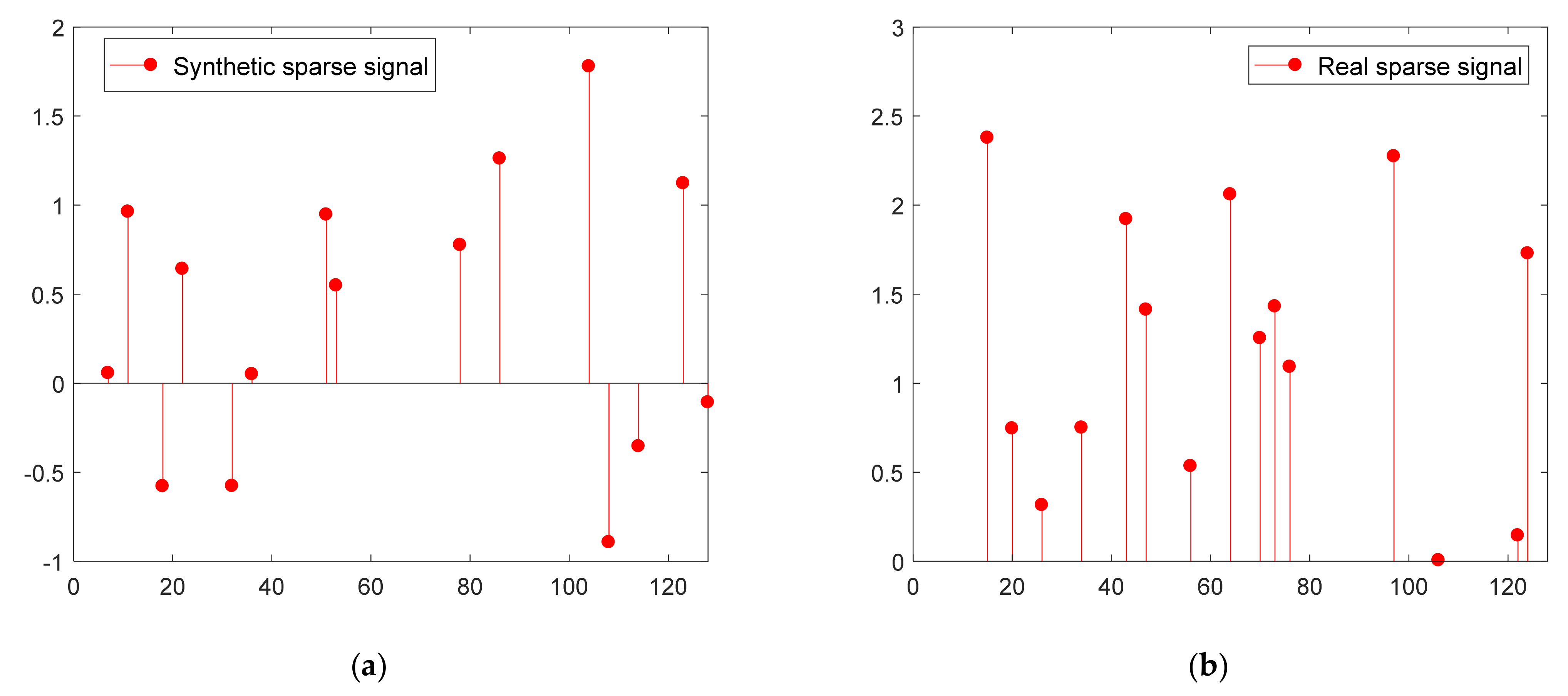
We evaluate the reconstruction performance of the proposed method using synthetic sparse data and real-world sparse data, respectively. Real-world data are non-negative voltage disturbance signals sampled from the vehicle power system, which are extraordinarily common impulse signals in this system. They are sparse in time domain, with approximately 10% of total elements nonzero. In order to give convenient explanation, values of all non-zero elements are normalized to [0, 1]. Therefore, the voltage disturbance signals can be represented as one-dimensional vectors.
Given the characteristics of real disturbance signals, we further generate Gaussian sparse data in a similar way. Specifically, suppose the one-dimensional sparse signal contains
K nonzero coefficients (
K is the sparsity level) with random locations. The nonzero coefficients are randomly generated with each entry independently drawn from a normalized Gaussian distribution. Synthetic sparse signals can be utilized as an essential supplement to real sparse signals to verify the completeness of FRSVssMP.
Figure 3a,b depict examples of one-dimensional synthetic signals and the original real signals, respectively, where we set the signal length equal to 128.
In this paper, essential experiments were conducted to illustrate superior performance of FRSVssMP against the state of the art algorithms including StOMP, CoSaMP, SAMP, AStMP [
20] and CBMP [
25]. Typical synthetic and real-world voltage disturbance signals from the vehicle power system were selected as trial data. Performance evaluation metrics includes reconstruction time and success rate. Reconstruction time
T in seconds refers to average time implemented for reconstruction. Reconstruction success rate is defined as the ratio of the number of successful trials to the total number of trials. To be specific, suppose
N is the signal length and
M denotes the length of measurement vector, then the root-mean-square (RMS) can be expressed as:
where
is the
originalsignal and
denotes the reconstructed signal. The successful trial refers to a trial with RMS less than 10
−6. In our simulations, each experiment was repeated for 5000 trials, and the sensing matrix
was generated as a zero mean random Gaussian matrix with columns normalized to unit
l2 norm. Experiments were implemented in MATLAB R2020a on Windows 10 (published by Microsoft, Redmond, America) with Intel Core i7 processor (3.6 GHz) with 4-GB RAM.
4.2. Performance of the Proposed Initial Sparsity Level Estimation Approach
Firstly, the proposed initial sparsity level estimation was evaluated in contrast to AStMP [
20], which shows the state of art performance in initial sparsity estimation. In this simulation, real signals were extracted with the length
N = 128. And the measurement length
M and sparsity level
K were fixed as
M = 64 and
K = 32, respectively.
Initial estimations of sparsity level in different experiments are shown in
Figure 4a. Performance of FRSVssMP and AStMP are compared with different
. The blue dotted line indicates the actual sparsity level (
). According to
Figure 4a, FRSVssMP achieves superior initial estimation of
K over AStMP as the estimated level is close to the actual level with the same
. In addition, by choosing an appropriate
, the initial estimation of
K will approximate to actual level obviously.
As illustrated in
Section 3, with the estimated sparsity level
k0, we set the initial step size to
for subsequent process. Further, to demonstrate the superiority of this setting,
Figure 4b demonstrates the estimated sparsity level obtained by different algorithms during iterations, with a focus on the selection of initial step size. Step size adaptively changes in different iterations, and finally, the sparsity level is accurately approximated. Taking advantage of the initial step size setting
, in contrast to SAMP, SASP and AStMP, FRSVssMP approximates the actual sparsity level more efficiently as the number of iterations required can be significantly reduced.
4.3. Reconstruction Performance versus the Sparsity Level
Then, we compared reconstruction performance of FRSVssMP with the existing algorithms versus the sparsity level K. In this simulation, for both synthetic and real sparse signals, signal length N and measurement length M were set to N = 256 and M = 128. And the parameters S, λ, α for FRSVssMP were set equal to , , throughout our experiments, where was the estimated initial sparsity level. The empirical results suggest that the step-size transformed parameter η is critical to the performance. For synthetic sparse signals, η was set to , while we set for real sparse signals.
4.3.1. Reconstruction Success Rates
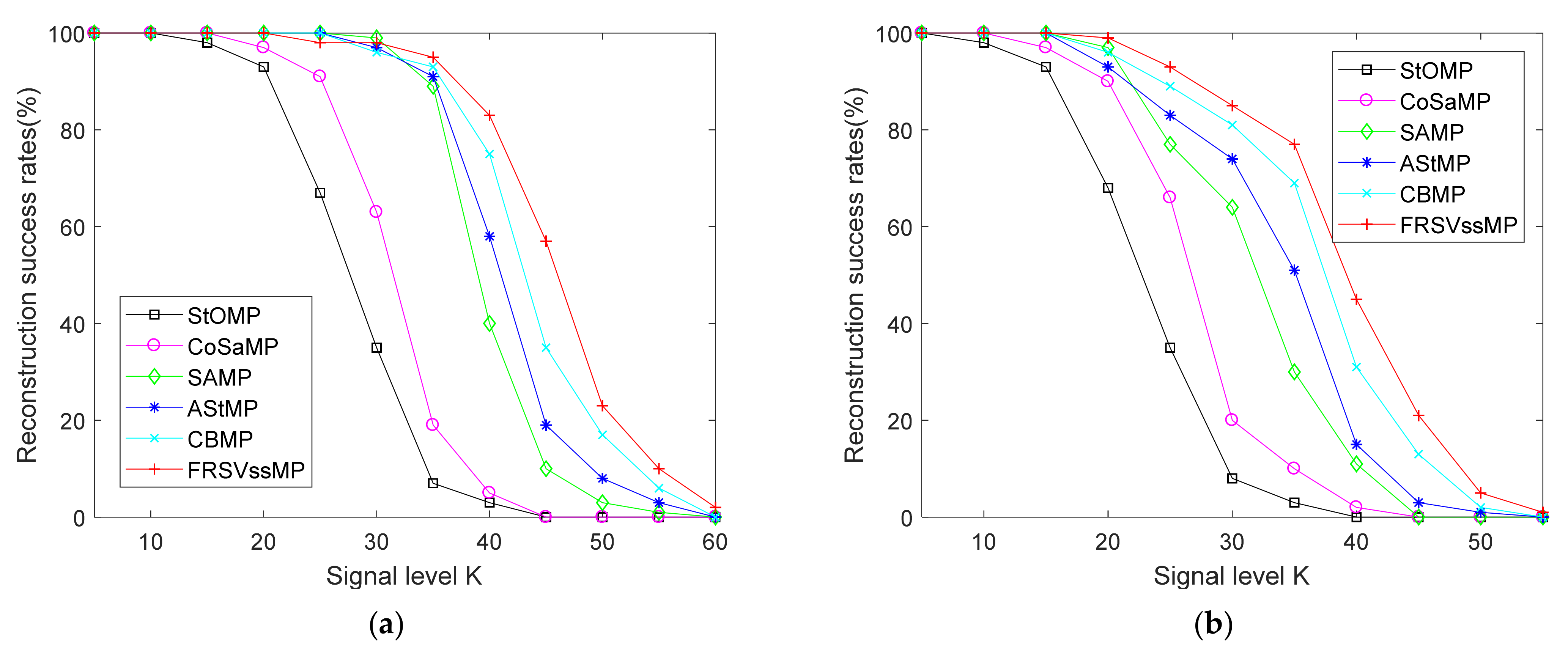
Figure 5a,b depict reconstruction success rates versus the sparsity level
K for synthetic and real signals. The horizontal axis represents different
K drawn from
, and the vertical axis shows the corresponding success rates (in percentages).
For a small K, high reconstruction success rates are acquired by FRSVssMP and the competing algorithms. As the sparsity level becomes large, success rates obtained decrease considerably, while differences between the success rates of the algorithms become significant. For both synthetic and real signals, FRSVssMP presents a considerable performance advantage over the greedy algorithms in the first category, such as StOMP and CoSaMP, due to the utilization of sparsity variable step-size adaptive. Moreover, FRSVssMP shows a slight superiority over SAMP, AStMP and CBMP on the whole, because it exploits the underlying information of the sparsity level and filters the incorrect atoms. CBMP acquires the second best performance, followed by AStMP, SAMP, CoSaMP, and StOMP.
4.3.2. Reconstruction Time
Figure 6a,b show reconstruction time versus the sparsity level
K for synthetic and real signals. The greedy algorithms in the first category were omitted since they took significantly longer time. The horizontal axis denotes the different
K drawn from
, and the vertical axis indicates the corresponding reconstruction time (in seconds). The initial step size selected according to the initial estimation approach may not work well in greedy algorithms with the fixed step size (such as SAMP). To make the comparison fair, we must evaluate reconstruction time with the similar success rates achieved by those algorithms. After a series of experiments, to ensure the similar success rates obtained by FRSVssMP, the step size was set to 5 for SAMP, and we also employed the appropriate parameters for CBMP.
It can be observed that, both for synthetic and real signals, compared with SAMP and CBMP, FRSVssMP performs better in terms of reconstruction time, which reveals that FRSVssMP is more efficient with the same sparsity level. This is due to the fact that, FRSVssMP selects a more appropriate initial step size by the initial sparsity level estimation approach and employs two stages of sparsity variant step sizes mechanism. Moreover, as sparsity level becomes larger, the reconstruction time increases. However, FRSVssMP shows better robustness as the amount of time increased for it is less compared to those for other algorithms, which means it works well for complex scenarios.
4.3.3. Performance of FRSVssMP and SAMP versus Variable Step Sizes
Additionally, to illustrate the influence of variable step sizes on reconstruction performance, FRSVssMP were compared with SAMP in different variable step sizes
S, i.e., 5 and 10.
Figure 7a,b demonstrate success rates versus variable step sizes for synthetic and real signals. The horizontal axis represents the different sparsity level, and the vertical axis shows the corresponding success rates (in percentages).
We can observe that, as sparsity levels become larger, the success rates decrease. For a small K, there is no significant difference among different variable step sizes in terms of reconstruction success rates. However, for a large K, as the variable step size become larger, the success rates decrease obviously. The reason for this lies in that a small variable step size approximates the actual sparsity level much more precisely. It can be concluded that, for both types of sparse signals, FRSVssMP achieves better success rates compared to SAMP with the same step size (5 or 10).
4.4. Reconstruction Performance versus the Measurement Length
In this subsection, we compared reconstruction performance of FRSVssMP with those of the competing algorithms versus the measurement length M. In this simulation, for both synthetic and real sparse signals, signal length N and sparsity level K were both set to N = 1024 and K = 20, respectively. Other parameters were set in the same way as in the previous part.
4.4.1. Reconstruction Success Rates
Figure 8a,b illustrate reconstruction success rates versus the measurement length
M for synthetic and real signals. The horizontal axis represents different
M, and the vertical axis shows the corresponding success rates (in percentages). For better comparison, the measurement lengths for synthetic sparse signals were drawn from
, while those were assigned to
for real sparse signals.
From
Figure 8, with the increase of the measurement length, success rates obtained grow considerably. Meanwhile, as
M becomes larger, the difference between reconstruction success rates calculated by different algorithms becomes more and more obvious. For both synthetic and real sparse signals, FRSVssMP outperforms all the greedy algorithms in the first category obviously, especially with a large
M. FRSVssMP makes a more accurate estimation of the sparse signals by the initial sparsity level estimation approach as a result of the increasing information acquired from the measurement vectors. FRSVssMP performs better for almost all measurement lengths compared to AStMP and CBMP because of the accurate initial sparsity level estimation along with the filtering mechanism. As the nearest rival to FRSVssMP, CBMP shows superiority over other algorithms with two kinds of composite strategies, followed by AStMP, SAMP, CoSaMP, and StOMP.
4.4.2. Reconstruction Time
Figure 9a,b depict reconstruction time versus the measurement length
M for synthetic and real signals. Similarly, in this experiment, the greedy algorithms in the first category were omitted because that they took considerably longer time. The horizontal axis represents different
M, and the vertical axis shows the corresponding reconstruction time (in seconds). For better comparison, the measurement lengths for synthetic signals were drawn from
, while those were assigned to
for real signals. To ensure similar success rates obtained by FRSVssMP, the step size was set to 4 for SAMP, and the appropriate parameters were selected for CBMP.
As can be seen from
Figure 9, for both synthetic and real sparse signals, reconstruction time achieved by FRSVssMP is less than that of SAMP and CBMP for different measurement lengths. This implies that, FRSVssMP is more efficient than the competing algorithms with the same
M because of the initial sparsity level estimation approach and sparsity variable step-size adaptive mechanism. In addition, FRSVssMP shows superiority in terms of robustness as the range of the reconstruction time for it is less than those for the competing methods.
4.4.3. Performance of FRSVssMP and SAMP versus Variable Step Sizes
To illustrate the influence of variable step sizes on reconstruction performance, FRSVssMP were compared with SAMP in different
M.
Figure 10a,b demonstrate success rates versus variable step sizes for synthetic and real sparse signals. The horizontal axis represents different
M, and the vertical axis shows the corresponding success rates (in percentages). To make the comparison clearer, FRSVssMP was compared with SAMP in different variable step sizes for synthetic and real sparse signals.
We can find that, for different M, there is not much difference in reconstruction success rates between different variable step sizes. As the variable step size grows, the success rates decrease slightly since that a small variable step size approximates the actual sparsity level much more easily. It can be concluded that, for both types of sparse signals, FRSVssMP has advantage over SAMP in terms of success rates with the same step size.
5. Conclusions
With the explosive growth of ubiquitous vehicles, CS has been widely employed in signal sensing and compression in vehicle engineering. This paper firstly introduces an initial estimation approach for the signal sparsity level, then proposes a novel greedy reconstruction algorithm, i.e., FRSVssMP, for real-time vehicle health monitoring. The proposed algorithm first selects an appropriate initial step size by the initial sparsity level estimation approach. Then it integrates strategies of regularization and variable adaptive step size, and further performs filtration. Relying on no prior information of the sparsity level, FRSVssMP could achieve an excellent reconstruction performance. FRSVssMP is applicable for scenarios requiring high reconstruction accuracy and efficiency, especially in vehicle health monitoring. Since various faults exerts serious impact on the operation of vehicles and even lead to traffic accidents, health monitoring for vehicles has extremely high requirements. FRSVssMP can promote the reconstruction accuracy and efficiency for status data obviously, which can be beneficial for the subsequent analysis and diagnosis.
Simulation results demonstrate that, taking typical voltage disturbance signals in vehicle power system disturbance monitoring as trial data, the proposed FRSVssMP outperforms the state-of-the-art greedy algorithms both in terms of reconstruction success rates and time. Furthermore, we demonstrate that the reconstruction performance of the greedy algorithms is highly relevant to variable step sizes. During the iterations, some parameters, i.e., an initial step size, an iteration-terminating parameter, a step-size transformed parameter, and a step-size adaptive parameter, have critical influences on the reconstruction. How to scientifically select appropriate values for these parameters will be the subject of our future work.


