1. Introduction
Stability in a traditional continuous dynamic system is a property related to robustness and resilience, and designing a system to have this property is an essential issue of system control and design [
1]. A stable system can eventually converge the desired steady state from an arbitrary state. To rephrase, a system can recover its original state even if it has left the steady state because of an exception or abnormality. Although stability has been introduced for continuous systems, discrete event systems, such as manufacturing systems or computer networks, also have similar stability issues such as boundedness, practical stability, and Lagrange stability in the sense of Lyapunov stability or asymptotic stability [
2]. A general Petri net, a kind of a discrete event system modeling language, usually analyzes structural boundedness, a special case of Lagrange stability [
3]. In that sense, the event graph, also known as a marked graph, is always a bounded Petri net, so it is stable at all times. Therefore, an event graph is rarely necessary to analyze the system’s boundedness, but it is useful for modeling a cyclic schedule for mass production, thanks to this stability [
3,
4,
5].
However, some cyclic production systems have another type of stability issue even after modeling with event graphs. For example, a cluster tool for chemical vapor deposition (CVD) has a lower time limit, which is the minimum time required to perform a task, as well as an upper limit of wait time until the next task. The constraint forces a cluster tool to regulate fluctuations of delay or wait time between tasks to keep the product quality uniform and predictable. We call this constraint a time window constraint. Many researchers have studied how to model the cyclic schedule of a cluster tool with deterministic time using a timed event graph (TEG) to satisfy the constraint [
6,
7]. A TEG is a Petri net that temporizes by introducing the concept of deterministic time to places in an event graph. However, an existing system has persistent time variations or exceptions, so a TEG model analysis result cannot sometimes reflect the real one. Therefore, some studies have considered the predictable time fluctuation range when modeling and analyzing schedulability using the modified TEG [
8] or have suggested a method of controlling the system within the time constraint [
9].
Nevertheless, if rare exceptions occur such as time fluctuations more significant than expected or abnormality, we must quickly enable the system to converge to its normal state. Analyzing a discrete event system’s stability with such time constraints determines whether each task has asymptotically reached desired steadiness that repeats it at fixed intervals rather than analyzing the boundedness. In other words, a system that is not stable does not repeat each task at the same time interval. However, even an unstable cyclic discrete event system repeats a pattern with the time interval. We call the analysis of temporal patterns
cyclicity analysis [
3,
10,
11].
Some researchers have analyzed the cyclicity and stability with regard to the time interval pattern of TEG [
3]. Specifically, if each transition repeats firing epochs asymptotically every time a specific integer
d-cycles, the system is considered
d-cyclic, and the one-cyclic system is considered stable. However, it is not intuitive to analyze cyclicity and stability in a TEG. Therefore, these researchers have modeled a system with a TEG and converted it into a matrix form of (max,+) algebra [
8,
11,
12,
13]. (max,+) algebra is an idempotent semiring of extended real numbers
that can model and analyze the concepts of synchronization and concurrency [
11,
14,
15,
16,
17]. It also has a concept of stability like the one we have explained here, so it is easy to analyze the periodicity and stability of the system [
10,
18,
19]. However, it is not intuitive to model the dynamic behavior of the system directly with (max,+) algebra, so the analysis is performed by dualizing TEG for modeling and (max,+) algebra for analysis. Two-step analysis itself is complicated, but interpreting a (max,+) algebra model in light of the original discrete event system is also not intuitive, making improving system stability difficult.
This article uses the idea that the final result of the matrix form of (max,+) algebra for analyzing the stability is also another TEG with specific characteristics: for instance, every place has exactly one token and at most one place connecting two transitions. We first provide equivalent transformation rules between TEGs without using (max,+) algebra including place reduction rules [
20] and token simplification [
10]. Then, using these rules, we propose a methodology to analyze stability and cyclicity in terms of a TEG. In conclusion, we provide a direct way to calculate an asymptotic cyclicity of a given TEG and to determine whether the TEG is stable without any conversion.
This article is organized as follows:
Section 2 is devoted to introducing various notations, preliminary TEG concepts, and (max,+) algebra. It also illustrates how to analyze the cyclicity and stability using a two-step analysis.
Section 3 presents rules for changing to an equivalent TEG with the characteristics of a precedence graph without converting a given TEG into a matrix form. In
Section 4, we suggest theoretical background finding cyclicity and stability at the TEG level. Finally, we conclude in
Section 5.
3. Transformation from a TEG to Its Precedence Graph
This section explains how to transform a general TEG into a precedence graph without going through converting the (max,+) algebra to a matrix form. The precedence graph defined in
Section 2 is a special type of TEG with three properties as follows [
10]: There is at most one token in each place, there is always a token in all places, and there is only one place that directly connects any two transitions. Therefore, to convert from a general TEG to a precedence graph, we must separate the place with multiple initial tokens into as many places as the number of tokens, remove a place without a token by concatenation with another place, and merge parallel places that directly connect two transitions into one place.
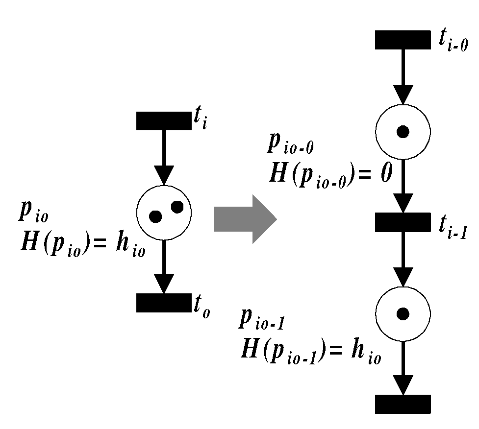
First, we explain how to remove the place with multiple tokens so each place has at most one token. There already exists a method of transforming a place with multiple tokens to another equivalent TEG [
10]. Specifically, when a TEG has a place with multiple tokens, as in
Figure 4, we can construct another TEG with the corresponding places with at most one token in the initial marking.
Rule 1. Concatenation of sequence places
- Precondition:
A TEG if there exists a place that initially has more than one token ().
- Rule:
A transformed equivalent TEG , such that
- 1.
, where
- 2.
, where
- 3.
- 4.
- 5.
- 6.
- 7.
- 8.
if , otherwise
We illustrate Rule 1 with
Figure 4. Steps one and two describe how sets of places and transitions are changed. Place
, with multiple tokens on the left of
Figure 4, is replaced with as many new places as the number of initial tokens (i.e., two places with one token,
and
). Transition
is also divided into
and
. Step three guarantees that each new place has exactly one token. Steps four through seven explain how to connect
and
. The last step defines the holding time of new places. The holding time of the place
in the original TEG is allocated to
, and directly connected to the transition
. The holding time of the remaining new places is zero. If we apply this rule to all places with multiple initial tokens, the number of places and transitions increases, but it is known that the new TEG becomes equivalent to the original TEG. To sum it up, the firing epochs of the surviving transitions and the number of tokens between them do not change.
We now describe removing the place
p with zero tokens from a TEG by concatenating it to another place. Because a live event graph always has the upstream transitions, the transitions belonging to
may disappear at the same time. However, we assume that the TEG operates using the earliest starting strategy, and so the firing epoch of the removed transition is calculated automatically from the epochs of the remaining transitions. Therefore, the transformed TEG has the same dynamic behavior as the original, so they are equivalent. There are two rules for removing a zero-tokened place, depending on how many downstream places the
has: Rules 2 and 3. First, if
as in
Figure 5, the upstream transition
in the removed place
has only one downstream place,
itself, Rule 2, as inspiration from the serial fusion rule [
20], can be applied.
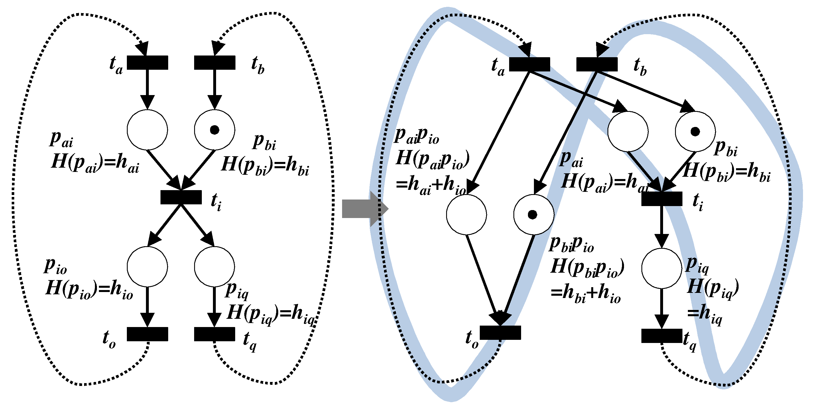
Rule 2. The case in which both a place with a token and its upstream transition are removed.
- Precondition:
When a TEG has Place , which has no initial token, we assume that its upstream and downstream transitions are and , respectively, and has only one downstream place ()
- Rule:
A transformed equivalent TEG such that
- 1.
, where
- 2.
- 3.
- 4.
- 5.
- 6.
Figure 5 shows an example in which place
without any token is concatenated to
, and its upstream transition
is removed. As a result, the number of places and transitions of the new equivalent TEG decreases by one. The new place is named
and
in succession, with two concatenated places’ names, and their initial markings are the same as
and
, respectively. Their holding times are the sum of two holding times of the merged places (i.e.,
and
). Lemma 1 proves that the TEG derived by Rule 2 is equivalent to the original TEG.
Lemma 1. TEG derived by Rule 2 is equivalent to .
Proof. The set of transitions of TEG
newly derived by Rule 2 is
, which is a subset of the original transition set. We denote the
rth firing epoch of the transition
as
and then assume that place
has no initial token. That is,
at the
rth firing epoch of
. The
rth firing epoch of
of the newly created TEG
is changed to
If firing epochs of transitions other than are the same, the two TEGs are equivalent by Definition 1, given that the number of tokens between the remaining transitions and firing epochs of do not change. □
The next rule removes zero-tokened
, whose upstream transition
has multiple downstream places. After applying this rule, a place without a token in the original TEG is concatenated to the preceding places
, but the upstream transition
does not disappear.
Rule 3. The case in which a place with a token is removed, but its upstream transition survives.
- Precondition:
When a TEG has Place , which has no initial token, we assume that its upstream and downstream transitions are and , respectively, and has multiple downstream places, unlike Rule 2 ().
- Rule:
A transformed equivalent TEG such that
- 1.
, where
- 2.
- 3.
- 4.
- 5.
- 6.
.
Rule 3 is similar to Rule 2 in that a place without a token is concatenated to the upstream places of its upstream transition, but its upstream transition has other downstream places, so it is making the two rules different in that the transition survives after applying the rule.
Figure 6 shows an example in which place
is replaced with
and
according to Rule 3. This example does not remove the upstream transition
of
, as opposed to Rule 2. The number of transitions of both TEGs before and after applying the rule is the same as five, but the total number of places increases by the number of upstream places of
. The holding times, the initial markings, and the naming convention of transformed places are the same as those in Rule 2. Lemma 2 proves that the TEG after applying Rule 3 is equivalent to the original TEG.
Lemma 2. TEG derived by Rule 3 is equivalent to .
Proof. The set of transitions of TEG transformed by Rule 3 is the same as the original transition set except for the connection relationship with the place. The rule does not change any of the downstream places of the upstream transition of place by Rule 3 except and , so has the same firing epoch after applying the rule. fires at the same time as before the rule was applied for the same reason as in Lemma 1. In addition, the initial marking of the new place , where , so the number of tokens between and has not changed. That is, the transformed TEG from applying Rule 3 is equivalent to the original TEG. □
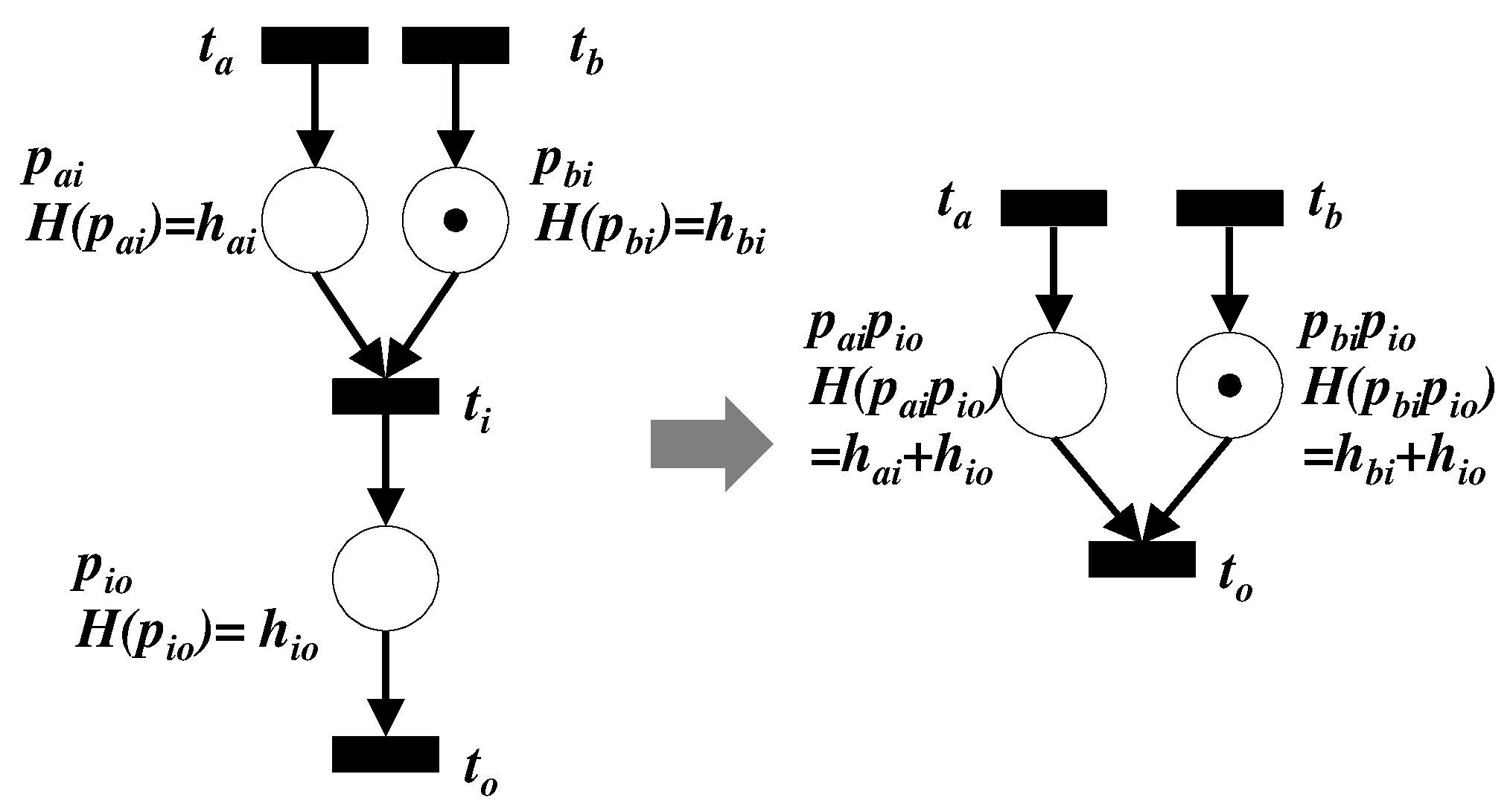
Finally, we examine the case in which merging multiple places with the same number of tokens connecting two consecutive transitions into one, as shown in
Figure 7. We can apply Rule 4 for this case.
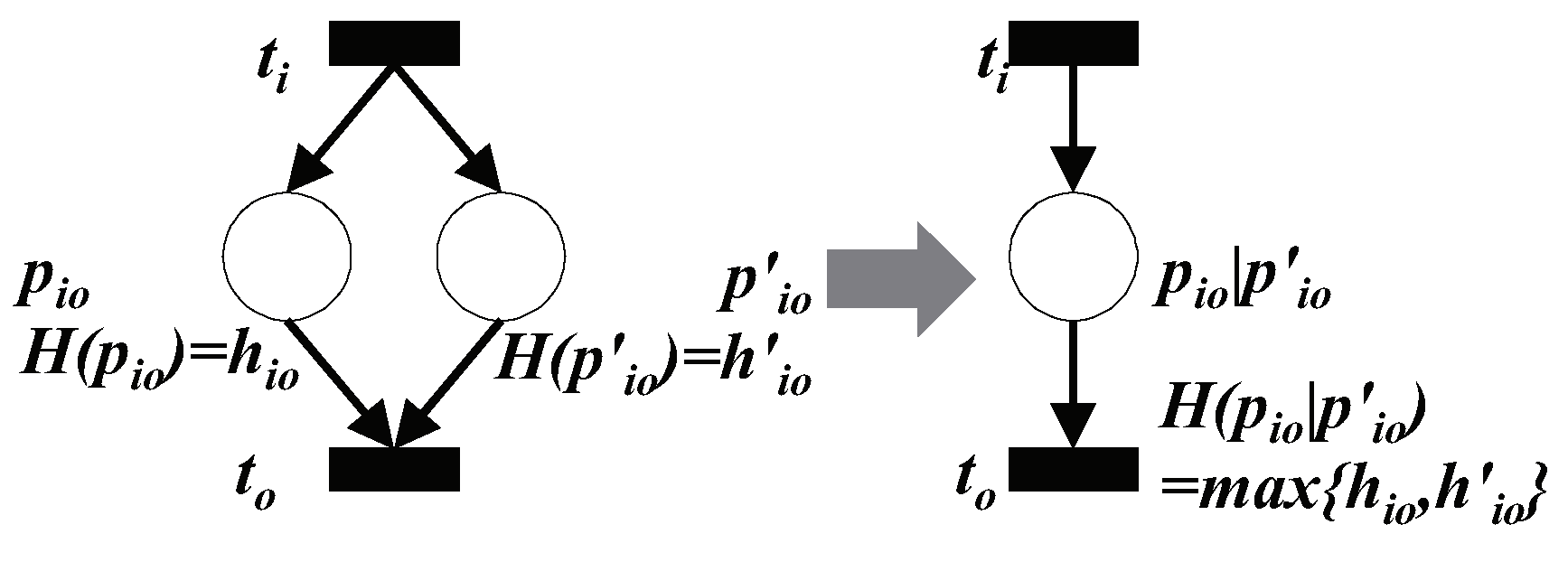
Rule 4. Merging of parallel places.
- Precondition:
There is an arbitrary subset S of places in which the initial token number, the upstream transition and the downstream transition of all places belonging to S are the same.
- Rule:
All places belonging to the set of places S may be replaced by a single place, specifically a transformed equivalent TEG such that
- 1
- 2
- 3
- 4
- 5
.
By way of explanation, if we apply Rule 4, the new place’s holding time is the maximum of the original places, and its upstream transition and downstream transition do not change. We denote | notation to indicate which places are merged in the place newly created by Rule 4 when parallel places directly connect two transitions.
Figure 7 illustrates how zero-tokened places
and
, which directly connect
and
merge to form
. Its holding time becomes the maximum value of the holding time of
and
. Lemma 3 proves that the new TEG after this transformation is equivalent to the one in existence before the application of Rule 4.
Lemma 3. TEG transformed by Rule 4 is equivalent to .
Proof. When all places connect from
to
and have the same number of tokens, we call them parallel places, and their set is denoted as
S (
). All places included in the set of the upstream places of
but not belonging to
S is denoted as
(
). Under this assumption, the
rth firing epoch of
after applying Rule 4 is changed from Equation (
6) to Equation (
7):
If the firing epochs of the other transitions except for are the same as before, the firing epoch of is also the same. Therefore, by Definition 1, the TEGs are equivalent. □
This paper proposes four rules to simplify the equivalent TEG. If we repeatedly apply the transformation rules proposed in this paper, we can finally derive a TEG equivalent to the original TEG to satisfy the properties of the precedence graph. We have already proved that a transformed TEG is always equivalent even after applying any of Rules 1–4. Therefore, we now show that repeatedly applying rules can make a TEG eventually satisfy the precedence graph’s properties. In other words, every place has exactly one token in the final TEG, and the number of places directly connecting any two transitions is at most one. To prove that every place has exactly one token, we first show that any place has at most one token by contradiction. In other words, we hypothesize that there remains a place with two or more tokens no matter how often the rule is applied. In this case, we can decrease the number of tokens to one by applying Rule 1 to a place with multiple tokens. This decrease violates the hypothesis that, no matter how much the rule is applied, a place with multiple tokens cannot be removed. Therefore, we can always make the number of tokens fewer than one in all places. Next, we prove that there is at least one token in every place. The event graph, which this paper considers, is autonomous, so every place has its input transition. Therefore, we prove that every place has at least one token by showing that every transition has only its downstream places with tokens. When there is a transition with a downstream place without tokens, we divide the cases by the number of its downstream places. If the transition has only one downstream place without tokens, we can remove the transition using Rule 2. After that, a TEG has no transition, whose downstream place has no token. If the transition has multiple downstream places, we can remove a downstream place without tokens by applying Rule 3. If the transition has multiple downstream places with no tokens, we can remove them by applying Rule 3 repeatedly until every downstream place has at least one token. This way, we can make sure every place has at least one token. Finally, we prove by contradiction that there is at most one place that directly connects two arbitrary transitions. Expressly, we assume that no matter how many times rules are applied, there still remain multiple places that directly connect two transitions. We can make the number of tokens in those places at most one by Rule 1. If a place with more than two tokens exists, it does not link directly between the transitions because the place is replaced with a series of other places and transitions. Next, places that connect directly connected transitions are merged according to the number of tokens by Rule 4. After applying Rule 4, if the places are merged into one, the assumption that we cannot merge places between two transitions into one is violated. If there are two places, one place has a token and the other has no token. Rule 3 can make it so there is only one place between the transitions by removing the place without tokens, so this situation also violates the assumption. Therefore, we can make a TEG in which every pair of transitions is connected by one place at most. In conclusion, if we apply Rules 1–4 repeatedly to a live autonomous TEG, we can achieve a TEG equivalent to the original and eventually have the properties of a precedent graph.
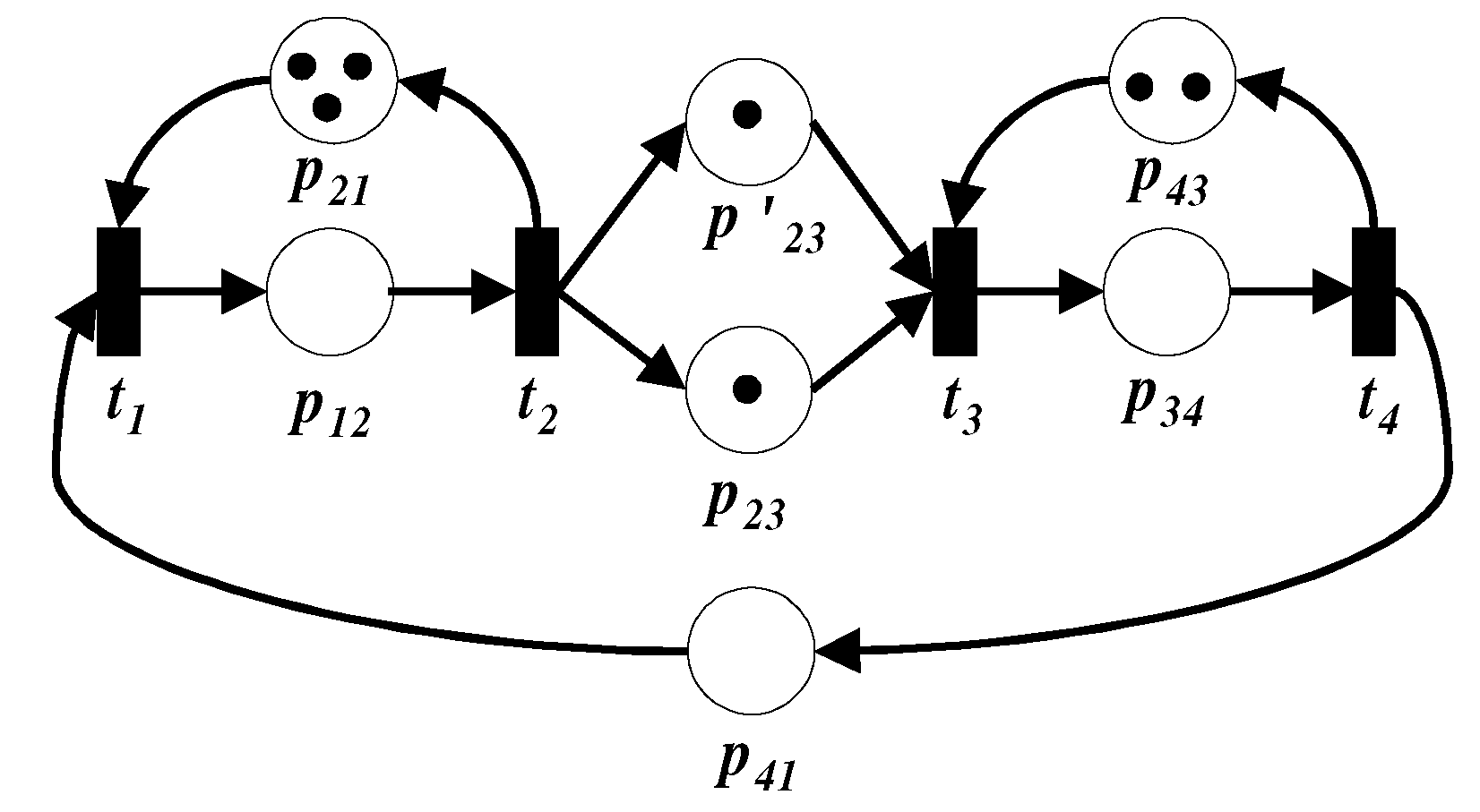
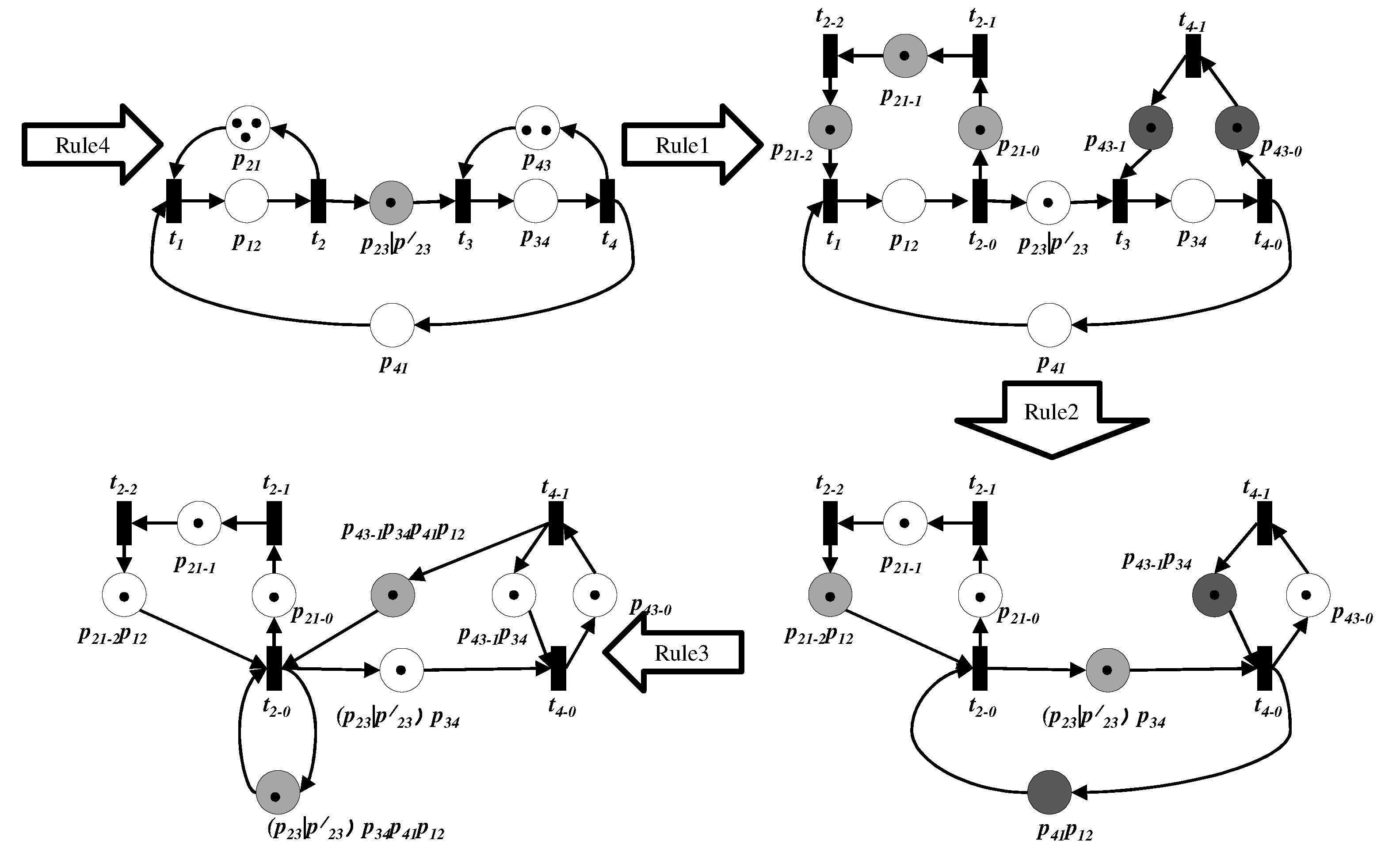
Figure 8 illustrates the process of deriving a precedence graph from
Figure 1 while repeatedly applying transformation rules. For better understanding, the newly created place in each step is highlighted in gray. First, parallel places
and
are merged using Rule 4. In the next step, places with multiple tokens
and
are divided into corresponding places by Rule 1: (
,
and
) and (
and
). Now, there are currently three places without tokens,
,
, and
, so we must remove them using Rules 2 and 3. The upstream transition of each of places
and
has only one downstream place, so Rule 2 is applied. For
, the upstream transition
is removed, and the place
is concatenated to
and
, which belong to the upstream places of
. Like
,
is concatenated with
and
by removing Transition
. Now, there only remains one place without tokens,
. Its upstream transition is
, which has two downstream places,
and
. After Rule 3 is applied, two new places are created by concatenating
with the upstream places of
,
and
, respectively. The TEG in the last step of
Figure 8 has the precedence graph’s properties and is isomorphic with the precedence graph in
Figure 2.
4. Stability Analysis of a TEG
This section analyzes how the original TEG
properties affect the derived precedence graph
and suggests how to calculate the cyclicity of a live autonomous TEG. First, we investigate which transitions of
become corresponding vertices or decompose into multiple corresponding vertices. Lemma 4 determines which transition survives as the vertex of
.
Lemma 4. If and only if a transition of TEG has at least one downstream place with a token, the transition has corresponding vertices in .
Proof. To prove this lemma, we show that, if any downstream place has a token, we cannot remove its upstream transition, and if there is no place with a token among the downstream places, the transition is always removed.
First, we prove that a transition whose downstream places have tokens is not removed. Only Rule 2 eliminates a transition after applying the rule. The precondition of the rule is that there is no token in the downstream place of the transition. Even when the downstream transition of its downstream place has been previously eliminated, the token cannot exist in the new downstream place because it occurs only as a result of Rule 2, so the place does not have a token. Therefore, a corresponding transition exists in the precedence graph derived by repeatedly applying transformation rules when one or more downstream places have tokens.
Next, we show that the transition without a token in the downstream place is finally not included in the precedence graph. If all downstream places of a transition have no tokens, Rule 3 is applied repeatedly until only one downstream place is left, and then the transition can be eliminated using Rule 2. Therefore, a transition whose downstream places have no tokens is eventually removed. □
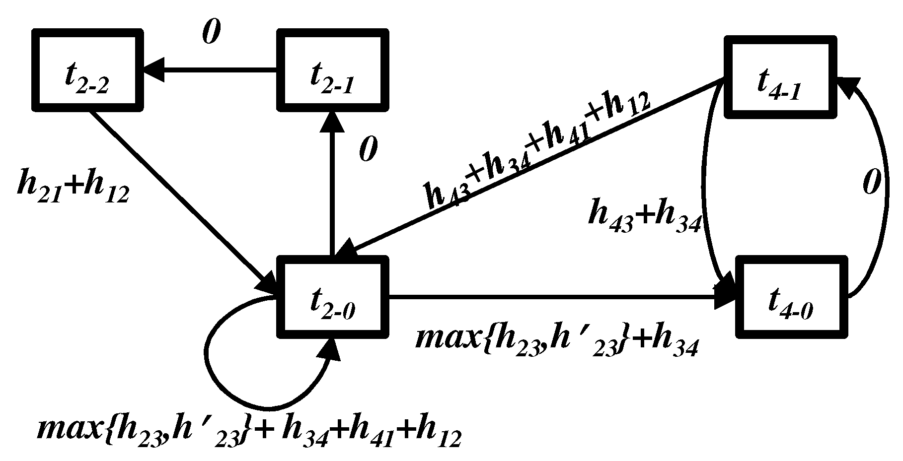
For example, let’s check how to map the transitions of TEG
in
Figure 1 to the vertices of precedence graph
in
Figure 2. The only transitions with tokened downstream places are
and
in the TEG
, and their corresponding vertices are as follows:
(
,
and
), and
(
and
). In other words, only the corresponding vertices of
and
of the precedence graph have downstream place tokens.
Next, we examine the view of the cycle. Because a live autonomous TEG has a token for each cycle, at least one transition survives as a corresponding vertex for each cycle. In this example, the cycles
and
of
go through both
and
, and the cycles
and
go through both
and
. Looking at the corresponding transition of the vertex included in each cycle of
, cycles
and
have only
, and
is related to
. Cycle
is related to both
and
. Then, what is the relationship between the cycles of
and
? Lemma 5 investigates the relationship between the two.
Lemma 5. If a cycle exists in the original TEG , a corresponding cycle exists in the derived precedence graph . If there is a cycle in the derived , there is a corresponding cycle and concatenation of corresponding cycles in .
Proof. We prove this lemma by observing how each rule changes a cycle based on how reachable the transition is. That one transition is reachable from another means that a path exists between them.
First, we prove that Rule 1 does not change the reachability among transitions. According to the rule, the corresponding transitions of denoted as are reachable from by 5–8 of Rule 1. Additionally, only transitions having a path to have a path to and vice versa because the sets of upstream places of and are the same. For the same reason, a transition is reachable from after applying the rule if and only if it is reachable from before doing so. From the point of view of a cycle, if belongs to a particular cycle before applying the rule, its corresponding transitions belong to the corresponding cycle. In other words, Rule 1 does not change the transition’s reachability, so we can find the corresponding cycle of any cycle after applying the rule. This rule does not change the number of tokens or the cycle times either. Although the number of places increases by the number of tokens, the number of tokens in the newly created place is one for each, so the numbers of tokens of both TEG are identical. The sum of the holding time of the corresponding cycle is not changed because this rule decomposes one place into multiple places, but only one place has the same holding time as the original place , and the rest of the places have zero holding times for a positive integer j that is smaller than . As a result, the number of cycles does not change after applying Rule 1, and the cycle time of the corresponding cycles is the same as the original cycle times.
Rule 2 also does not change reachability, except for the direct connections of and caused by the removal of . Therefore, the sets of transitions reachable to and reachable by do not change, so the reachabilities between surviving transitions remain. From the viewpoint of the cycle, the cycles including for the transitions in directly connect to after applying Rule 2. The cycle has the same cycle time and sum of tokens as the original because calculates the value by summing tokens of concatenated places and where belongs to . In summary, Rule 2 does not change the number of cycles or the cycle time of each cycle.
After applying Rule 3, the directly connected path from
to
disappears when the place
is removed. The result excludes
in the cycles that include both
and
initially. This removal divides the cycles formerly including
into two kinds of cycles: cycles including the new place that directly connects
to
and the unchanged cycles that still include
. Additionally, this rule creates new cycles that concatenate these two types of cycles not to pass the same arc or transition except for
. In other words, we build a new cycle by connecting two different kinds of cycles after switching the upstream place of
in two cycles. Therefore, the total holding time and number of tokens of the created cycle are the sums of the data for two connected cycles. To help understand the proof, we illustrate how Rule 6 increases cycles using
Figure 6. In the figure, the dotted line and the gray line denote the arbitrary path to create a cycle and the newly created cycle, respectively. Assume that
and
belong to
and
and
are in
, where
is not
and
is also not
. The left TEG has two cycles with
and
, which share no transition except
. The right TEG has an additional new cycle connecting them in the following way: decrease the cycle in the sequence of
, the new place
,
, the path removing
from the cycle including
and
(
), and the path removing
from the cycle including
and
(
).
Rule 4 does not change transitions. It merges places whose upstream transition, downstream transition, and token number are identical. Given that these merged places have the same upstream transition and downstream transition, the reachability does not change. That is, if and only if there was a cycle that a merged place could make with , all other merged places also make a cycle use the same path. We can also compose a cycle using the new place with the same path. Thus, if the original TEG has cycles because there are m different paths from to and n places are merged by Rule 4, the number of cycles decreases to m after the rule is applied. The cycle time of transformed TEG becomes the maximum cycle time of n merged cycles. The number of tokens in the corresponding cycle does not change. □
We can now comprehend the meaning of the proof of Lemma 5 using
Figure 8. The first step merges places
and
by applying Rule 4, so the cycles
and
are combined into one cycle. The cycle time of the combined cycle is the same as the maximum of cycles
and
, and its token numbers are unchanged. Other cycles
and
remain, so the number of cycles decreases to three. The next step decomposes the corresponding transitions from
and
by Rule 1. Consequently, cycles
and
increase the number of transitions and places, but the transformed TEG keeps the cycles and cycle times. The third step removes the places
and
using Rule 2. Cycle
becomes
, each of whose places has exactly one token. Cycle
still keeps the number of tokens and the sum of the holding times of places that make up the cycle, so the cycle times of
and
are the same. Similarly,
becomes
, and their cycle times are equal. In the final step, applying Rule 3 causes the place
to disappear. As a result, we can remove all zero-tokened places in the combined cycle from the first step, and we call it
.
The cycle time of
is still the maximum of
and
, and the number of tokens is maintained as one. Additionally, this step creates a new cycle
by connecting
and
. The newly created
has the cycle time of the sum of the maximum cycle time of cycles
and
plus
. Its number of tokens is three, which is the sum of the number of tokens in the connected cycle
and
. As such,
Figure 8 satisfies Lemma 5. From the proof of Lemma 5, we can also derive Collarories 1–3.
Corollary 1. If a cycle of a precedence graph corresponds to one cycle π of the original TEG , its length is the same as the number of tokens of π. By comparison, if a cycle is the concatenation of more than two cycles , its length equals the sum of the number of tokens in .
Corollary 2. If a cycle of a precedence graph corresponds to one cycle π of the original TEG , the sum of the holding times of the places it comprises is the same as the sum of the holding times of the places that make up π. If is derived from the concatenation of multiple cycles , the sum of the holding times of all places constituting equals the holding times of the places included in . However, if there are places merged by Rule 4 among , only the maximum value is added without adding their individual values.
Corollary 3. Rules 1–4 do not change the reachability between transitions.
Proof. Lemma 5 shows that the reachability is unchanged except in the case of Rule 3. Rule 3 eliminates the place directly connecting from , so we suspect that may no longer reach . However, given that every transition in a live autonomous TEG is included in any cycle, has a path to , and can connect to via new places. Therefore, there is a path, new place . In conclusion, Rule 3 also does not change the reachability. □
It is known that the stationary behavior is
d-cyclic if the transitions of a strongly connected TEG fire under the earliest starting strategy [
3]. From the lemmas and corollaries proved thus far, we can find the cyclicity in a live autonomous TEG as Theorem 1.
Theorem 1. When a live autonomous TEG is strongly connected, the cyclicity of a TEG is the LCM of the cyclicities of all maximal strongly connected subgraphs of , which is a critical graph consisting only of critical cycles. The cyclicity of each maximal strongly connected subgraph of is the GCD of the number of tokens of all its cycles. In other words, if the cyclicity of a TEG is d, it has an asymptotic d-cyclic schedule, and, if it is an asymptotic one-cyclic schedule, this system is said to be stable or to have stability.
Proof. Definition 2 said that the one-cyclic schedule is stable, so this proof focuses on whether the TEG’s cyclicity calculation is correct. Additionally, it is known that the asymptotic cyclicity of a strongly connected precedence graph
can be calculated by the LCM of the cyclicities of all maximal strongly connected subgraphs of its critical graph
[
10]. The cyclicity of each strongly connected subgraph of
is the GCD of the number of arcs of all its cycles. Therefore, we prove this theorem in the following order:
- 1.
If and only if there exists a critical cycle in , there exists a corresponding critical cycle and/or a connection of the corresponding critical cycles in .
- 2.
and belong to the same component of if and only if the corresponding cycle of and and their connection in also belong to the same component.
- 3.
The GCD of the number of tokens of all its cycles in each maximal strongly connected subgraph of is the same as the GCD of the number of arcs of all its cycles in each maximal strongly connected subgraph of .
1. First, we prove that has a critical cycle if and only if its corresponding cycle is critical and the cycle including it is critical in . A critical cycle is a cycle that has the maximum cycle time, calculated by the sum of the holding times of the places divided by the number of tokens in the cycle. The number of tokens and the sum of holding times of each cycle remain after the transformation, according to Corollaries 1 and 2 with the exception of Rule 4. Even Rule 4 does not change which cycle is critical because the cycle time after the transformation depends on larger cycle times among merged cycles by applying Rule 4. In other words, if a merged cycle is one of the critical cycles, its cycle times affect the cycle time after the transformation, so the corresponding cycle also becomes critical. Using this fact, we prove that the critical cycle of is the corresponding critical cycle of or a concatenation of the critical cycle.
Assume that corresponds to one cycle in . In addition, suppose that the critical cycle of is not the corresponding cycle of the critical cycle of . The cycle does not disappear even after rules are applied. Therefore, there is always a cycle in corresponding to cycle . Similarly, has a corresponding cycle of a critical cycle in . Because is critical, its cycle time is greater than or equal to the cycle time of the corresponding cycle of . Cycle is critical in the precedence graph, so the cycle time of is greater than or equal to the corresponding cycle time of . Remember that the cycle time and the number of tokens are unchanged after the transformation. For both to be true, the cycle time of and must be the same: that is, if and only if is critical for and corresponds to one cycle in , the corresponding cycle is also critical for .
Next, assume that
is a connection of the cycle
and
in the original TEG. We denote the sums of holding times of
and
as
and
and their token numbers as
and
, respectively. Suppose
without losing generalization and that the critical cycle of the original TEG is
. Its holding time and the number of tokens are
and
, respectively. Given that the corresponding cycle of
exists in the precedence graph and
is a critical cycle, the following inequality holds:
Cycle
is one of the critical cycles in the original TEG, so
and
. For both this inequality and Equation (
8) to be established at the same time,
, so
must be true. That is to say, if the critical cycle
is the connection of the cycles
and
in the original TEG,
and
are also critical cycles in the original TEG, and their cycle times remain.
Finally, we prove that, if corresponds to the connection of and , which are critical in , is also a critical cycle of . The critical cycle of is the same as the cycle time of the original TEG in the previous proof. Because and are critical together, . Therefore, the cycle time of is is the same as the cycle time of and . In conclusion, if critical cycles’ connections exist in the form of cycles in the precedence graph, they are also critical cycles.
2. Corollary 3 says that the reachability of cycles of the original TEG stands up in the precedence graph. Therefore, if and only if any critical cycle and belongs to the same component in , their corresponding cycle or existing connection of corresponding cycles belongs to the same component in .
3. The cyclicity is the LCM of the cyclicity of all maximal strongly connected subgraphs of subgraph
. Remember that each maximal strongly connected subgraph’s cyclicity is equal to the GCD of the arc number of each cycle constituting the subgraph [
10]. All maximal strongly connected subgraphs of
have the corresponding connected subgraph of
. The number of arcs of each cycle constituting the subgraph in
is the same as the number of tokens in its cycle in
. Therefore, the GCD of the number of arcs in
can be interpreted as the GCD of the number of tokens of the original TEG. Although the maximal strongly connected subgraph of the precedence graph has not only the critical cycle but also the connection to the critical cycle, the existence of cycles that exist in only
does not affect the GCD because
by the Euclidean algorithm. A TEG
’s cyclicity is the LCM of the cyclicities of all maximal strongly connected subgraphs of its critical graph
. □
Theorem 1 lets us know that the cycle times of
,
,
and
in
Figure 1 are
,
,
, and
, respectively. If
or
is a critical cycle,
in
Figure 2 is a critical cycle, and its cycle time is
. Cycles
and
are transformed into
and
, respectively, and their cycle times are the same even after the transformation, so the critical cycle does not change. Finally, for
to become a critical cycle,
must be a critical cycle, and, additionally,
or
must be a critical cycle.
Table 1 summarizes which cycle in
Figure 8 becomes the critical cycle caused by each critical cycle in
Figure 1, as well as each cycle’s cyclicity. If cycles
or
are included in the critical cycle,
is included in the critical cycle, and its cyclicity is one. When
or
is an only critical cycle, the number of tokens in each cycle is three and two, so each cycle’s cyclicity is also three and two, respectively. In addition, if
is a critical cycle with
or
together, these cycles are connected, so the cyclicity is also one because of the GCD of the number of tokens, one and three. In this case,
,
and
are critical cycles together; they are connected to each other; and their numbers of tokens are one, two, and three, so their GCD, or the cyclicity is one. If
and
are critical cycles at the same time, its cyclicity is six because the LCM of token numbers, three and two, and the two cycles are disconnected. In conclusion, cycles
or
should be a critical cycle to have a steady schedule in
Figure 1.
5. Conclusions
Some discrete event systems with time window constraints require a method to analyze asymptotic stability and cyclicity. The system designers want to check whether the same time pattern repeats eventually after a long time. There is a traditional way to analyze the stability and the cyclicity of a discrete event system: model it using a timed event graph, convert it into a standardized matrix form of (max,+) algebra, and analyze the cyclicity using the derived precedence graph from the matrix.
However, the traditional method uses different formal methods for modeling and analysis, so improving the system to make it stable is complex and unintuitive. The main contribution of this paper is to propose a method to calculate the cyclicity directly from a timed event graph. That is, we can determine whether a given system has asymptotical stability with the initial tokens, the cycle time of each cycle, and its connectivity of a TEG. Additionally, the article suggests how to measure the cyclicity of a system that is not stable. That is, we can measure after how many cycles the time pattern repeats. In other words, to analyze asymptotic cyclicity and stability, we should know the TEG’s critical cycle, the sum of the tokens in each critical cycle, and the connectivity of critical cycles. Our results directly interpret the system’s model to view its asymptotic behavior, so it is easy to improve the system to make the system stable.
The result of this paper can improve a time-constrained system design. For example, we expect to use the suggested method to analyze time-constrained discrete event systems such as CVD or a hoist system and to simulate the effect to validate our theory practically. Finally, we can extend the investigated relationship between the properties of a Petri net and (max,+) matrix to apply other analyses of (max,+) algebra to a Petri net.


