
Image Quality Assessment without Reference by Combining Deep Learning-Based Features and Viewing Distance


Abstract
1. Introduction
- The integration of the viewing distance on a modified version of the pre-trained VGG16 model.
- The integration of the saliency information to extract patches according to their importance.
- The comparison of our modified model with several configurations.
- Evaluation of the proposed method against other state-of-the-art methods on two datasets.
2. Background
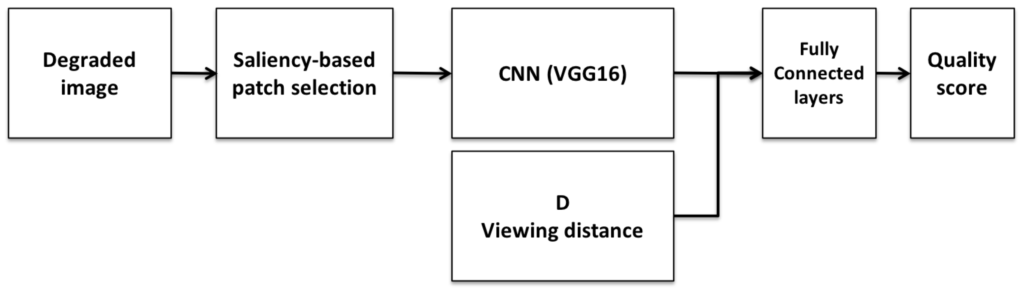
3. Proposed Method
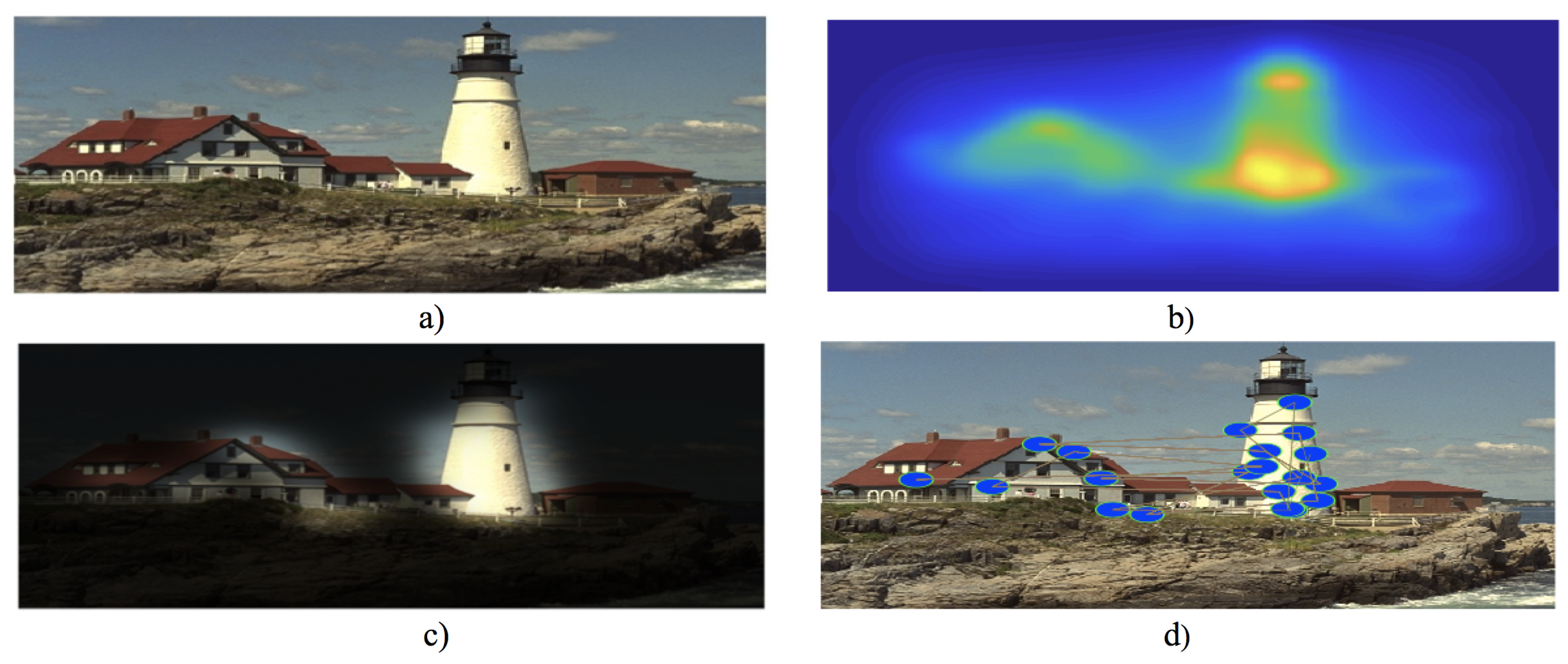
3.1. Saliency-Based Patch Selection
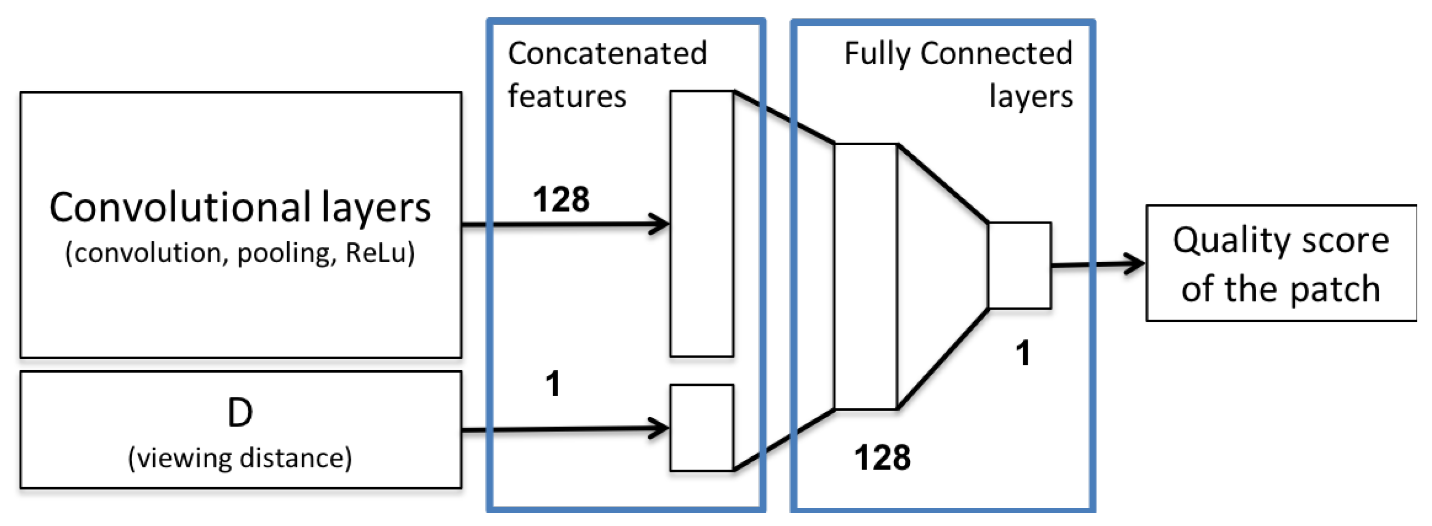
3.2. Cnn Model
3.3. Datasets
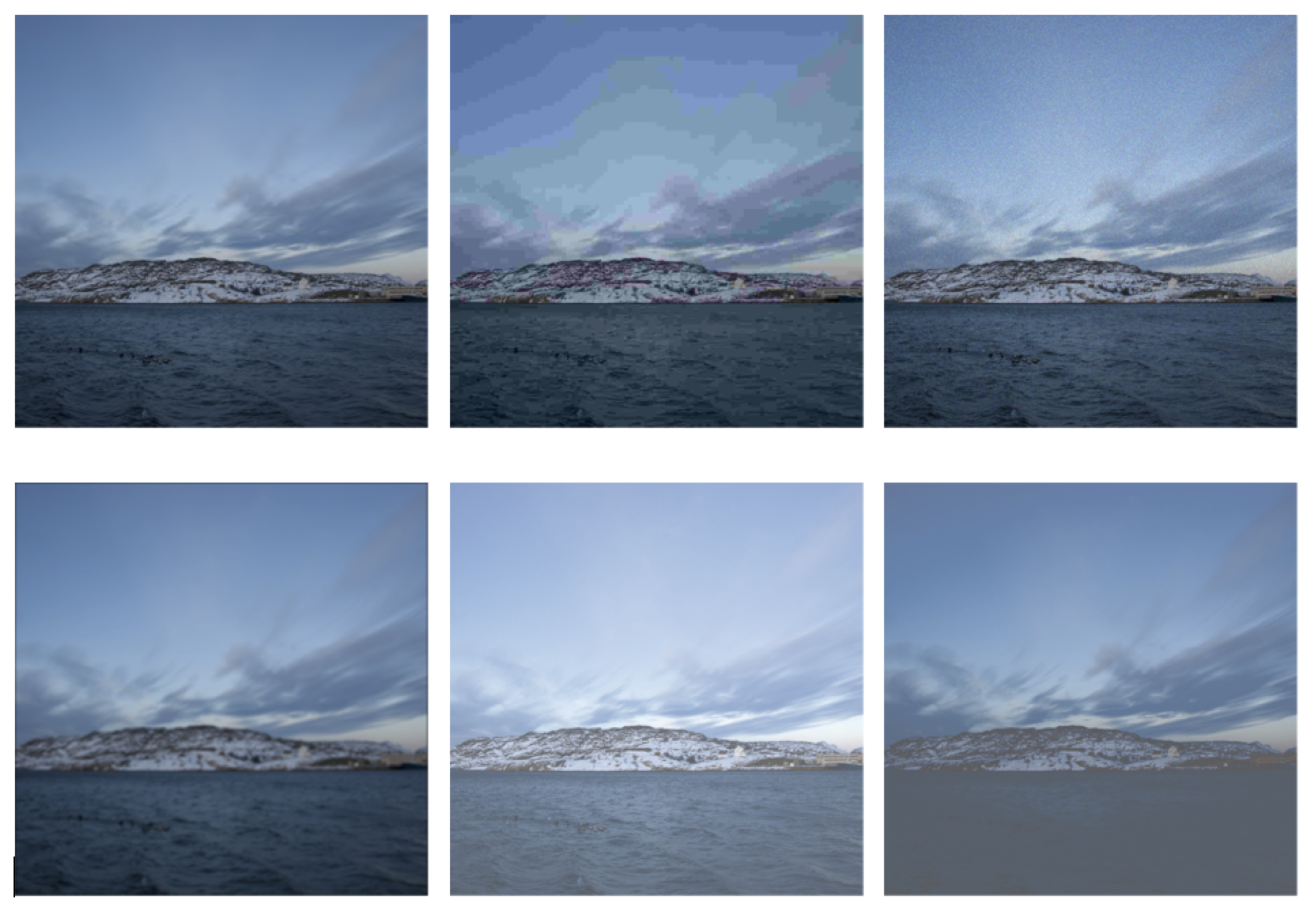
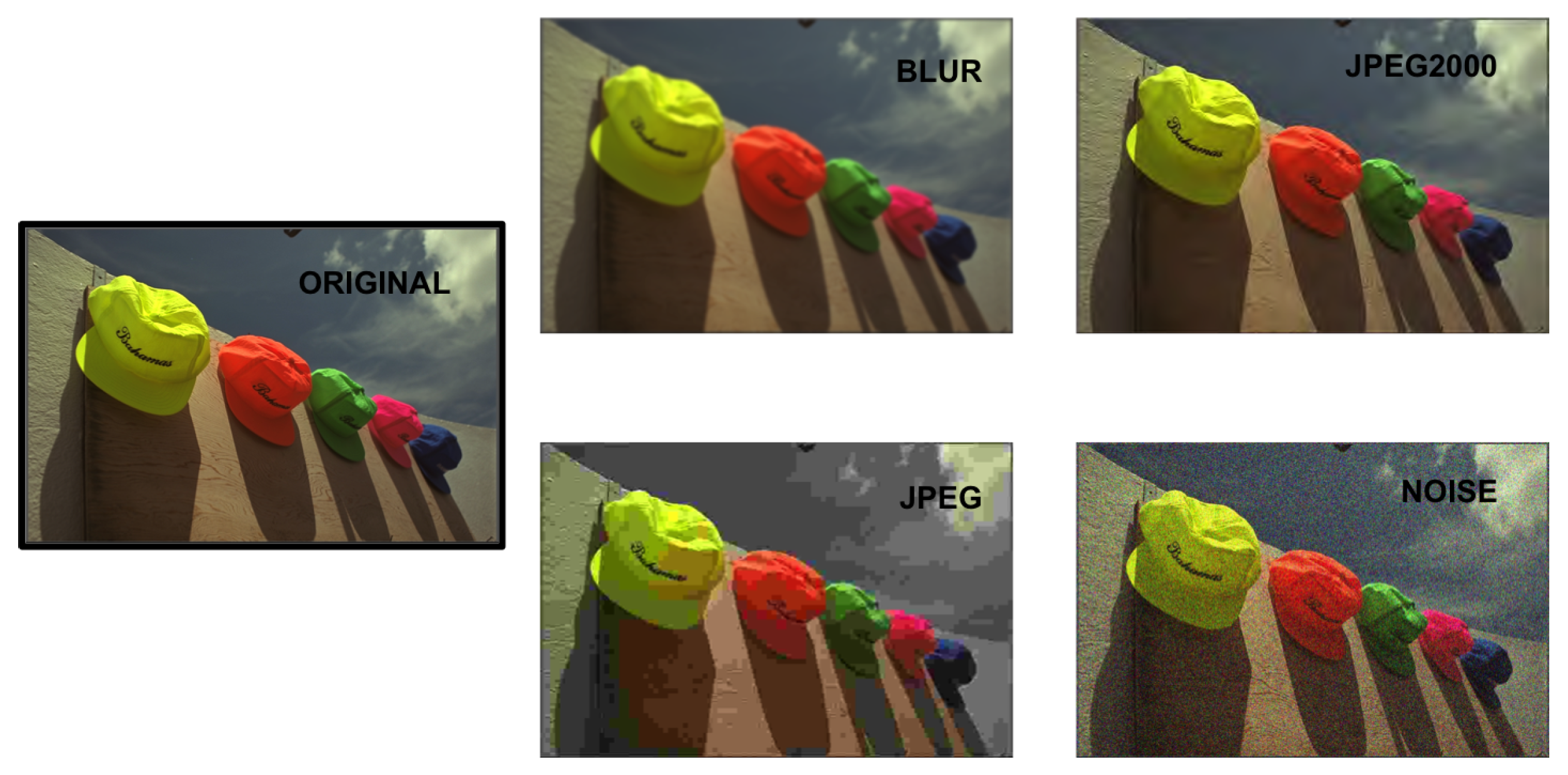
- CID:IQ (Colourlab Image Database: Image Quality) [52]: This dataset is one of the few publicly available datasets with subjective scores collected at different viewing distances. CID:IQ has 690 distorted images made from 23 original images with high-quality. Subjective scores were collected at two viewing distances (50 cm and 100 cm, which correspond respectively to 2.5 and 5 times the image height) for each distorted image. Distorted images were generated with six types of degradation at different five levels: JPEG2000 (JP2K), JPEG, Gaussian Blur (GB), Poisson noise (PN), gamut mapping (DeltaE) and SGCK gamut mapping (SGCK). An original image and five distorted images are presented in Figure 4.
- VDID2014 (Viewing Distance-changed Image Database) [53]: This dataset has 160 distorted images made from 8 high-quality images. For each distorted image, subjective scores were collected at two different distances (4 and 6 times the image height). Distorted images were made using four types of degradation at five different levels: JPEG2000 (JP2K), JPEG, Gaussian Blur (GB) and White Noise (WN). An example of distorted images is shown in Figure 5.
3.4. Evaluation Criteria
4. Experimental Results
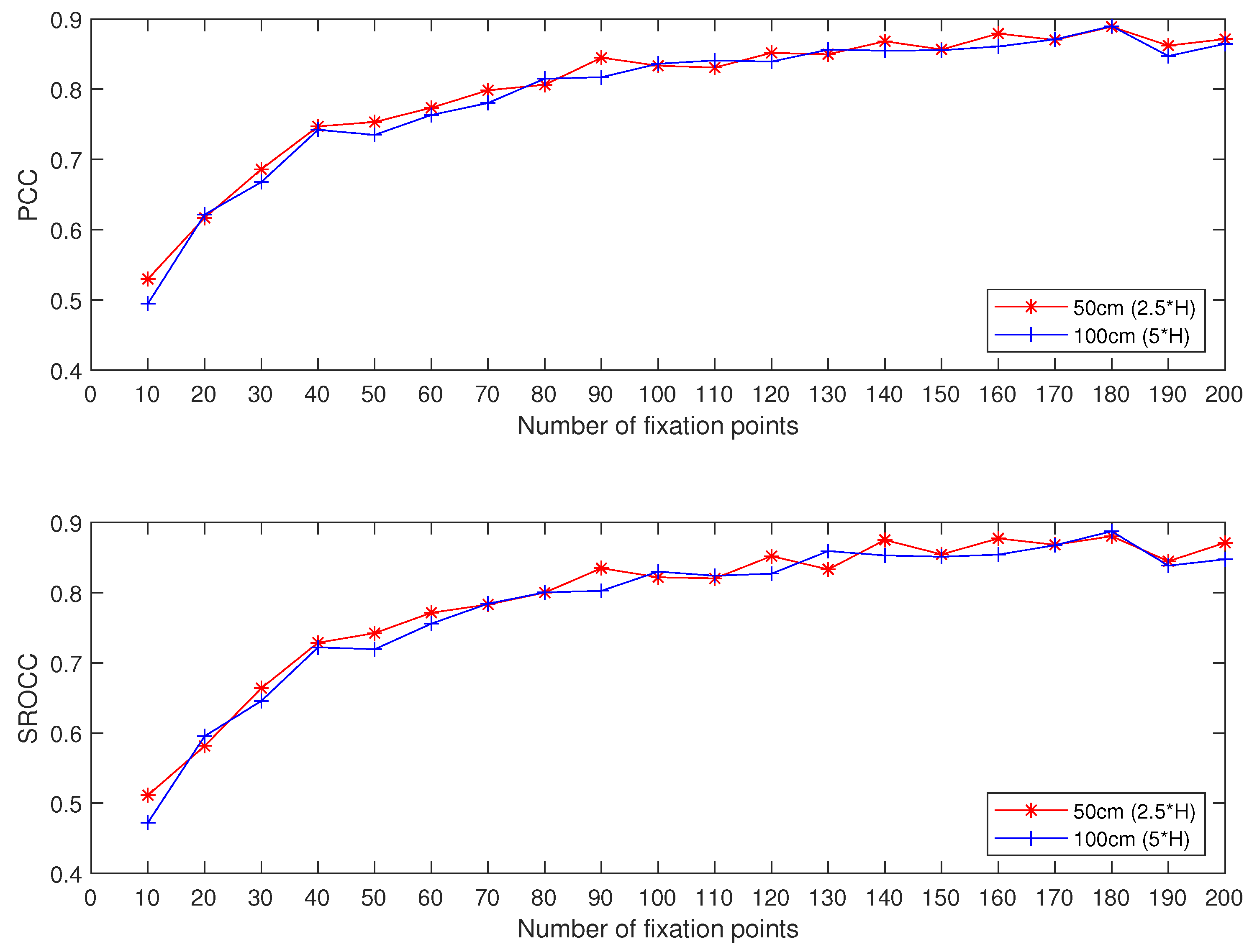
4.1. Impact of the Number of Fixation Points
4.2. Individual Evaluation
4.2.1. CID:IQ
4.2.2. Vdid2014
4.2.3. Computation Time
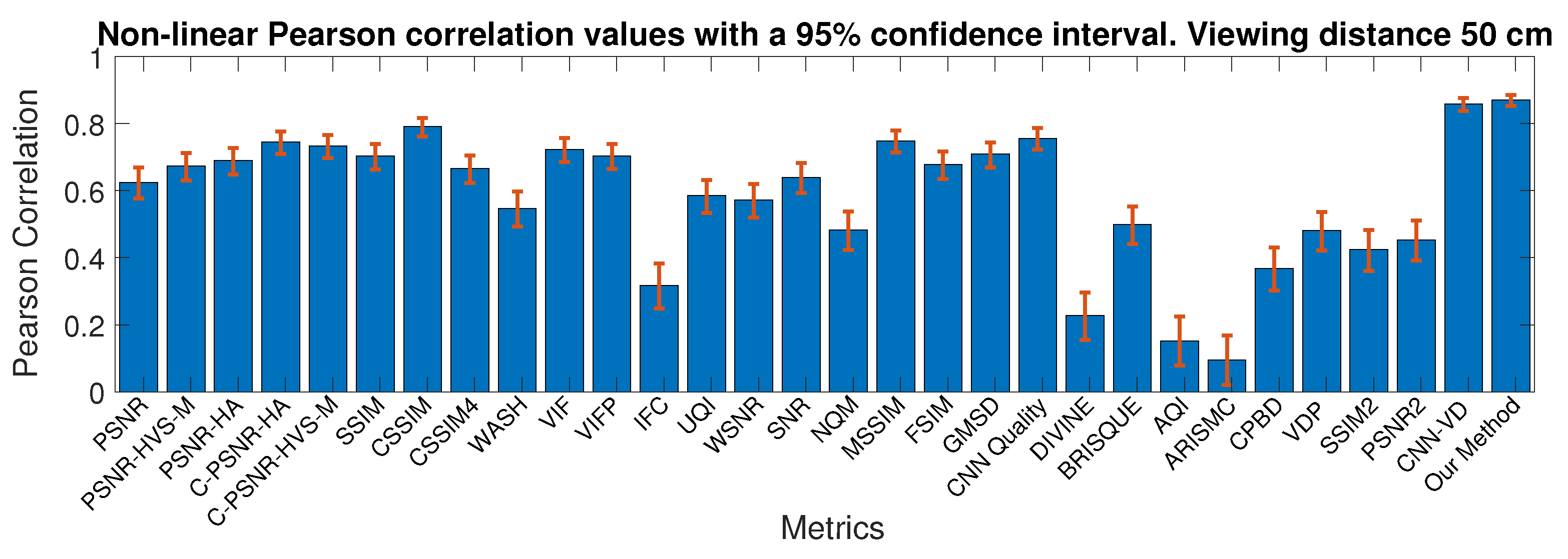
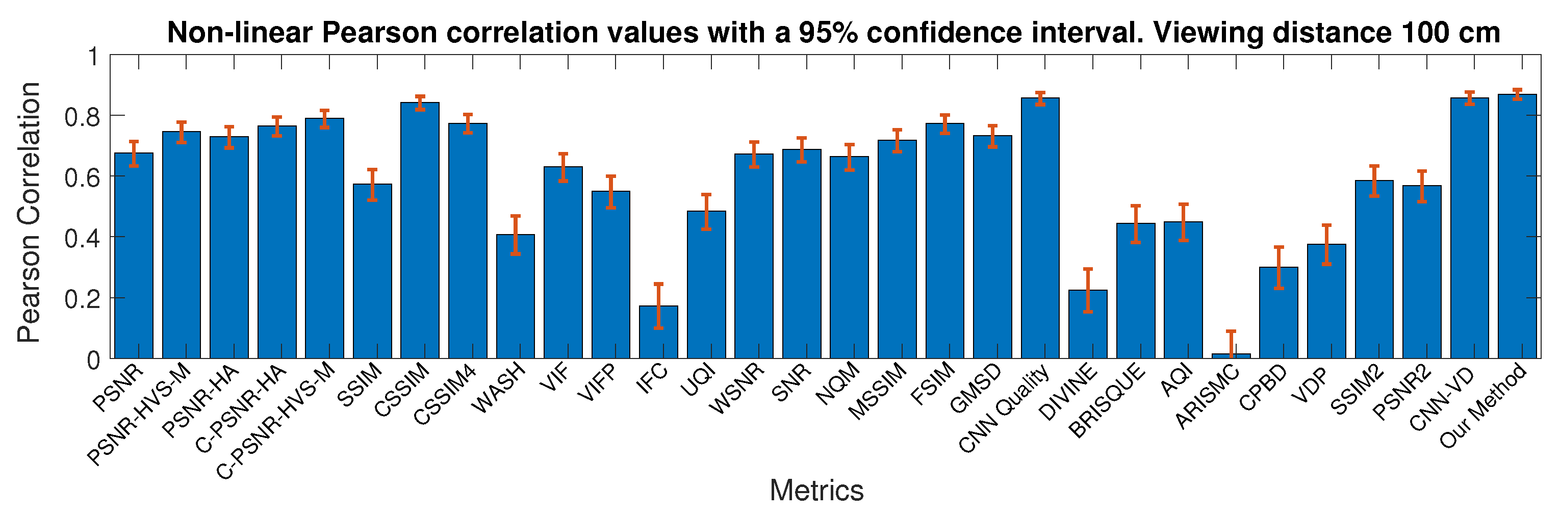
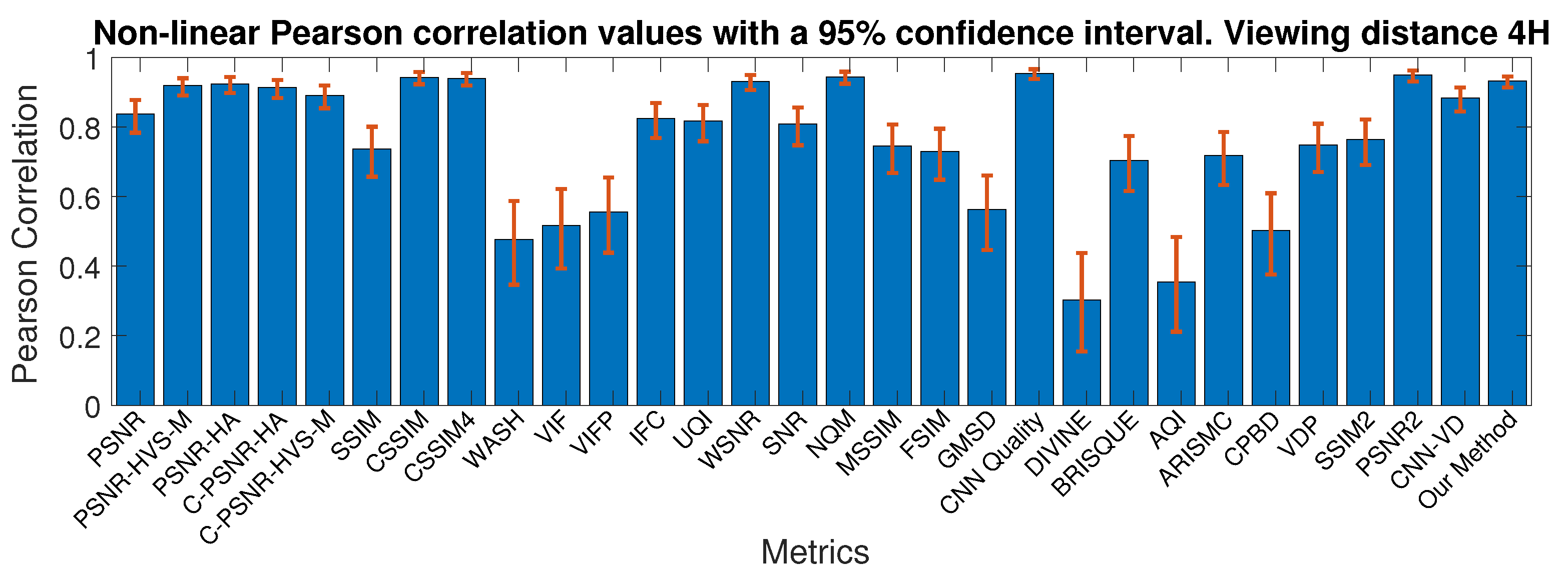
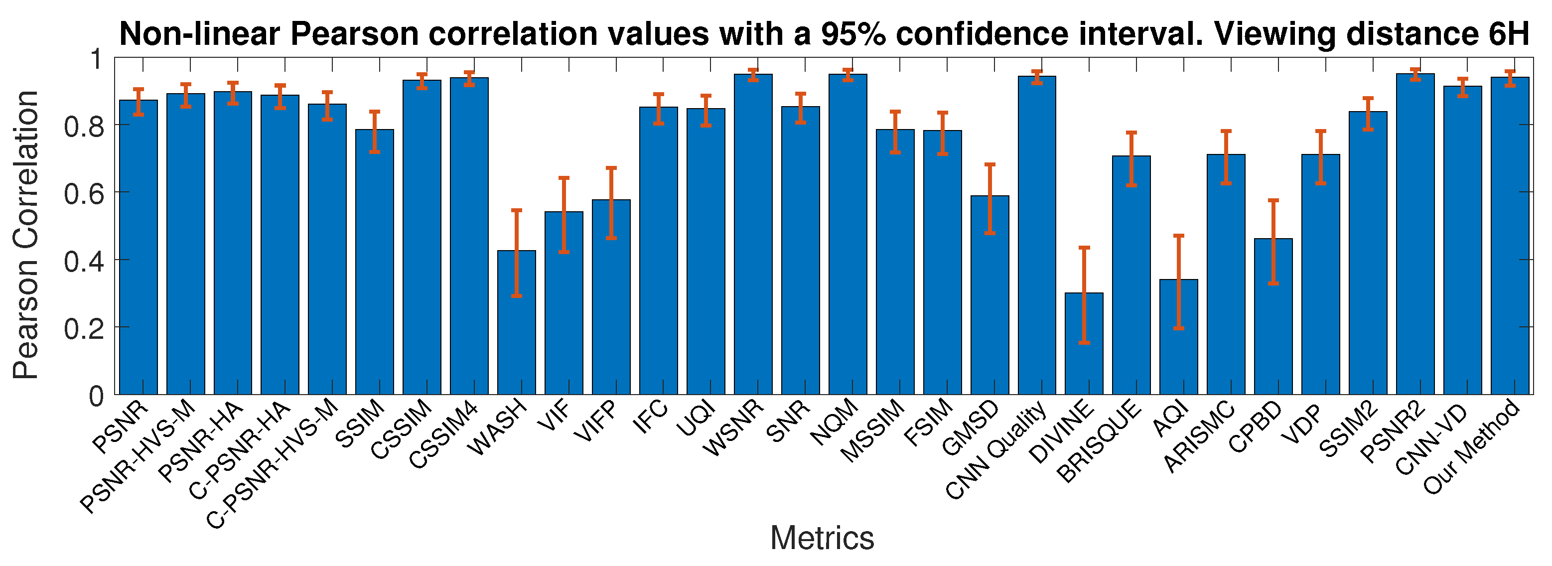
4.2.4. Comparison with the State-Of-The-Art
4.3. Cross Dataset Evaluation
5. Conclusions
Author Contributions
Funding
Conflicts of Interest
References
- Pedersen, M.; Hardeberg, J.Y. Full-reference image quality metrics: Classification and evaluation. Found. Trends® Comput. Graph. Vis. 2012, 7, 1–80. [Google Scholar]
- Lin, W.; Kuo, C.C.J. Perceptual visual quality metrics: A survey. J. Vis. Commun. Image Represent. 2011, 22, 297–312. [Google Scholar] [CrossRef]
- Engelke, U.; Zepernick, H.J. Perceptual-based quality metrics for image and video services: A survey. In Proceedings of the 2007 Next Generation Internet Networks, Trondheim, Norway, 21–23 May 2007; pp. 190–197. [Google Scholar]
- Thung, K.H.; Raveendran, P. A survey of image quality measures. In Proceedings of the 2009 International Conference for Technical Postgraduates (TECHPOS), Kuala Lumpur, Malaysia, 14–15 December 2009; pp. 1–4. [Google Scholar]
- Eskicioglu, A.M.; Fisher, P.S. Image quality measures and their performance. IEEE Trans. Commun. 1995, 43, 2959–2965. [Google Scholar] [CrossRef]
- Ahumada, A.J. Computational image quality metrics: A review. SID Dig. 1993, 24, 305–308. [Google Scholar]
- Pedersen, M. Evaluation of 60 full-reference image quality metrics on the CID:IQ. In Proceedings of the IEEE International Conference on Image Processing, Quebec City, QC, Canada, 27–30 September 2015; pp. 1588–1592. [Google Scholar]
- Chetouani, A. Full Reference Image Quality Assessment: Limitation. In Proceedings of the 2014 22nd International Conference on Pattern Recognition, Stockholm, Sweden, 24–28 August 2014; pp. 833–837. [Google Scholar]
- Avcibas, I.; Sankur, B.; Sayood, K. Statistical evaluation of image quality measures. J. Electron. Imaging 2002, 11, 206–224. [Google Scholar]
- Ponomarenko, N.; Lukin, V.; Zelensky, A.; Egiazarian, K.; Carli, M.; Battisti, F. TID2008-a database for evaluation of full-reference visual quality assessment metrics. Adv. Mod. Radioelectron. 2009, 10, 30–45. [Google Scholar]
- Zhang, L.; Zhang, L.; Mou, X.; Zhang, D. A comprehensive evaluation of full reference image quality assessment algorithms. In Proceedings of the IEEE International Conference on Image Processing, Orlando, FL, USA, 30 September–3 October 2012; pp. 1477–1480. [Google Scholar] [CrossRef]
- Lahoulou, A.; Bouridane, A.; Viennet, E.; Haddadi, M. Full-reference image quality metrics performance evaluation over image quality databases. Arab. J. Sci. Eng. 2013, 38, 2327–2356. [Google Scholar] [CrossRef]
- Wang, Z. Objective Image Quality Assessment: Facing The Real-World Challenges. Electron. Imaging 2016, 2016, 1–6. [Google Scholar] [CrossRef][Green Version]
- Chandler, D.M. Seven challenges in image quality assessment: Past, present, and future research. ISRN Signal Process. 2013, 2013. [Google Scholar] [CrossRef]
- Amirshahi, S.A.; Pedersen, M. Future Directions in Image Quality. In Color and Imaging Conference; Society for Imaging Science and Technology: Paris, France, 2019; Volume 2019, pp. 399–403. [Google Scholar]
- Wang, Z.; Bovik, A.C.; Lu, L. Why is image quality assessment so difficult? In Proceedings of the 2002 IEEE International Conference on Acoustics, Speech, and Signal Processing, Orlando, FL, USA, 13–17 May 2002; Volume 4, p. IV-3313. [Google Scholar]
- Wang, Z.; Bovik, A.C. Modern image quality assessment. Synth. Lect. Image Video Multimed. Process. 2006, 2, 1–156. [Google Scholar] [CrossRef]
- Wang, Z.; Bovik, A.C.; Sheikh, H.R.; Simoncelli, E.P. Image quality assessment: From error visibility to structural similarity. IEEE Trans. Image Process. 2004, 13, 600–612. [Google Scholar] [CrossRef]
- Zhang, X.; Wandell, B. A spatial extension of CIELAB for digital color-image reproduction. J. Soc. Inf. Disp. 1997, 5, 61–63. [Google Scholar] [CrossRef]
- Pedersen, M. An image difference metric based on simulation of image detail visibility and total variation. In Color and Imaging Conference. Society for Imaging Science and Technology; Society for Imaging Science and Technology: Boston, MA, USA, 2014; Volume 2014, pp. 37–42. [Google Scholar]
- Ponomarenko, N.; Silvestri, F.; Egiazarian, K.; Carli, M.; Astola, J.; Lukin, V. On between-coefficient contrast masking of DCT basis functions. In Proceedings of the Third International Workshop on Video Processing and Quality Metrics; Scottsdale, AZ, USA, 2007; Volume 4. [Google Scholar]
- Ajagamelle, S.A.; Pedersen, M.; Simone, G. Analysis of the difference of gaussians model in image difference metrics. In Conference on Colour in Graphics, Imaging, and Vision; Society for Imaging Science and Technology: Joensuu, Finland, 2010; Volume 2010, pp. 489–496. [Google Scholar]
- Charrier, C.; Lézoray, O.; Lebrun, G. Machine learning to design full-reference image quality assessment algorithm. Signal Process. Image Commun. 2012, 27, 209–219. [Google Scholar] [CrossRef]
- Pedersen, M.; Hardeberg, J.Y. A new spatial filtering based image difference metric based on hue angle weighting. J. Imaging Sci. Technol. 2012, 56, 50501-1. [Google Scholar] [CrossRef]
- Fei, X.; Xiao, L.; Sun, Y.; Wei, Z. Perceptual image quality assessment based on structural similarity and visual masking. Signal Process. Image Commun. 2012, 27, 772–783. [Google Scholar] [CrossRef]
- Pedersen, M.; Farup, I. Simulation of image detail visibility using contrast sensitivity functions and wavelets. In Color and Imaging Conference; Society for Imaging Science and Technology: Los Angeles, CA, USA, 2012; Volume 2012, pp. 70–75. [Google Scholar]
- Bai, J.; Nakaguchi, T.; Tsumura, N.; Miyake, Y. Evaluation of Image Corrected by Retinex Method Based on S-CIELAB and Gazing Information. IEICE Trans. 2006, 89-A, 2955–2961. [Google Scholar] [CrossRef]
- Pedersen, M.; Hardeberg, J.Y.; Nussbaum, P. Using gaze information to improve image difference metrics. In Human Vision and Electronic Imaging XIII; International Society for Optics and Photonics: San Jose, CA, USA, 2008; Volume 6806, p. 680611. [Google Scholar]
- Pedersen, M.; Zheng, Y.; Hardeberg, J.Y. Evaluation of image quality metrics for color prints. In Scandinavian Conference on Image Analysis; Springer: Berlin/Heidelberg, Germany, 2011; pp. 317–326. [Google Scholar]
- Falkenstern, K.; Bonnier, N.; Brettel, H.; Pedersen, M.; Viénot, F. Using image quality metrics to evaluate an icc printer profile. In Color and Imaging Conference; Society for Imaging Science and Technology: San Antonio, TX, USA, 2010; Volume 2010, pp. 244–249. [Google Scholar]
- Gong, M.; Pedersen, M. Spatial pooling for measuring color printing quality attributes. J. Vis. Commun. Image Represent. 2012, 23, 685–696. [Google Scholar] [CrossRef]
- Zhao, P.; Cheng, Y.; Pedersen, M. Objective assessment of perceived sharpness of projection displays with a calibrated camera. In Proceedings of the 2015 Colour and Visual Computing Symposium (CVCS), Gjovik, Norway, 25–26 August 2015; pp. 1–6. [Google Scholar]
- Charrier, C.; Knoblauch, K.; Maloney, L.T.; Bovik, A.C. Calibrating MS-SSIM for compression distortions using MLDS. In Proceedings of the 2011 18th IEEE International Conference on Image Processing, Brussels, Belgium, 11–14 September 2011; pp. 3317–3320. [Google Scholar]
- Brooks, A.C.; Pappas, T.N. Using structural similarity quality metrics to evaluate image compression techniques. In Proceedings of the 2007 IEEE International Conference on Acoustics, Speech and Signal Processing-ICASSP’07, Honolulu, HI, USA, 15–20 April 2007; Volume 1, p. I-873. [Google Scholar]
- Seybold, T.; Keimel, C.; Knopp, M.; Stechele, W. Towards an evaluation of denoising algorithms with respect to realistic camera noise. In Proceedings of the 2013 IEEE International Symposium on Multimedia, Anaheim, CA, USA, 9–11 December 2013; pp. 203–210. [Google Scholar]
- Amirshahi, S.A.; Kadyrova, A.; Pedersen, M. How do image quality metrics perform on contrast enhanced images? In Proceedings of the 2019 8th European Workshop on Visual Information Processing (EUVIP), Roma, Italy, 28–31 October 2019; pp. 232–237. [Google Scholar]
- Cao, G.; Pedersen, M.; Barańczuk, Z. Saliency models as gamut-mapping artifact detectors. In Conference on Colour in Graphics, Imaging, and Vision; Society for Imaging Science and Technology: Joensuu, Finland, 2010; Volume 2010, pp. 437–443. [Google Scholar]
- Hardeberg, J.Y.; Bando, E.; Pedersen, M. Evaluating colour image difference metrics for gamut-mapped images. Coloration Technol. 2008, 124, 243–253. [Google Scholar] [CrossRef]
- Pedersen, M.; Cherepkova, O.; Mohammed, A. Image Quality Metrics for the Evaluation and Optimization of Capsule Video Endoscopy Enhancement Techniques. J. Imaging Sci. Technol. 2017, 61, 40402-1. [Google Scholar] [CrossRef]
- Völgyes, D.; Martinsen, A.; Stray-Pedersen, A.; Waaler, D.; Pedersen, M. A Weighted Histogram-Based Tone Mapping Algorithm for CT Images. Algorithms 2018, 11, 111. [Google Scholar] [CrossRef]
- Yao, Z.; Le Bars, J.; Charrier, C.; Rosenberger, C. Fingerprint Quality Assessment Combining Blind Image Quality, Texture and Minutiae Features. In Proceedings of the 1st International Conference on Information Systems Security and Privacy; ESEO: Angers, Loire Valley, France, 2015; pp. 336–343. [Google Scholar]
- Liu, X.; Pedersen, M.; Charrier, C.; Bours, P. Performance evaluation of no-reference image quality metrics for face biometric images. J. Electron. Imaging 2018, 27, 023001. [Google Scholar] [CrossRef]
- Jenadeleh, M.; Pedersen, M.; Saupe, D. Blind Quality Assessment of Iris Images Acquired in Visible Light for Biometric Recognition. Sensors 2020, 20, 1308. [Google Scholar] [CrossRef] [PubMed]
- Bianco, S.; Celona, L.; Napoletano, P.; Schettini, R. On the Use of Deep Learning for Blind Image Quality Assessment. Signal Image Video Process. 2018, 12, 355–362. [Google Scholar] [CrossRef]
- Kang, L.; Ye, P.; Li, Y.; Doermann, D. Convolutional Neural Networks for No-Reference Image Quality Assessment. In Proceedings of the IEEE Conference on Computer Vision and Pattern Recognition, Columbus, OH, USA, 23–28 June 2014; pp. 1733–1740. [Google Scholar]
- Li, Y.; Po, L.M.; Xu, X.; Feng, L.; Yuan, F.; Cheung, C.H.; Cheung, K.W. No-reference image quality assessment with shearlet transform and deep neural networks. Neurocomputing 2015, 154, 94–109. [Google Scholar] [CrossRef]
- Kim, J.; Lee, S. Fully deep blind image quality predictor. IEEE J. Sel. Top. Signal Process. 2017, 11, 206–220. [Google Scholar] [CrossRef]
- Lv, Y.; Jiang, G.; Yu, M.; Xu, H.; Shao, F.; Liu, S. Difference of Gaussian statistical features based blind image quality assessment: A deep learning approach. In Proceedings of the IEEE International Conference on Image Processing, Quebec City, QC, Canada, 27–30 September 2015; pp. 2344–2348. [Google Scholar]
- Gao, F.; Wang, Y.; Li, P.; Tan, M.; Yu, J.; Zhu, Y. DeepSim: Deep similarity for image quality assessment. Neurocomputing 2017, 257, 104–114. [Google Scholar] [CrossRef]
- Hou, W.; Gao, X.; Tao, D.; Li, X. Blind image quality assessment via deep learning. IEEE Trans. Neural Netw. Learn. Syst. 2014, 26, 1275–1286. [Google Scholar]
- Amirshahi, S.A.; Pedersen, M.; Yu, S.X. Image quality assessment by comparing CNN features between images. J. Imaging Sci. Technol. 2016, 60, 60410-1. [Google Scholar] [CrossRef]
- Liu, X.; Pedersen, M.; Hardeberg, J. CID:IQ-A New Image Quality Database. In Image and Signal Processing; Springer: Berlin/Heidelberg, Germany, 2014; pp. 193–202. [Google Scholar]
- Gu, K.; Liu, M.; Zhai, G.; Yang, X.; Zhang, W. Quality assessment considering viewing distance and image resolution. IEEE Trans. Broadcasting 2015, 61, 520–531. [Google Scholar] [CrossRef]
- Chetouani, A.; Beghdadi, A.; Deriche, M.A. A hybrid system for distortion classification and image quality evaluation. Sig. Proc. Image Comm. 2012, 27, 948–960. [Google Scholar] [CrossRef]
- Sheikh, H. LIVE Image Quality Assessment Database Release 2. 2005. Available online: http://live.ece.utexas.edu/research/quality (accessed on 12 April 2021).
- Chetouani, A. Convolutional Neural Network and Saliency Selection for Blind Image Quality Assessment. In Proceedings of the IEEE International Conference on Image Processing, Athens, Greece, 7–10 October 2018; pp. 2835–2839. [Google Scholar]
- Larson, E.C.; Chandler, D.M. Most apparent distortion: Full-reference image quality assessment and the role of strategy. J. Electron. Imaging 2010, 19, 011006. [Google Scholar]
- Chetouani, A. Blind Utility and Quality Assessment Using a Convolutional Neural Network and a Patch Selection. In Proceedings of the 2019 IEEE International Conference on Image Processing (ICIP), Taipei, Taiwan, 22–25 September 2019; pp. 459–463. [Google Scholar]
- Rouse, D.M.; Hemami, S.S.; Pépion, R.; Le Callet, P. Estimating the usefulness of distorted natural images using an image contour degradation measure. JOSA A 2011, 28, 157–188. [Google Scholar] [CrossRef]
- Ninassi, A.; Le Callet, P.; Autrusseau, F. Subjective Quality Assessment-IVC Database. 2006. Available online: http://www.irccyn.ec-nantes.fr/ivcdb (accessed on 24 March 2018).
- Horita, Y.; Shibata, K.; Kawayoke, Y.; Sazzad, Z.P. MICT Image Quality Evaluation Database. 2011. Available online: http://mict.eng.u-toyama.ac.jp/mictdb.html (accessed on 27 July 2015).
- Jayaraman, D.; Mittal, A.; Moorthy, A.K.; Bovik, A.C. Objective quality assessment of multiply distorted images. In Proceedings of the 2012 Conference Record of the Forty Sixth Asilomar Conference on Signals, Systems and Computers (ASILOMAR), Pacific Grove, CA, USA, 4–7 November 2012; pp. 1693–1697. [Google Scholar]
- Jia, Y.; Shelhamer, E.; Donahue, J.; Karayev, S.; Long, J.; Girshick, R.; Guadarrama, S.; Darrell, T. Caffe: Convolutional architecture for fast feature embedding. In Proceedings of the 22nd ACM International Conference on Multimedia, Orlando, FL, USA, 3–7 November 2014; pp. 675–678. [Google Scholar]
- Ghadiyaram, D.; Bovik, A.C. Massive online crowdsourced study of subjective and objective picture quality. IEEE Trans. Image Process. 2015, 25, 372–387. [Google Scholar] [CrossRef] [PubMed]
- Ponomarenko, N.; Jin, L.; Ieremeiev, O.; Lukin, V.; Egiazarian, K.; Astola, J.; Vozel, B.; Chehdi, K.; Carli, M.; Battisti, F.; et al. Image database TID2013: Peculiarities, results and perspectives. Signal Process. Image Commun. 2015, 30, 57–77. [Google Scholar] [CrossRef]
- Li, J.; Zou, L.; Yan, J.; Deng, D.; Qu, T.; Xie, G. No-reference image quality assessment using Prewitt magnitude based on convolutional neural networks. Signal Image Video Process. 2016, 10, 609–616. [Google Scholar] [CrossRef]
- Simonyan, K.; Zisserman, A. Very deep convolutional networks for large-scale image recognition. arXiv 2014, arXiv:1409.1556. [Google Scholar]
- Fan, C.; Zhang, Y.; Feng, L.; Jiang, Q. No reference image quality assessment based on multi-expert convolutional neural networks. IEEE Access 2018, 6, 8934–8943. [Google Scholar] [CrossRef]
- Ravela, R.; Shirvaikar, M.; Grecos, C. No-reference image quality assessment based on deep convolutional neural networks. In Real-Time Image Processing and Deep Learning 2019; International Society for Optics and Photonics: Bellingham, WA, USA, 2019; Volume 10996, p. 1099604. [Google Scholar]
- Varga, D. Multi-Pooled Inception Features for No-Reference Image Quality Assessment. Appl. Sci. 2020, 10, 2186. [Google Scholar] [CrossRef]
- Ma, J.; Wu, J.; Li, L.; Dong, W.; Xie, X.; Shi, G.; Lin, W. Blind Image Quality Assessment With Active Inference. IEEE Trans. Image Process. 2021, 30, 3650–3663. [Google Scholar] [CrossRef]
- Krizhevsky, A.; Sutskever, I.; Hinton, G.E. Imagenet classification with deep convolutional neural networks. In Advances in Neural Information Processing Systems; Curran Associates, Inc.: Red Hook, NY, USA, 2012; pp. 1097–1105. [Google Scholar]
- Beghdadi, A.; Qureshi, M.A.; Sdiri, B.; Deriche, M.; Alaya-Cheikh, F. Ceed-A Database for Image Contrast Enhancement Evaluation. In Proceedings of the 2018 Colour and Visual Computing Symposium (CVCS), Gjovik, Norway, 19–20 September 2018; pp. 1–6. [Google Scholar]
- Amirshahi, S.; Pedersen, M.; Beghdadi, A. Reviving Traditional Image Quality Metrics Using CNNs. In Color and Imaging Conference; Society for Imaging Science and Technology: Paris, France, 2018; pp. 241–246. [Google Scholar]
- Le Meur, O.; Liu, Z. Saccadic model of eye movements for free-viewing condition. Vis. Res. 2015, 116, 152–164. [Google Scholar] [CrossRef] [PubMed]
- Bosse, S.; Maniry, D.; Müller, K.; Wiegand, T.; Samek, W. Deep Neural Networks for No-Reference and Full-Reference Image Quality Assessment. IEEE Trans. Image Process. 2018, 27, 206–219. [Google Scholar] [CrossRef]
- Vigier, T.; Da Silva, M.P.; Le Callet, P. Impact of visual angle on attention deployment and robustness of visual saliency models in videos: From SD to UHD. In Proceedings of the 2016 IEEE International Conference on Image Processing (ICIP), Phoenix, AZ, USA, 25–28 September 2016; pp. 689–693. [Google Scholar]
- Harel, J.; Koch, C.; Perona, P. Graph-based visual saliency. In Advances in Neural Information Processing Systems; MIT Press: Cambridge, MA, USA, 2007; pp. 545–552. [Google Scholar]
- Borji, A.; Tavakoli, H.R.; Sihite, D.N.; Itti, L. Analysis of scores, datasets, and models in visual saliency prediction. In Proceedings of the IEEE International Conference on Computer Vision, 2013, Sydney, NSW, Australia, 1–8 December 2013; pp. 921–928. [Google Scholar]
- Chetouani, A. A Blind Image Quality Metric using a Selection of Relevant Patches based on Convolutional Neural Network. In Proceedings of the European Signal Processing Conference, Rome, Italy, 3–7 September 2018; pp. 1452–1456. [Google Scholar]
- He, K.; Zhang, X.; Ren, S.; Sun, J. Deep residual learning for image recognition. arXiv 2015, arXiv:1512.03385. [Google Scholar]
- Chetouani, A.; Treuillet, S.; Exbrayat, M.; Jesset, S. Classification of engraved pottery sherds mixing deep-learning features by compact bilinear pooling. Pattern Recognit. Lett. 2020, 131, 1–7. [Google Scholar] [CrossRef]
- Elloumi, W.; Chetouani, A.; Charrada, T.; Fourati, E. Anti-Spoofing in Face Recognition: Deep Learning and Image Quality Assessment-Based Approaches. In Deep Biometrics. Unsupervised and Semi-Supervised Learning; Jiang, R., Li, C.T., Crookes, D., Meng, W., Rosenberger, C., Eds.; Springer: Cham, Switzerland, 2020. [Google Scholar]
- Abouelaziz, I.; Chetouani, A.; El Hassouni, M.; Latecki, L.; Cherifi, H. No-reference mesh visual quality assessment via ensemble of convolutional neural networks and compact multi-linear pooling. Pattern Recognit. 2020, 100, 107174. [Google Scholar] [CrossRef]
- Chetouani, A.; Li, L. On the use of a scanpath predictor and convolutional neural network for blind image quality assessment. Signal Process. Image Commun. 2020, 89, 115963. [Google Scholar] [CrossRef]
- Chetouani, A. Image Quality Assessment Without Reference By Mixing Deep Learning-Based Features. In Proceedings of the IEEE International Conference on Multimedia and Expo, ICME 2020, London, UK, 6–10 July 2020; pp. 1–6. [Google Scholar] [CrossRef]
- Furmanski, C.S.; Engel, S.A. An oblique effect in human primary visual cortex. Nat. Neurosci. 2000, 3, 535–536. [Google Scholar] [CrossRef] [PubMed]
- Kim, H.; Lee, S. Transition of Visual Attention Assessment in Stereoscopic Images with Evaluation of Subjective Visual Quality and Discomfort. IEEE Trans. Multimed. 2015, 17, 2198–2209. [Google Scholar] [CrossRef]
- Ponomarenko, N.; Ieremeiev, O.; Lukin, V.; Egiazarian, K.; Carli, M. Modified image visual quality metrics for contrast change and mean shift accounting. In Proceedings of the 2011 11th International Conference The Experience of Designing and Application of CAD Systems in Microelectronics (CADSM), Polyana, Ukraine, 23–25 February 2011; pp. 305–311. [Google Scholar]
- Ponomarenko, M.; Egiazarian, K.; Lukin, V.; Abramova, V. Structural similarity index with predictability of image blocks. In Proceedings of the 2018 IEEE 17th International Conference on Mathematical Methods in Electromagnetic Theory (MMET), Kyiv, UKraine, 2–5 July 2018; pp. 115–118. [Google Scholar]
- Reenu, M.; David, D.; Raj, S.A.; Nair, M.S. Wavelet based sharp features (WASH): An image quality assessment metric based on HVS. In Proceedings of the 2013 2nd International Conference on Advanced Computing, Networking and Security, Wavelet Based Sharp Features (WASH): An Image Quality Assessment Metric Based on HVS, Mangalore, India, 15–17 December 2013; pp. 79–83. [Google Scholar]
- Sheikh, H.R.; Bovik, A.C. Image information and visual quality. IEEE Trans. Image Process. 2006, 15, 430–444. [Google Scholar] [CrossRef] [PubMed]
- Sheikh, H.R.; Bovik, A.C.; de Veciana, G. An information fidelity criterion for image quality assessment using natural scene statistics. IEEE Trans. Image Process. 2005, 14, 2117–2128. [Google Scholar] [CrossRef] [PubMed]
- Wang, Z.; Bovik, A.C. A universal image quality index. IEEE Signal Process. Lett. 2002, 9, 81–84. [Google Scholar] [CrossRef]
- Mitsa, T.; Varkur, K.L. Evaluation of contrast sensitivity functions for the formulation of quality measures incorporated in halftoning algorithms. In Proceedings of the 1993 IEEE International Conference on Acoustics, Speech, and Signal Processing, Minneapolis, MN, USA, 27–30 April 1993; Volume 5, pp. 301–304. [Google Scholar] [CrossRef]
- Damera-Venkata, N.; Kite, T.D.; Geisler, W.S.; Evans, B.L.; Bovik, A.C. Image quality assessment based on a degradation model. IEEE Trans. Image Process. 2000, 9, 636–650. [Google Scholar] [CrossRef]
- Wang, Z.; Simoncelli, E.P.; Bovik, A.C. Multiscale structural similarity for image quality assessment. In Proceedings of the The Thrity-Seventh Asilomar Conference on Signals, Systems Computers, Pacific Grove, CA, USA, 9–12 November 2003; Volume 2, pp. 1398–1402. [Google Scholar] [CrossRef]
- Zhang, L.; Zhang, L.; Mou, X.; Zhang, D. FSIM: A Feature Similarity Index for Image Quality Assessment. IEEE Trans. Image Process. 2011, 20, 2378–2386. [Google Scholar] [CrossRef]
- Xue, W.; Zhang, L.; Mou, X.; Bovik, A.C. Gradient Magnitude Similarity Deviation: A Highly Efficient Perceptual Image Quality Index. IEEE Trans. Image Process. 2014, 23, 684–695. [Google Scholar] [CrossRef]
- Anish Mittal, A.K.M.; Bovik, A.C. No-reference image quality assessment in the spatial domain. IEEE Trans. Image Process. 2012, 21, 4695–4708. [Google Scholar] [CrossRef] [PubMed]
- Moorthy, A.K.; Bovik, A.C. Blind image quality assessment: From natural scene statistics to perceptual quality. IEEE Trans. Image Process. 2011, 20, 3350–3364. [Google Scholar] [CrossRef]
- Gabarda, S.; Cristóbal, G. Blind image quality assessment through anisotropy. JOSA A 2007, 24, B42–B51. [Google Scholar] [CrossRef] [PubMed]
- Gu, K.; Zhai, G.; Lin, W.; Yang, X.; Zhang, W. No-reference image sharpness assessment in autoregressive parameter space. IEEE Trans. Image Process. 2015, 24, 3218–3231. [Google Scholar] [PubMed]
- Gu, K.; Zhai, G.; Lin, W.; Yang, X.; Zhang, W. Learning a blind quality evaluation engine of screen content images. Neurocomputing 2016, 196, 140–149. [Google Scholar] [CrossRef]
- Narvekar, N.D.; Karam, L.J. A no-reference perceptual image sharpness metric based on a cumulative probability of blur detection. In Proceedings of the 2009 International Workshop on Quality of Multimedia Experience, San Diego, CA, USA, 29–31 July 2009; pp. 87–91. [Google Scholar]
- Daly, S.J. Visible differences predictor: An algorithm for the assessment of image fidelity. In Proceedings of the SPIE 1666, Human Vision, Visual Processing, and Digital Display III; International Society for Optics and Photonics’: San Jose, CA, USA, 1992. [Google Scholar]
- Wang, Z.; Bovik, A.C. Embedded foveation image coding. IEEE Trans. Image Process. 2001, 10, 1397–1410. [Google Scholar] [CrossRef]


| Configuration | |
|---|---|
| Computer Model | DELL Precision 5820 |
| CPU | Intel Xeon W-2125 CPU 4.00 GHz (8 cores) |
| Memory | 64 GB |
| GPU | NVIDIA Quadro P5000 |
| 50 cm (2.5*H) | 100 cm (5*H) | ALL | ||||
|---|---|---|---|---|---|---|
| Selection | PCC | SROCC | PCC | SROCC | PCC | SROCC |
| Without integration of the viewing distance (baseline model) | ||||||
| Random | 0.670 | 0.667 | 0.637 | 0.621 | 0.641 | 0.629 |
| No | 0.725 | 0.736 | 0.664 | 0.659 | 0.681 | 0.682 |
| Saliency | 0.712 | 0.718 | 0.705 | 0.704 | 0.695 | 0.695 |
| With integration of the viewing distance (proposed model) | ||||||
| Random | 0.757 | 0.750 | 0.764 | 0.718 | 0.750 | 0.729 |
| No | 0.819 | 0.815 | 0.819 | 0.775 | 0.813 | 0.797 |
| Saliency | 0.870 | 0.867 | 0.870 | 0.846 | 0.876 | 0.865 |
| 50 cm (2.5*H) | 100 cm (5*H) | |||
|---|---|---|---|---|
| PCC | SROCC | PCC | SROCC | |
| CNN-VD (NR) | 0.858 | 0.855 | 0.858 | 0.826 |
| Our method (NR) | 0.870 | 0.867 | 0.870 | 0.846 |
| 50 cm (2.5*H) | |||
| Distortion type | Our method | MSSIM | CNN Quality |
| JP2K | 0.819 | 0.851 | 0.826 |
| JPEG | 0.812 | 0.736 | 0.801 |
| PN | 0.836 | 0.811 | 0.792 |
| GB | 0.870 | 0.576 | 0.882 |
| SGCK | 0.913 | 0.736 | 0.814 |
| DeltaE | 0.919 | 0.792 | 0.837 |
| 100 cm (5*H) | |||
| Distortion type | Our method | MSSIM | CNN Quality |
| JP2K | 0.735 | 0.825 | 0.804 |
| JPEG | 0.820 | 0.700 | 0.811 |
| PN | 0.793 | 0.838 | 0.771 |
| GB | 0.884 | 0.598 | 0.893 |
| SGCK | 0.938 | 0.725 | 0.805 |
| DeltaE | 0.923 | 0.780 | 0.862 |
| 4*H | 6*H | |||
|---|---|---|---|---|
| PCC | SROCC | PCC | SROCC | |
| CNN-VD (NR) | 0.884 | 0.871 | 0.914 | 0.898 |
| Our method (NR) | 0.932 | 0.907 | 0.940 | 0.922 |
| 4*H | |||
|---|---|---|---|
| Distortion Type | Our Method | MSSIM | CNN Quality |
| JP2K | 0.925 | 0.827 | 0.874 |
| JPEG | 0.969 | 0.876 | 0.874 |
| WN | 0.903 | 0.912 | 0.871 |
| GB | 0.913 | 0.773 | 0.901 |
| 6*H | |||
| Distortion Type | Our Method | MSSIM | CNN Quality |
| JP2K | 0.951 | 0.8461 | 0.896 |
| JPEG | 0.973 | 0.846 | 0.886 |
| WN | 0.930 | 0.895 | 0.895 |
| GB | 0.921 | 0.796 | 0.933 |
| Database | All Patches | Saliency-Based |
|---|---|---|
| Patch Selection | ||
| CID:IQ | 625 (≊75 ms) | 180 (≊21.6 ms) |
| VDID | 310 (≊37.2 ms) | 180 (≊26.6 ms) |
| CID:IQ | VDID2014 | |||||||
|---|---|---|---|---|---|---|---|---|
| 50 cm (2.5*H) | 100 cm (5*H) | 4*H | 6*H | |||||
| Metric | PCC | SROCC | PCC | SROCC | PCC | SROCC | PCC | SROCC |
| Full-Reference | ||||||||
| PSNR | 0.625 | 0.625 | 0.676 | 0.670 | 0.837 | 0.884 | 0.873 | 0.895 |
| PSNR-HVS-M | 0.673 | 0.664 | 0.746 | 0.739 | 0.919 | 0.945 | 0.891 | 0.930 |
| PSNR-HA | 0.690 | 0.687 | 0.730 | 0.729 | 0.924 | 0.940 | 0.897 | 0.933 |
| C-PSNR-HA | 0.745 | 0.743 | 0.765 | 0.769 | 0.913 | 0.943 | 0.887 | 0.931 |
| C-PSNR-HVS-M | 0.734 | 0.728 | 0.790 | 0.788 | 0.891 | 0.943 | 0.861 | 0.926 |
| SSIM | 0.703 | 0.756 | 0.573 | 0.633 | 0.737 | 0.927 | 0.786 | 0.934 |
| CSSIM | 0.791 | 0.792 | 0.842 | 0.828 | 0.943 | 0.945 | 0.932 | 0.929 |
| CSSIM4 | 0.666 | 0.636 | 0.774 | 0.753 | 0.940 | 0.934 | 0.939 | 0.921 |
| WASH | 0.547 | 0.524 | 0.408 | 0.404 | 0.476 | 0.476 | 0.427 | 0.432 |
| VIF | 0.723 | 0.720 | 0.631 | 0.626 | 0.517 | 0.694 | 0.541 | 0.700 |
| VIFP | 0.704 | 0.703 | 0.550 | 0.547 | 0.556 | 0.648 | 0.577 | 0.656 |
| IFC | 0.317 | 0.493 | 0.173 | 0.343 | 0.825 | 0.870 | 0.852 | 0.900 |
| UQI | 0.585 | 0.594 | 0.484 | 0.474 | 0.818 | 0.845 | 0.847 | 0.855 |
| WSNR | 0.572 | 0.560 | 0.673 | 0.654 | 0.931 | 0.937 | 0.949 | 0.952 |
| SNR | 0.640 | 0.636 | 0.688 | 0.671 | 0.809 | 0.853 | 0.854 | 0.871 |
| NQM | 0.483 | 0.469 | 0.664 | 0.632 | 0.944 | 0.928 | 0.949 | 0.936 |
| MSSIM | 0.748 | 0.827 | 0.718 | 0.789 | 0.746 | 0.930 | 0.785 | 0.936 |
| FSIM | 0.678 | 0.744 | 0.773 | 0.816 | 0.730 | 0.906 | 0.782 | 0.935 |
| GMSD | 0.709 | 0.743 | 0.733 | 0.767 | 0.563 | 0.902 | 0.589 | 0.905 |
| CNN Quality | 0.756 | 0.753 | 0.857 | 0.831 | 0.954 | 0.958 | 0.943 | 0.947 |
| No-Reference | ||||||||
| DIVINE | 0.227 | 0.259 | 0.225 | 0.247 | 0.303 | 0.274 | 0.301 | 0.266 |
| BRISQUE | 0.499 | 0.520 | 0.444 | 0.491 | 0.704 | 0.708 | 0.707 | 0.709 |
| AQI | 0.152 | 0.236 | 0.450 | 0.311 | 0.355 | 0.242 | 0.341 | 0.263 |
| ARISMC | 0.095 | 0.133 | 0.015 | 0.114 | 0.718 | 0.730 | 0.712 | 0.734 |
| CPBD | 0.368 | 0.299 | 0.300 | 0.245 | 0.502 | 0.504 | 0.461 | 0.486 |
| Distance-based | ||||||||
| VDP (FR) | 0.481 | 0.476 | 0.376 | 0.397 | 0.748 | 0.829 | 0.712 | 0.748 |
| SSIM2 (FR) | 0.424 | 0.549 | 0.586 | 0.682 | 0.764 | 0.942 | 0.838 | 0.959 |
| PSNR2 (FR) | 0.453 | 0.438 | 0.568 | 0.545 | 0.949 | 0.933 | 0.951 | 0.952 |
| CNN-VD (NR) | 0.858 | 0.855 | 0.858 | 0.826 | 0.884 | 0.871 | 0.914 | 0.898 |
| Our method (NR) | 0.870 | 0.867 | 0.870 | 0.846 | 0.932 | 0.907 | 0.940 | 0.922 |
| Method | PCC | SROCC |
|---|---|---|
| PSNR | 0.636 | 0.635 |
| PSNR-HVS-M (FR) | 0.696 | 0.686 |
| PSNR-HA (FR) | 0.694 | 0.694 |
| C-PSNR-HA (FR) | 0.737 | 0.740 |
| C-PSNR-HVS-M (FR) | 0.744 | 0.742 |
| SSIM | 0.623 | 0.680 |
| CSSIM (FR) | 0.798 | 0.793 |
| CSSIM4 (FR) | 0.700 | 0.679 |
| WASH (FR) | 0.468 | 0.454 |
| VIF | 0.665 | 0.659 |
| MSSIM | 0.716 | 0.790 |
| SSIM2 | 0.495 | 0.602 |
| PSNR2 | 0.507 | 0.482 |
| CNN Quality | 0.717 | 0.775 |
| AQI (NR) | 0.221 | 0.273 |
| ARISMC (NR) | 0.039 | 0.122 |
| CPBD (NR) | 0.325 | 0.261 |
| CNN-VD | 0.853 | 0.839 |
| Our method | 0.876 | 0.865 |
| Method | PCC | SROCC |
|---|---|---|
| PSNR (FR) | 0.837 | 0.868 |
| PSNR-HVS-M (FR) | 0.887 | 0.916 |
| PSNR-HA (FR) | 0.893 | 0.915 |
| C-PSNR-HA (FR) | 0.882 | 0.916 |
| C-PSNR-HVS-M (FR) | 0.859 | 0.914 |
| SSIM (FR) | 0.737 | 0.909 |
| CSSIM (FR) | 0.918 | 0.915 |
| CSSIM4 (FR) | 0.921 | 0.908 |
| WASH (FR) | 0.441 | 0.445 |
| VIF (FR) | 0.515 | 0.684 |
| MSSIM (FR) | 0.745 | 0.911 |
| SSIM2 (FR) | 0.801 | 0.955 |
| PSNR2 (FR) | 0.950 | 0.946 |
| CNN Quality (FR) | 0.929 | 0.931 |
| AQI (NR) | 0.341 | 0.244 |
| ARISMC (NR) | 0.704 | 0.720 |
| CPBD (NR) | 0.472 | 0.481 |
| CNN-VD (NR) | 0.900 | 0.888 |
| Our method (NR) | 0.930 | 0.912 |
| PCC | SROCC | |
|---|---|---|
| 4*H | 0.885 | 0.889 |
| 6*H | 0.885 | 0.910 |
| Global performance | 0.887 | 0.898 |
| (whatever the distance) | 0.887 | 0.898 |
Publisher’s Note: MDPI stays neutral with regard to jurisdictional claims in published maps and institutional affiliations. |
© 2021 by the authors. Licensee MDPI, Basel, Switzerland. This article is an open access article distributed under the terms and conditions of the Creative Commons Attribution (CC BY) license (https://creativecommons.org/licenses/by/4.0/).
Share and Cite
Chetouani, A.; Pedersen, M. Image Quality Assessment without Reference by Combining Deep Learning-Based Features and Viewing Distance. Appl. Sci. 2021, 11, 4661. https://doi.org/10.3390/app11104661
Chetouani A, Pedersen M. Image Quality Assessment without Reference by Combining Deep Learning-Based Features and Viewing Distance. Applied Sciences. 2021; 11(10):4661. https://doi.org/10.3390/app11104661
Chicago/Turabian StyleChetouani, Aladine, and Marius Pedersen. 2021. "Image Quality Assessment without Reference by Combining Deep Learning-Based Features and Viewing Distance" Applied Sciences 11, no. 10: 4661. https://doi.org/10.3390/app11104661
APA StyleChetouani, A., & Pedersen, M. (2021). Image Quality Assessment without Reference by Combining Deep Learning-Based Features and Viewing Distance. Applied Sciences, 11(10), 4661. https://doi.org/10.3390/app11104661