WR-SVM Model Based on the Margin Radius Approach for Solving the Minimum Enclosing Ball Problem in Support Vector Machine Classification

Abstract

The generalization error of conventional support vector machine (SVM) depends on the ratio of two factors; radius and margin. The traditional SVM aims to maximize margin but ignore minimization of radius, which decreases the overall performance of the SVM classifier. However, different approaches are developed to achieve a trade-off between the margin and radius. Still, the computational cost of all these approaches is high due to the requirements of matrix transformation. Furthermore, a conventional SVM tries to set the best hyperplane between classes, and due to some robust kernel tricks, an SVM is used in many non-linear and complex problems. The configuration of the best hyperplane between classes is not effective; therefore, it is required to bind a class within its limited area to enhance the performance of the SVM classifier. The area enclosed by a class is called its Minimum Enclosing Ball (MEB), and it is one of the emerging problems of SVM. Therefore, a robust solution is needed to improve the performance of the conventional SVM to overcome the highlighted issues. In this research study, a novel weighted radius SVM (WR-SVM) is proposed to determine the tighter bounds of MEB. The proposed solution uses a weighted mean to find tighter bounds of radius, due to which the size of MEB decreases. Experiments are conducted on nine different benchmark datasets and one synthetic dataset to demonstrate the effectiveness of our proposed model. The experimental results reveal that the proposed WR-SVM significantly performed well compared to the conventional SVM classifier. Furthermore, experimental results are compared with F-SVM and traditional SVM in terms of classification accuracy to demonstrate the significance of the proposed WR-SVM.

1. Introduction

Machine Learning (ML) has achieved a significant rise in many fields in the past two decades. The rapid growth of data has become a challenging task to find patterns and information from the data. ML has been successfully applied in many disciplines like fraud detection in credit card transaction and object recognition [1,2,3], face recognition [4,5], and decision making systems [6,7]. ML-based algorithms are developed based on the patterns learned from the data and used these patterns to conclude unseen data samples. SVM is the most prevailing supervised learning model used in many problems related to classification [8], regression [9], computer vision [10], outliers detection [11], to name a few, SVM is one of the most efficient ML algorithms because of its kernel tricks and less computational cost. These kernel tricks transform the data into different feature spaces so that the data are more linearly separable than the original feature space. SVM and its extensions try to set optimal hyperplane with maximum intraclass margin, i.e., the margin between two classes [12]. However, the generalization error of SVM depends on both ratio of the radius and the margin [13]. According to the generalization error function, if feature mapping is given, SVM can minimize the error by maximizing intraclass margin [14]. In feature transformation, radius margin is valuable and cannot be ignored.

In the binary classification problem, we have $\{(x_i,y_i),\dots (x_n,y_n)\}$ training dataset where $x\in R^d$ and $y\in \{1,-1\}$ Then,

$$\widehat{y}={\beta }^{T}x+{\beta }_o,$$

(1)

where ${\beta }^T$ is weight matrix, x is a feature matrix and ${\beta }_o$ is bias, is an equation to separate two classes linearly.

SVM tries to find the best hyperplane in a binary classification problem that separates positive samples from negative samples with maximum margin. The shortest distance among positive samples and negative samples, closest to the hyperplane, is called margin [12]. It is more effective to find a hyperplane with the largest margin because it is more restricted to noise than a hyperplane with a smaller margin. The hyperplane with a smaller margin can make mistakes on testing data. SVM without a slack variable $\xi$ variable is hard margin SVM.

In hard margin SVM, all data points satisfy the constraints depicted in (2) and (3) [15]. After passing the linear separability check, SVM can achieve 100% training accuracy but not grantees for testing.

$$w.x_i+b\ge 1y_i=+1$$

(2)

$$w.x_i+b\le -1y_i=-1,$$

(3)

where w is vector, which is normal to the hyperplane. The perpendicular distance from hyperplane to the origin is given by $\frac{b}{∥w∥}$ where $∥w∥$ is Euclidean norm of vector w. (2) and (3) can be combined as

$$y_i(w.x_i+b)\ge 1{\forall }_i.$$

(4)

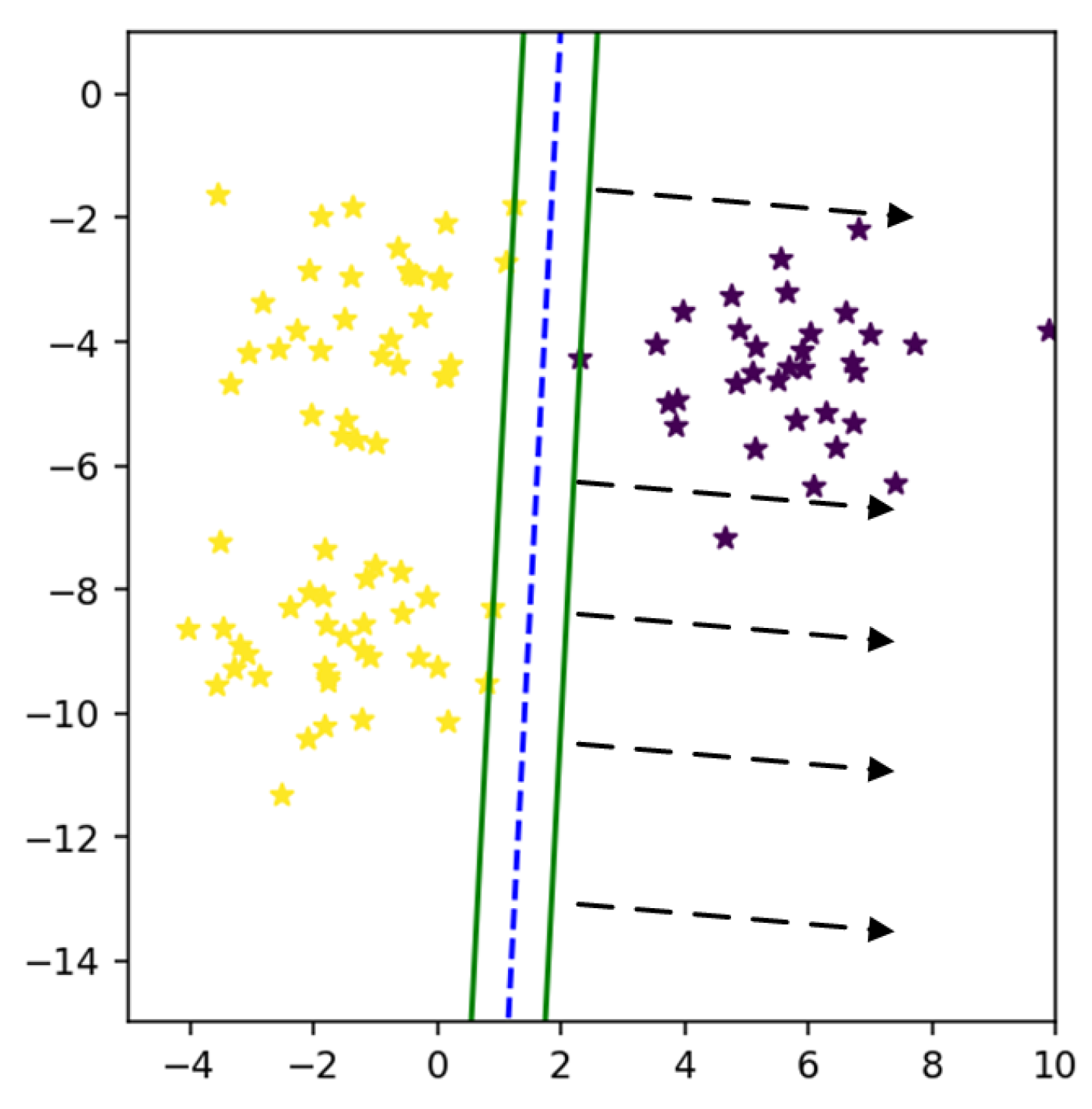
Most of the real-world datasets are not linearly separable; therefore, it is needed to draw a non-linear boundary. In case of non-linear datasets, two types of solutions can be adopted. One is to use soft-margin SVM to accept some errors, and another is to draw a non-linear boundary. Linear separability of the data can be affected by a single point. Even a single sample in the dataset can affect the hyperplane of the SVM. If the data is sensed from sensors, then a single incorrect datum can make the dataset non-linear [16], as shown in Figure 1.

Linear separability can also be applied to check the non-linearity of the data before using SVM as a classifier. SVM with the linear kernel can be applied to the data for linear separability check. By getting 1.0 accuracy on training data, the data are linearly separable, and we can go for hard margin SVM. If the accuracy value is less than 1.0 but in an acceptable range, the soft margin SVM can be applied by accepting some errors (5).

$$y_i(w.x_i+b)\ge 1-\xi {\forall }_i$$

(5)

Here the $\xi >0$ variable relaxes the constraints given in (4). The objective function becomes

$$\begin{array}{c}\hfill minimize{w}^{T}w+C\sum _{i=1}^m{\xi }_i^k\\ \hfill Subjectto{y}_i(w.x_i+b)\ge 1-{\xi }_{i}and{\xi }_i\ge 0;(i=1\cdots m)\end{array}$$

(6)

With the same problem, i.e., non-linear dataset, the classification method can also use kernel tricks to classify the data in kernelized feature space. These kernel tricks transform the data from the original to a kernelized feature space. Among all types of kernels, RBF (7) and polynomial kernels (8) are the most famous [17].

$$K(x_i,y_i)=exp(-\gamma \Vert x_i-x_j{\Vert }^2)$$

(7)

$$K(x_i+y_i)={(x_i.y_i+1)}^d.$$

(8)

In RBF, the parameter $\gamma$ is used to scale the mapping, and in the polynomial kernel, d is the degree of the polynomial. Typically, RBF outperforms as compared to polynomial kernel.

Feature transformation techniques can also be used in non-linear datasets and SVM to transform data into different feature spaces and try to set a hyperplane [18].

$${\mu }^{T}Ax+b,$$

(9)

where A is a transformation matrix, ${\mu }^T$ is weights vector, x is input, and b is a bias.

Along with the feature transformation, another strategy that is used with SVM is metric learning. To learn a linear transformation matrix, which is available more than once, metric learning can be used [19,20]. The researchers used a straightforward approach to deploy the transformation by combining metric learning and SVM. This approach is unable to produce satisfying results, however. Therefore, to integrate metric learning with SVM, many approaches have been proposed, e.g., Metric Learning with SVM (MSVM) [19] and Support Vector Metric Learning (SVML) [21]. There was a limitation with SVML; it only works with a Gaussian radial basis function kernel (RBF_SVM) and ignores the information of radius, while, on the other hand, MSVM [19] was nonconvex.

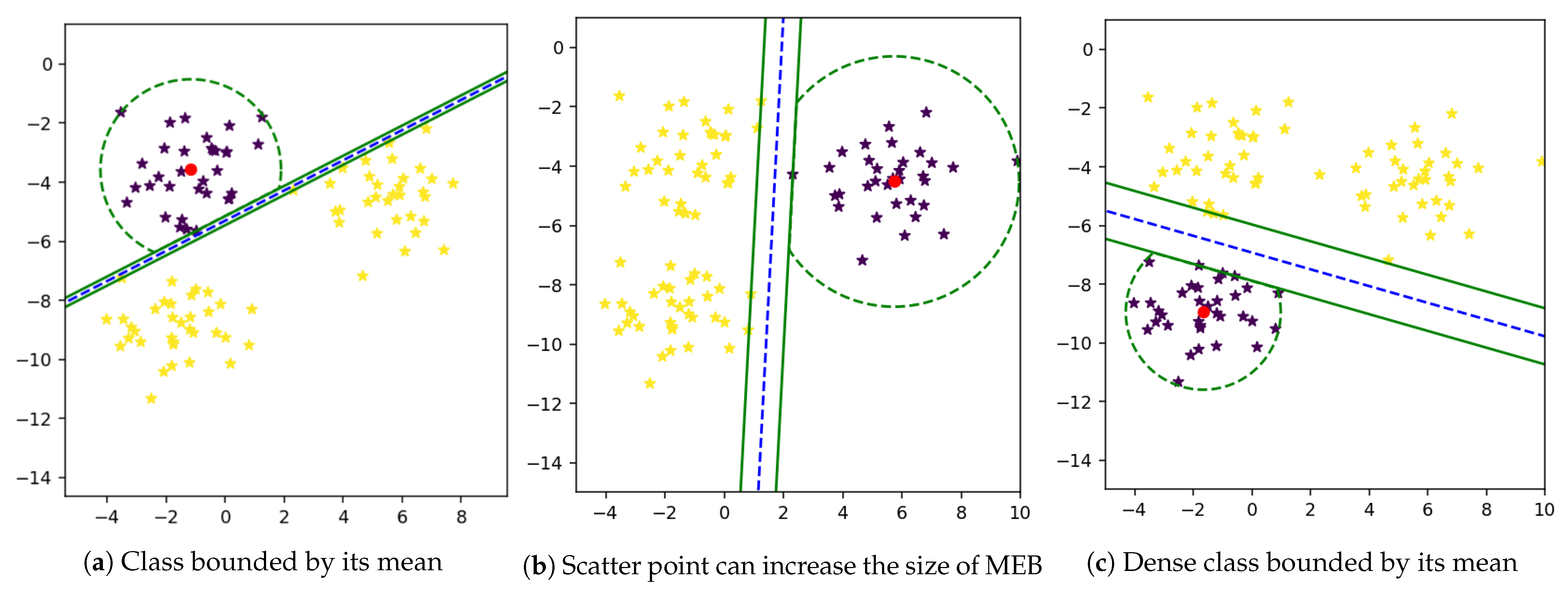
SVM and its extensions are best to cused lassify the data, but the boundary within a class is not enough to achieve higher prediction accuracy. Each class should be bounded in its limited area. To do so, F-SVM [14] proposed a method to bound the class in its narrow region. Mean strategies were used to calculate the radius of the MEB of the class. However, the mean can shift to a dense area of the class. Real-world datasets are with mixed behavior; some classes may be closed and others or scattered. In this case, the value of radius calculated by the mean will be very high. As a result, the MEB can cross the hyperplane or can overlap samples of other classes.

In this paper, a weighted mean approach is proposed to enhance the performance of F-SVM. The F-SVM method computes the MEB of the class by calculating the mean of samples, but the mean can shift to the dense area of the class. If a class contains scattered points along with the dense area, then the radius (maximum distance from mean to samples) will be higher. While the proposed model is based on two steps, the first is the computation of the SVM classifier, and the second is the calculation of the weighted mean. In the first stage, conventional SVM is applied to get the classifier’s parameters; after that, the mean of the class is computed. The distance of the sample from the mean is used as the weight of the sample. By assigning the weight to each instance, the samples show different behavior in the weighted feature space. Now the mean is computed in weighed feature space; thus, the mean shifted to the scattered area of the class. The radius calculated by the weighted mean is always less than the radius by mean. Finally, the size of MEB is reduced. The proposed model named WR-SVM is compared with existing margin radius methods, i.e., F-SVM [14]. The proposed model will use the same parameters on which F-SVM was trained. The 10-fold strategy is used to train and test the model.

The core contributions of the proposed research study is followed:

• Calculate a tighter bound of MEB by using weighted mean.
• By using kernel tricks, non-linear data can be linearly separable, due to which we find w and b with the optimal solution in weighted feature space.
• Proposed model is evaluated on 9 different benchmark datasets and one synthetic dataset, and results are compared with traditional SVM and margin radius-based F-SVM.

2. Related Work

SVM initially was proposed by Vapnik and his team in 1990 [22]. The concept of SVM is derived from neural networks, or we can say that SVM is a mathematical extension of neural networks. Both linear and non-linear datasets can be classified by SVM [23]. SVM performs classification by transforming data into different feature spaces and construct hyperplane on higher dimensions.

SVM finds w and b to set optimal hyperplanes in feature space in the binary class.

$$D_{w,b}(x)=w\phi (x)+b,$$

(10)

where w and b can be determined by Lagrange’s multiplier [24]. The decision rule of SVM is, if $D_{w,b}>0$ then classify as positive otherwise negative class.

As we know in the binary classification problem, the training samples and the classes are given, and they all belong to $R_d$, where the class labels are given as $+1,-1$. SVM can be used for feature selection. Parameter optimization and feature selection are two primary perspectives to enhance the performance of the classifier. An innovative method based upon the genetic algorithm (GA) for feature selection and parameter optimization of support vector machine (SVM) is introduced to enhance the hospitalization cost model’s prediction accuracy [25]. Another technique [26] presents a different feature adoption method to deal with machine learning’s two main issues: class imbalance and high dimensionality. The proposed fixed strategy punishes the feature set’s cardinality via the scaling factors method also is applied with two support vector machine (SVM) formulations intended to deal with the class-imbalanced problem, namely Cost-Sensitive SVM and Support Vector Data Description. A lot of work has been done on feature selection by using SVM [27,28]. In [16] the author proposed a model called SVMRFE. They use the smallest weight to eradicate the features.

SVM features selection method used for prostate histopathological grading. Features selection is mainly used for diagnosing histopathological images [29]. In this study, they use textual features that were obtained from nuclei cytoplasm and stroma. The first step of methodology was to categorize the tissue images. Based on the text of a single classifier and then ensemble learning model was applied by combining the values obtained by each classifier. For that purpose, they use SVM-RFE (Recursive Features Elimination) that integrates SVM-RFE with Absolute Cosine (AC). The results obtained by SVM-RFE (AC) were better than the results of simple SVM.

SVM is used in real-life problems due to its strong kernel tricks. SVM with multi-domain features used for diagnosing rolling bearing [30]. Sensitive features extracted from the highly vibrated signal are still challenging tasks and for diagnosing rolling bearing. An existing classifier that uses single domain features is easy for extraction and recognition of low accuracy. To address this challenge of low accuracy, they proposed a new approach called SVM with multi-domain features that are consist of three stages, i.e., is features extraction, feature selection, and feature weighting. In [31] author proposed Digital Signal Processing platform and PCA-SVM Algorithm for rapid beef meat freshness prediction and identification. They used PCA and kernelized SVM algorithm and embedded system by DSP. In [32], the authors have used kernelized SVM for determining the effectiveness of treatment of tuberculosis. They used SVM to check the effectiveness of the drug. Traditional doctors provide solutions to these problems only on their own experience. Multiple real-life problems in the field of medical and signal processing have been solved by SVM.

Intra-class validation and intra-class ambiguity in the feature space was tackled and resolved by [33]. The concept of large margin and local estimate classification was used. Most of the time, SVM was applied after feature selection. The concept of a single large sparse autoencoder for feature learning was used in [34] and then SVM was applied for classification. SVM performs well but on a small number of samples. In [35] author proposed a new model for feature extraction and classification using SVM. Different features are extracted, combined, and then the similarity is computed by SVM. In [36] SVM was used for tongue image classification. The main problem of this research was to extract features of the tongue. These features are extracted by the Histograms of Oriented Gradient (HOG) concept [37], and then SVM was applied to classify. Experiment results show good classification and prediction results.

Reduced SVM (R-SVM) is proposed by [38] they select features by minimizing $\frac{R^2}{\gamma }\sigma$. They used the SVM radius margin ratio for selecting features. This model was used to optimize the radius margin bound. Moreover, the authors first scaled a feature by multiplying each feature by a vector $\sqrt{\mu }$, and then SVM is applied to these resulting features. The resulting feature space is not the same as the original feature space. Due to this, in resulting feature space classes are more linearly separable than the actual feature space. The radius of feature space after transformation was denoted by $R_{\mu }$. In R-SVM, two-step classification was performed; in the first step, SVM is used to select features, and then the radius margin is optimized by using extended feature space. They aimed to achieve a better generalization error. For achieving this aim, they optimize the radius margin, which accomplishes the following optimization problem.

$$\begin{array}{c}\hfill \begin{array}{c}min\\ w,b,\mu ,R_{\mu }\end{array}=\frac{1}{2}{\Vert w\Vert }_2^2{R}_2^{\mu }\end{array}$$

(11)

where $R_{\mu }$ is computed by Vapnik 1998 [39]. The constraints involved to restrict the parameters of (11) are

$$y_i(w,\sqrt{\mu }+b)⩾1,{\forall }_i$$

where $y_i$ is the label, w and b are classification parameters. The value of $\mu$ is restricted by another constraint which was

$${\displaystyle \sum _{k=0}^d{\mu }_k=1,{\mu }_k⩾0,\forall K}$$

The smooth feature selection was performed through this optimization problem. It had the main limitation that it is not convex. To eliminate this limitation, an upper bound of the objective function was proposed [40].

$${\mu }_k{R}_k^2⩽R_{\mu }^2⩽\sum _k^d{\mu }_k{R}_k^2$$

(12)

By using this upper bound, the optimization problem becomes convex.

The radius margin error bound not only separates the class from all others but also restricts it within a bounded area. For $x_i$ training samples given a feature mapping $\Phi :x\mapsto \mathcal{H}$, to transform the features space $\mathcal{H}$, the radius of MEB according to [41] in that extended feature space is given by

$$\underset{R,x_0}{min}{R}^2,s.t.{\parallel \Phi (x_i)-\Phi (x_0)\parallel }_2^2\le R^2{\forall }_i$$

(13)

Another solution to minimize the area of MEB is proposed by [42]. The authors proposed two variants of SVM, $R-SV{M}_{\mu }^{+}$, and $R-SV{M}_{+}$. $R-SV{M}_{\mu }^{+}$ was a non-convex and difficult to solve because of radius constraints. It was based on R-SVM, in which the ratio of the optimization problem replaces the sum. It first determines the transformation matrix and then projects it into a new feature space.

$$\begin{array}{c}\hfill \underset{w,\xi ,\mu ,b,R_{\mu },x_0}{min}\frac{1}{2}{\parallel w\parallel }_2^2+\lambda R_{\mu }^2+C\sum _i^l{\xi }_i\\ \hfill s.t.y_i(〈w,D_{\sqrt{\mu }{X}_i}〉+b)\ge 1-{\xi }_i,{\forall }_i\\ \hfill \sum _{k=1}^d{\mu }_k=1\mu ,\xi \ge 0\\ \hfill \parallel D_{\sqrt{\mu }{X}_i}-D_{\sqrt{\mu }{X}_0}{\parallel }^2\le R_{\mu }^2,{\forall }_i\end{array}$$

(14)

The radius constraints here were non-convex, and the optimization problem was difficult to solve.

On the other hand, $R-SV{M}_{+}$ was a metric learning-based extension of SVM. In this algorithm, a matrix D is used to transform features, and SVM is used to classify the data in that new feature space. The extended feature space is also used by [43] in which the author used LogDet regularization with SVM, called LSVM. The methodology was based on the two-step minimization strategy, where the first is to use LogDet to regularize the feature space and then compute the radius. The radius computation method was the same as F-SVM, which was the mean of the class.

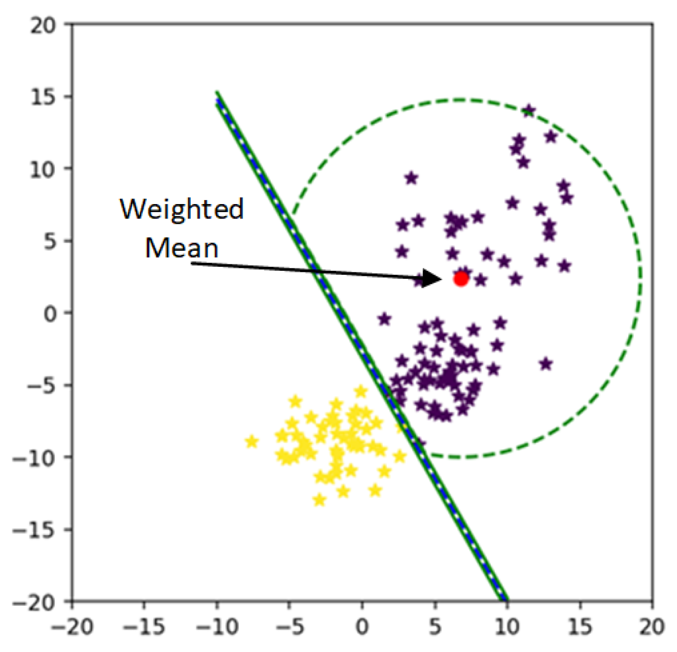
An extended version of SVM is proposed [14] to reduce the value of the radius of MEB. According to F-SVM, a class area is a maximum distance from the mean to any sample. If we have scattered data, the mean of a class shift to higher values due to which a point is so far from a mean. As a result, we get a higher value of the radius, and MEB becomes very large, as shown in Figure 2. MEB bound the class area within a specific limit and restrict the samples to be in a particular range. By limiting the instances of one class in a particular region, the performance of SVM is improved. The proposed section will discuss the impact of MEB on results.

In F-SVM jointly learn the feature transformation and a classifier. F-SVM proposed a new bound of MEB. Where radius of MEB is bound by R which is

$$\frac{1}{2}R⩽R⩽\overline{R}$$

(15)

where,

$$\overline{R}=ma{x}_i{\Vert A{x}_i-A\overline{x}\Vert }_2^2$$

(16)

The authors computed each point’s distance from the mean value, and then the radius is the maximum value from the vector of distances. Here they got the Radius of MEB.

The computed radius was biased to the dense area of the class and had a large value in the case of scattered points. The mean strategy of computing the radius of MEB will always move to the dense area. To reduce the size of MEB, the proposed method introduces the weighted feature space and calculates the radius of MEB from that space. As a result, the size of MEB is reduced. By reducing the size of MEB, the area covered by the class is decreased.

3. Proposed Methodology

Experiments are conducted on different benchmark datasets. The performance of WR-SVM is compared with F-SVM, which was the recently proposed radius margin technique. WR-SVM learns classifiers such as w & b and then weighted mean of the class simultaneously. The classifier attributes are first used to classify the data in the case of the linear kernel. In contrast, in the case of RBF, kernel data are transformed into feature space, and the classification is applied to that extended space [44].

In the first stage, after loading the data into the simulation environment, the linear separability of the data is checked to reduce execution time. For this purpose, SVM with the linear kernel is used by applying one vs. all techniques for all experiments. The linear separability allows us to apply either soft margin SVM or hard margin SVM.

In the first stage of experiments, SVM is applied to check the linear separability of the data [45]. Based on the separability check result, either soft margin SVM or hard margin SVM is applied.

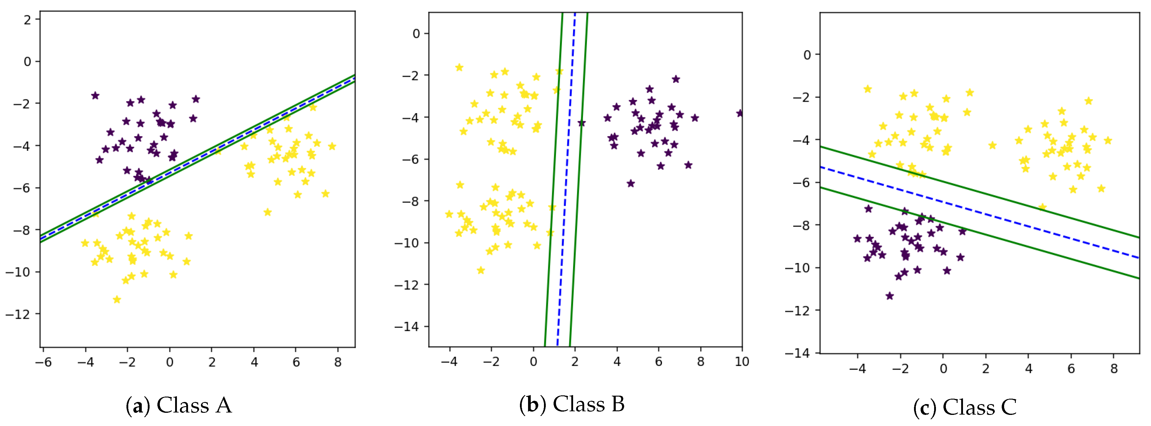
There are multiple classes in single feature space in a multi-class problem, due to which samples of one class may overlap another class [46]. Therefore, there is a need to separate these classes in a way that the maximum prediction accuracy will be achieved. The multi-class problem can be solved using the one-vs-all technique. It is not easy to find out a mathematical equation that separates all classes from one another. In many cases, it is not possible to find an optimal solution. In the One-Against-All technique, firstly proposed by Vapnik in 1995 [16], one class is classified from all other classes. First, we computer w and b and then draw a hyperplane between one and all other classes using these weights and bias as shown in Figure 3a–c.

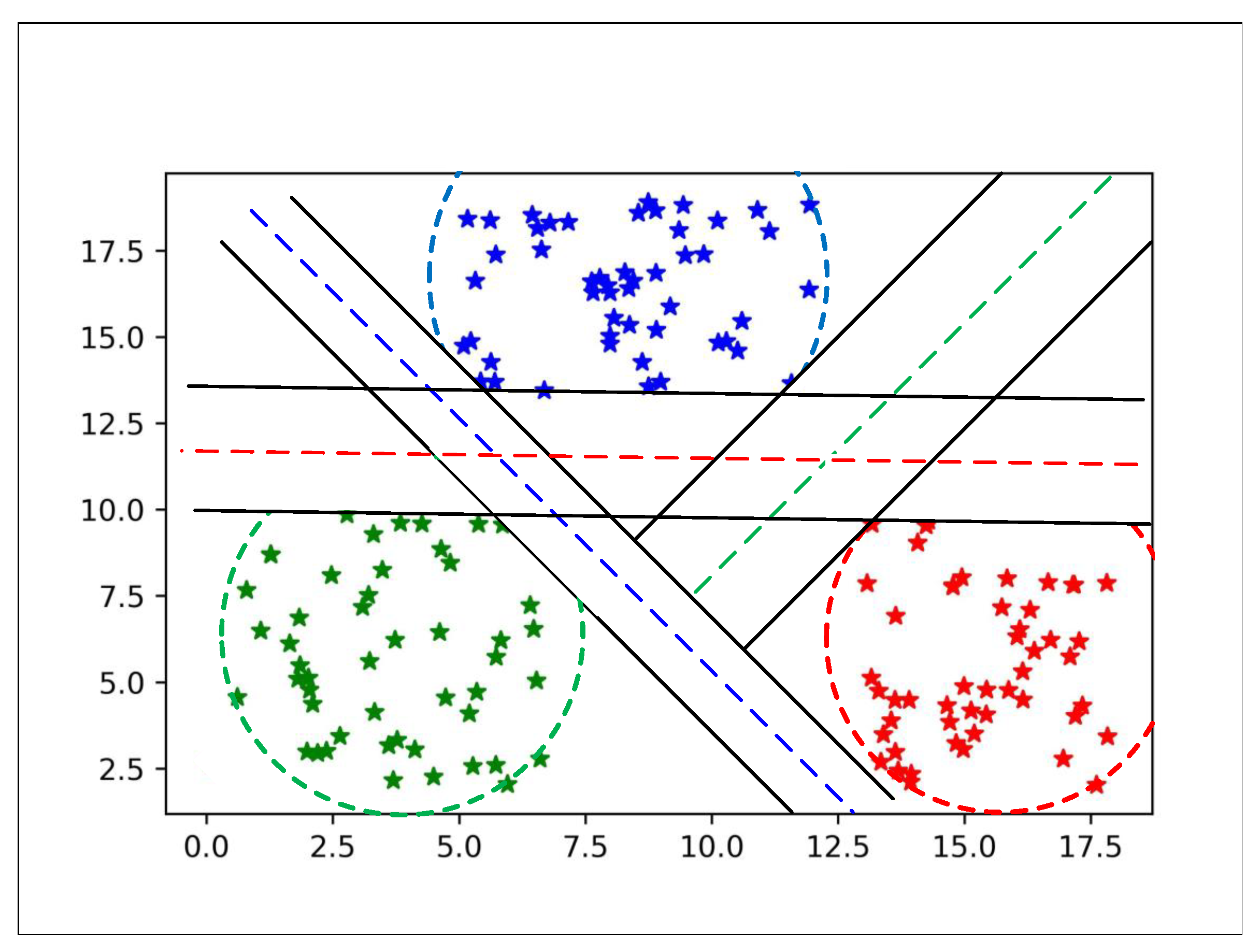
After finding these hyperplanes between classes, we set all hyperplane in one plot to show separability between all classes as shown in Figure 4.

Next, each class sample should be bounded in an enclosing ball. To do the task, initial mean is computed, and the radius of each class is calculated to draw MEB.

According to [40], the upper bound of the radius-margin is bounded with $ma{x}_k{\mu }_k{R}_k^2⩽R_{\mu }^2⩽{\sum }_k{\mu }_k{R}_k^2$ where $R_k$ is the radius of dimension k. Ref. [42] proposed a tighter bound for the radius-margin, where

$$R_o⩽R_{\mu }⩽((1+\sqrt{3})/2)R_o$$

(17)

However, the experiments are restricted to only linear feature space. The kernelized features space is not used to compute the radius. While the proposed technique first transforms the data into kernelized feature space, and then the radius of the MEB kernelized feature space is transformed into weighted kernelized feature space.

3.1. Minimum Enclosing Ball of F-SVM

According to F-SVM the radius of MEB is bounded by $\overline{R}$ (15). The mean of a class is not a solution to get the tighter upper bound because the mean can shift to higher values. After applying the conventional SVM and initializing the classifier attributes, the mean of class is computed $\overline{X}=\frac{{\sum }_{i=1}^n{x}_i}{n}$. If we calculate the distance of mean from all samples of class, then according to F-SVM, the radius of MEB is:

$$\overline{R}=ma{x}_i{\Vert A{x}_i-A\overline{x}\Vert }_2^2$$

(18)

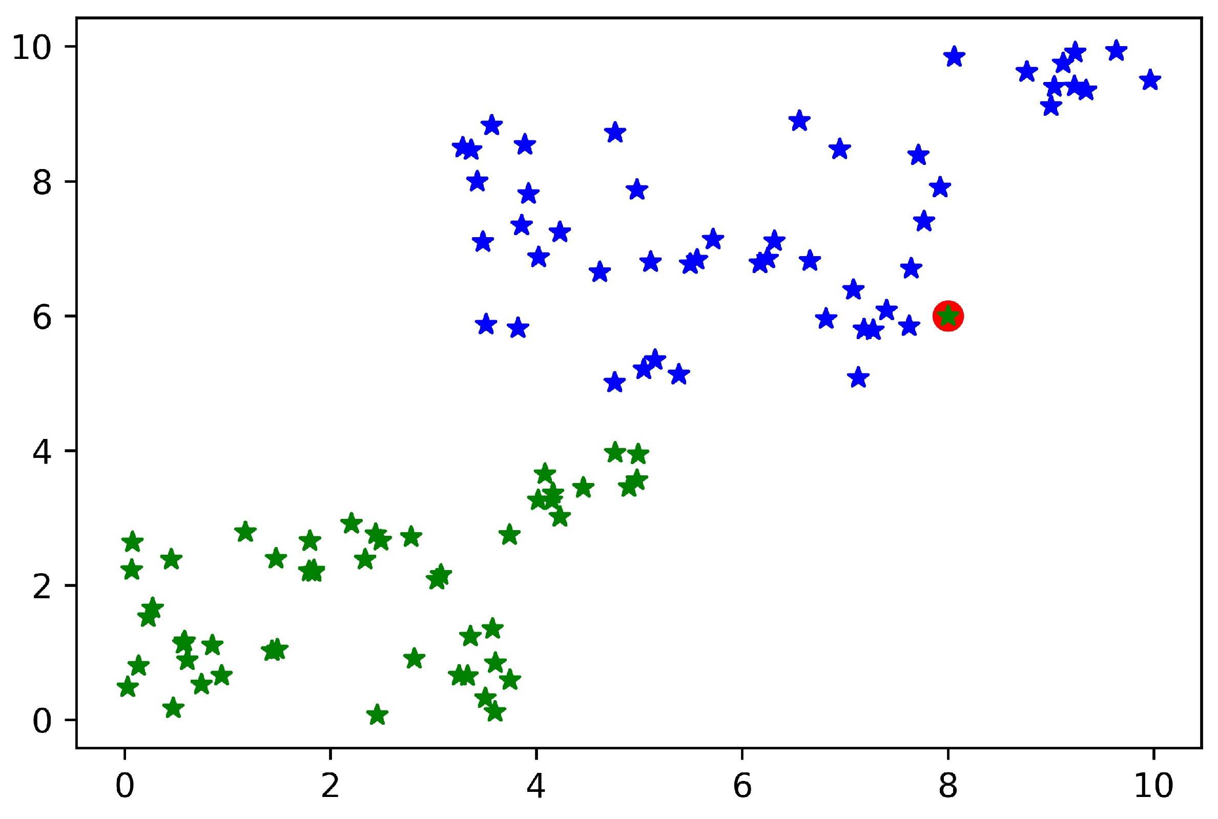
If we have more than two classes, then the radius is essential because each class should have its bounded area. However, in the binary class problem, one side of the hyperplane is occupied by one class, as shown in Figure 5. So, we need to bound the class area because when we have anomalies in test data or a new class emerging in actual data, we should have an enclosed space for both classes.

The radius of MEB according to F-SVM is given in (18) and Figure 6 shows the bounded a rea of class using its mean. It is clear from the figure that the mean of the class is shifted to a dense area, due to which area of MEB is increased. It might be possible to have anomalies in the data in scattered form. By predicting the test data using the classifier and MEB of F-SVM, the higher chances are the model predicting the anomalies as a positive sample. If a large number of outliers are in the class, the prediction accuracy can be very low.

The main problem with the radius computed by (18) is that it cannot deal with the anomalies and scatter points of the class. Because of the higher value of the radius, MEB can cross the separating line or hyperplane in multi-class problem [47]. When the MEB cross the hyperplane, samples from other class can also be in the area of MEB that cross the line. Similarly, in the case of the multi-class problem, more than one class can be in one MEB. The proposed technique of computing MEB also restricts the MEB on one side of the hyperplane.

3.2. Proposed Minimum Enclosing Ball

In the proposed method of calculating the minimum enclosing ball, a weighted mean is calculated instead of a mean. Firstly, SVM is applied to compute the classifier attributes, i.e., w and b. Secondly, the mean of each class is calculated by using the same method adopted by F-SVM, i.e., Euclidean distance. As the time complexity of SVM is $O(n^2)$.

In the proposed method, a weighted mean is calculated instead of a mean. First, F-SVM followed by SVM is applied to get the MEB of SVM. After that, the weighted mean is computed, where the weight of each sample is its Euclidean distance from the mean of class, as shown in (19). The selected square Euclidean distance allows us to get the weighted feature space based on the distance of each sample from mean to samples. Moreover, it is observed that the additional iterations of the weighted feature space lead to the same result due to the choice of weight based on the square of the Euclidean distance. These weights are calculated in kernelized feature space, whereas F-SVM uses these distances as the radius of MEB, as shown in (18).

$$weight{x}_i={\Vert \overline{x}-x_i\Vert }_2^2$$

(19)

After calculating the weight for each sample. Weighted features are calculated by using (20). The weight of each sample is added to all the samples of the class.

$${\overline{x}}^{(w)}=\frac{{\sum }_{i=1}^n{x}_i.weight{x}_i}{{\sum }_{i=1}^{n}weight{x}_i}$$

(20)

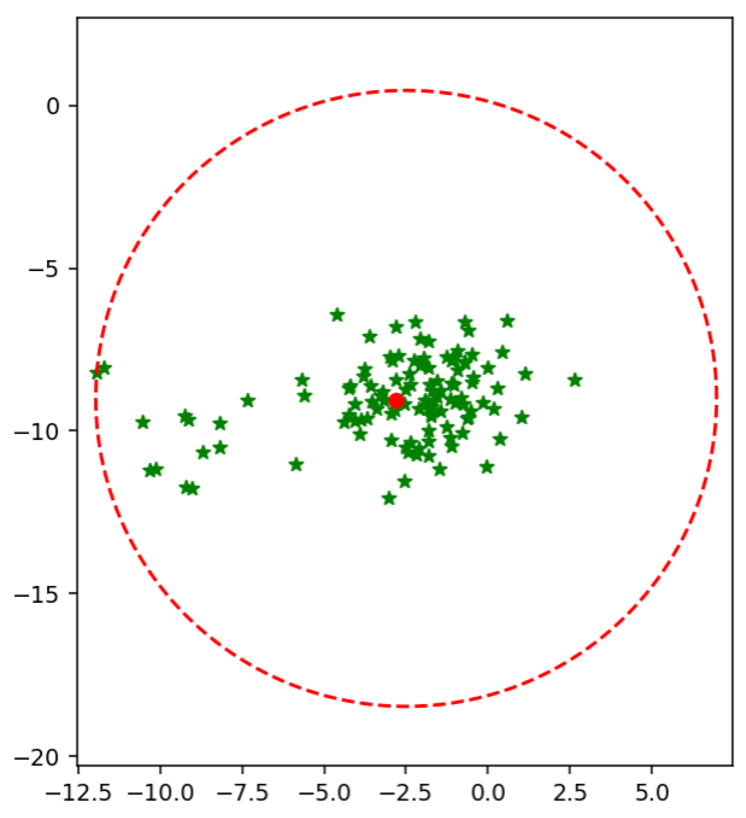
After assigning weights to each sample, all the class points are shifted from kernelized feature space to weighted kernelized feature space. By approaching the weighted feature space again, the mean of the weighted feature space is calculated. The mean of weighted feature minimizes the MEB radius of each class as shown in Figure 7.

After calculating weight for each sample from (19) and then weighted samples from (20), the mean of the class shift towards scattered points of the class, as a result, our radius of MEB is minimized.

The weighted mean for the multiclass problem using one vs all technique is illustrated in Figure 8a–c. Furthermore, the MEB crosses the separating line; these points of MEB are excluded by calculating the circumference of the MEB. All the points which do not satisfy the constraint given in (4) are excluded from MEB.

3.3. Flow and Mathematical Model of WR-SVM

The proposed model accepts the data and applies pre-processing techniques to make it classifiable by the model. The flow model of WR-SVM is given in Figure 9. First, the data are encoded by using an ordinal encoder. Some dataset features are alpha-numeric; therefore, to perform the calculations on the data, attributes are encoded into numeric values. After that, data are divided into 10 folds to apply classification by selecting one as a test fold and the remaining as training. Instead of applying soft margin SVM or hard margin SVM directly, the linear separability is checked, and the decision is made based on the accuracy value. SVM with the linear kernel is used to check the linear separability of the data. If the accuracy value on training data is 1 then the data are linearly separable; otherwise, data is not separable.

In case of Hard margin SVM each sample should satisfy the constraints given in (2) and (3). The hard margin SVM strictly draws a line; if the data are separable, then return the value of w and b. By applying the soft margin SVM, the value of the slack variable is selected to accept some error. Next, the kernel is selected based on the accuracy value achieved in the separability test. The kernel tricks transform the data into a kernelized feature space and classify the data in that space. The one-vs-all technique is used to classify two classes at a time. One class is separated from all others and assigned a label as 1. Similar samples of other classes are merged and assigned a label as $-1$. Now, the problem is converted from multi-class to binary class. Other classes are selected iteratively one by one. All the weights are saved for each class and used at the time of testing. In both cases, soft margin SVM and hard margin SVM, the feature space is passed to the next phase. In that phase, the MEB of the class is computed, which is the core idea of WR-SVM. First, the mean of class and the Euclidean distance of samples from the mean is computed. After that, the distance matric is used as the weight of samples. The kernelized feature space is moved to the weighted kernelized feature space by assigning the weights to the samples. The mean of each class in the new feature space gives us a minimized radius value compared to kernelized feature space. The MEB with the computed radius is drawn on the original feature space. Using radius and mean value, we compute circumference points of the circle and exclude all those points that belong to another side of the hyperplane. WR-SVM is based on two steps: the classifier and calculation of the MEB radius as shown in Algorithm 1.

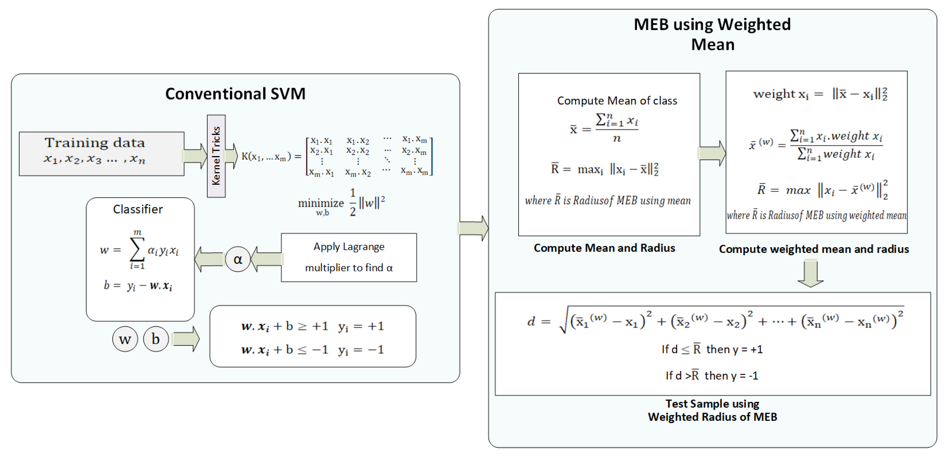
The mathematical model of WR-SVM is illustrated in Figure 10. First, the data are pre-processed and divided into k-folds, as discussed earlier. The processed data are passed to conventional SVM by selecting the kernel function, which changes the datas’ dimension. Lagrange Multiplier [48] is used to find the value of $\alpha$, which is used to find the value of w and b in the next step. The classifier values i.e., w and b are used to classify the test data, as shown in (2) and (3). Next, the radius of MEB is computed in three steps. Firstly, the mean of each class is computed, and the radius according to F-SVM is computed. Secondly, the distance of each sample from the mean is computed, which is used as the weight of that sample. The weights are assigned to each sample, and the weighted mean is computed. From the weighted feature space, again, the radius is computed. The radius which is computed from the weighted feature space is minimized. For the test samples, first, w and b are used to predict the class of samples, and after that distance of that test, the sample is computed from the weighted mean of the sample. If the distance is less than the radius of class, i.e., $\overline{R}$, then the sample belongs to $+1$ and $-1$ in other cases.

Algorithm 1: The two-step minimization algorithm for WR-SVM.

4. Experimental Results and Analysis

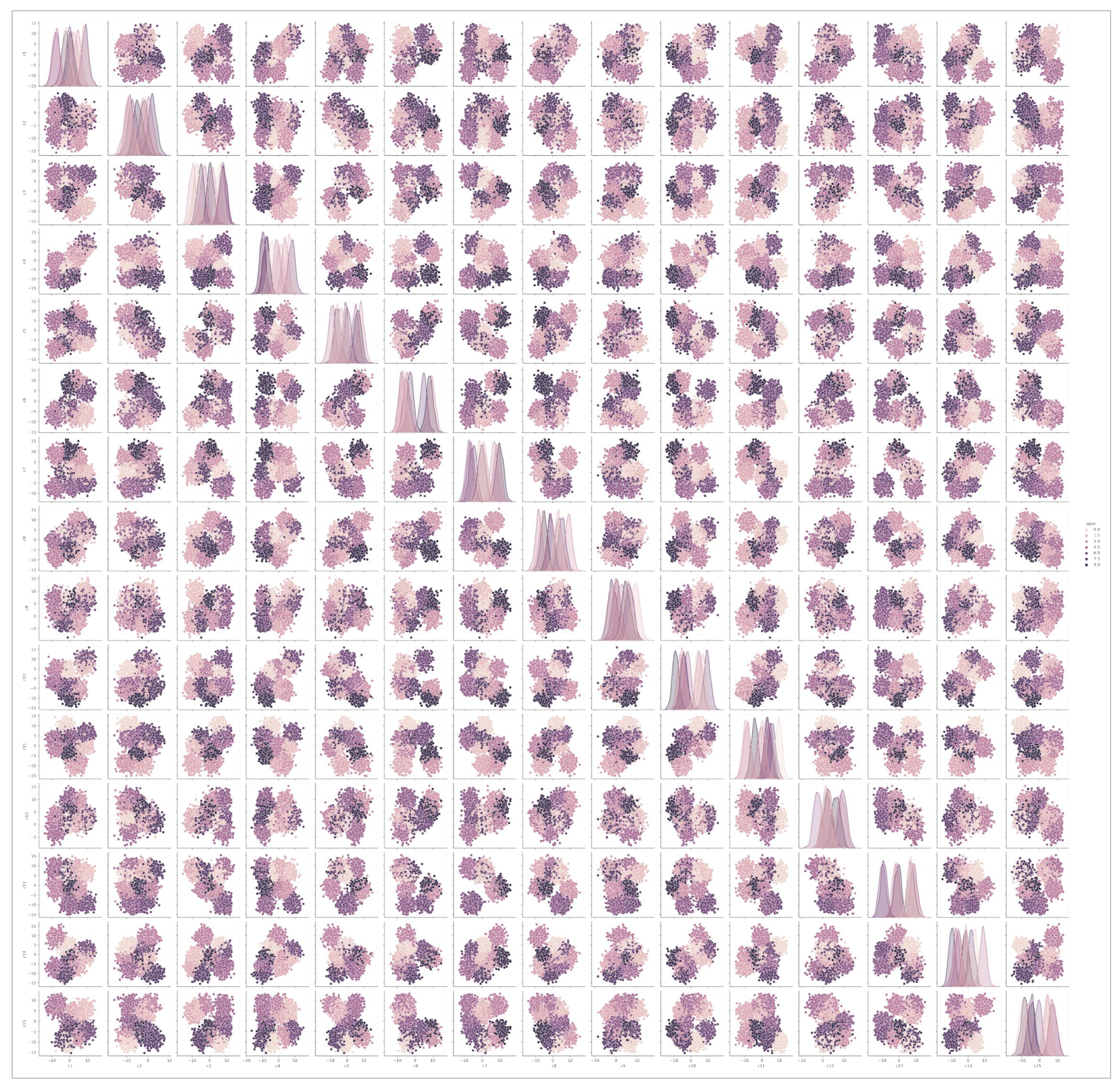
Multiple benchmark and one synthetic dataset (https://github.com/atifrizwan91/Synthetic-Dataset/blob/main/synthetic-dataset.csv, accessed on 3 April 2021) is used to evaluate the performance of proposed model. All the features of synthetic dataset are visualized in the Figure 11 and the datasets are listed in

Table 1. Description of the 10 UCI datasets used in experiments.

ID	Dataset	# of Samples	# of Classes	# of Dimensions
1	Iris	150	3	4
2	Waveform3	5000	3	21
3	Glass	214	6	9
4	USPS	9298	10	257
5	Synthetic	5000	10	15
6	Segment	2310	7	18
7	Sonar	208	2	60
8	Musk	6598	2	166
9	Zoo	101	7	16
10	Breast Cancer Dataset	277	2	9

. The results are compared with conventional SVM and F-SVM in terms of accuracy. As it is clear from Table 1 that all datasets have different numbers of samples, dimensions, and classes. The reason for selecting these datasets is that the results of MEB-based F-SVM are also reported based on these datasets. All the datasets are best to evaluate and compare the performance of the proposed model. The synthetic dataset is generated by using the library of python called Keras.

The parameters of the data generator are set in a way that there is no linear separability between the classes of the data. The relationship between all features of synthetic data is given in Figure 11. It is clear from the illustration that there is no linear separability between any feature of the dataset. Furthermore, the number of synthetic dataset samples is also high compared to all other benchmark datasets.

To measure the effectiveness of our proposed solution, we compared our results with F-SVM [14]. For a fair comparison, we employed accuracy as a performance evaluation measure similar to the case of F-SVM. The proposed model is evaluated on both Linear and RBF kernel, and results are reported based on accuracy. All the benchmark datasets are openly available and discoverable online on the UCI machine learning repository. The results of WR-SVM based on linear kernel and RBF kernel is shown in

Table 2. Comparison of the average classification accuracy (%) of Linear WR-SVM by Linear SVM and Linear F-SVM.

ID	Dataset	SVM	F-SVM	WR-SVM
1	Iris	96.67 ± 0.34	98.00 ± 0.56	98.90 ± 0.23
2	Waveform3	87.40 ± 0.59	87.80 ± 0.31	88.86 ± 1.05
3	Glass	66.36 ± 0.98	70.45 ± 0.74	72.15 ± 0.67
4	USPS	97.89 ± 0.21	98.80 ± 0.10	98.91 ± 0.09
5	Synthetic	83.85 ± 1.7	90.65 ± 0.09	90.86 ± 0.10
6	Segment	90.61 ± 1.06	92.60 ± 0.41	93.4 ± 0.47
7	Sonar	81.43 ± 0.63	85.71 ± 1.17	90.47 ± 0.96
8	Musk	91.98 ± 0.86	92.52 ± 0.91	94.05 ± 0.63
9	Zoo	94.55 ± 1.51	98.18 ± 0.52	98.18 ± 0.49
10	Breast Cancer Dataset	97.36 ± 0.85	98.68 ± 0.13	98.78 ± 0.11

and

Table 3. Comparison of the average classification accuracy (%) of kernel WR-SVM by Kernel-SVM and Kernel-F-SVM.

ID	Dataset	SVM	F-SVM	WR-SVM
1	Iris	96.67 ± 0.41	97.33 ± 0.64	98.12 ± 0.37
2	Waveform3	87.56 ± 1.20	87.64 ± 0.67	88.81 ± 0.91
3	Glass	66.36 ± 1.97	74.55 ± 0.96	74.94 ± 0.96
4	USPS	97.92 ± 0.45	98.85 ± 0.38	98.96 ± 0.42
5	Synthetic	85.67 ± 1.42	92.71 ± 0.49	93.04 ± 0.45
6	Segment	97.36 ± 0.99	98.23 ± 0.47	98.62 ± 0.42
7	Sonar	86.19 ± 1.35	95.71 ± 0.82	97.85 ± 0.93
8	Musk	99.73 ± 0.21	99.86 ± 0.14	99.86 ± 0.16
9	Zoo	93.64 ± 1.39	97.27 ± 0.54	98.03 ± 0.39
10	Breast Cancer Dataset	97.82 ± 0.71	99.18 ± 0.24	99.57 ± 0.15

respectively.

In all types of datasets, WR-SVM’s performance is good compared to conventional SVM and F-SVM. The reason behind this performance is that the proposed model performs one step higher than F-SVM. The performance of WR-SVM cannot be less than the base model in any case because when the data has some scattered points, the performance of the model will be improved and will remain the same in another case.

It is noticed from the experiments that when MEB of both classes overlap each other than some samples of both classes can be in intersected area as shown in Figure 12. The non-linear separating line can classify these points, but it is difficult to draw the non-linear boundary between all classes in the case of a multi-class problem.

To evaluate the performance of the proposed WR-SVM in terms of computational cost, time factor is considered. The big O notation is commonly used time and space complexity measure to illustrate the worst time taken by the algorithm. As the time complexity of SVM for n training samples is $O(n^3)$ while the space complexity is $O(n^2)$. F-SVM takes one step after the classification of the data, which was the calculation of the radius of MEB.

F-SVM takes one step after the classification of the data, which calculates the radius of MEB. The calculation of MEB for n number of classes can increase the time complexity and take more space. While in the case of WR-SVM, the radius of MEB is, and the classification parameters, i.e., w and b, are calculated simultaneously. While calculating the radius of MEB, weights are assigned to each sample, and the weighted mean is calculated. The weighted mean helps the model to reduce the radius of MEB. F-SVM takes the time to calculate the mean of each class, while the proposed method takes the same time to assign weights to each sample. Consequently, the time complexity of both F-SVM and WR-SVM is the same, which is $O(n^4)$.

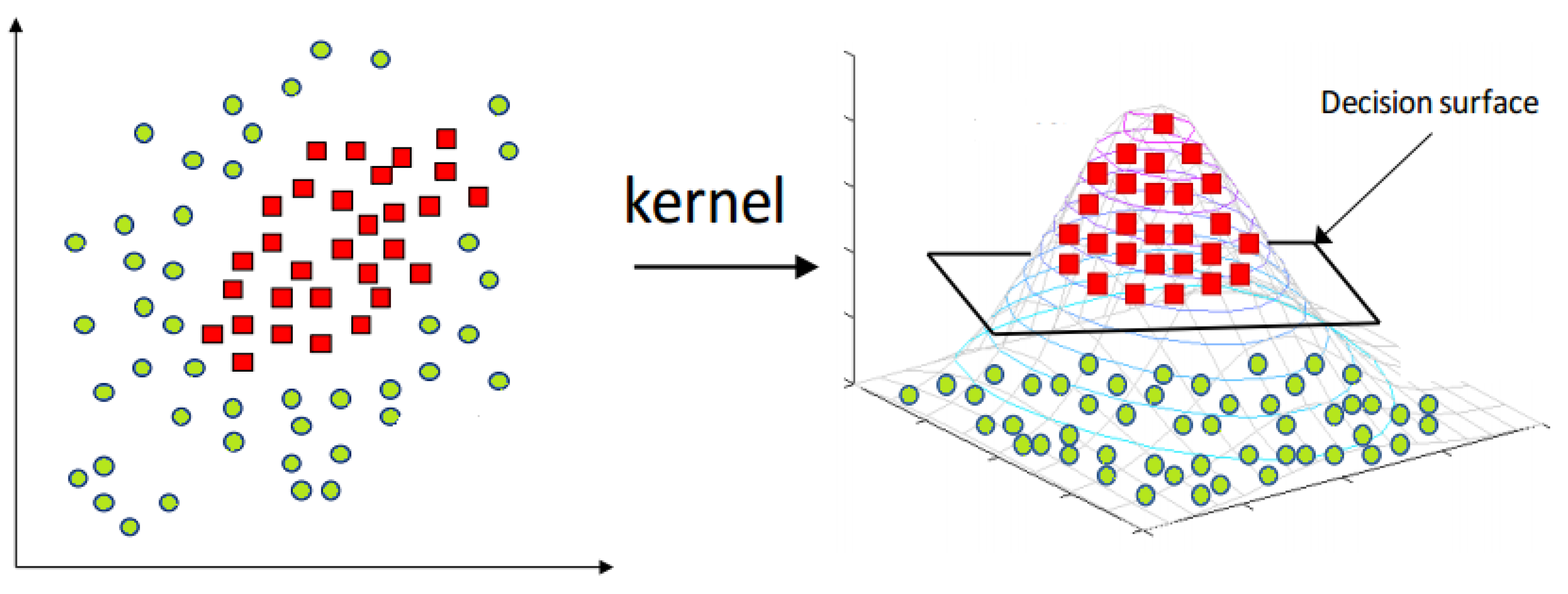
Sometimes, it is impossible to draw the non-linear boundary between two classes in actual feature space, so the kernel tricks can be used to transform the data to another kernelized feature space, as shown in Figure 13. In the case of testing samples, when the data are dekernelized to the original feature space, the testing samples can be located on another side of the hyperplane. So, there is a need for MEB, which encloses the samples within a limited area.

We have performed two sets of experiments in our work. The first step is to classify all samples that are given in the training set. Then the second step is to find the radius of MEB by using the weighted mean of class. Classification is performed on a continuous numeric dataset listed in Table 1. The following steps are performed to classify the data.

• First of all, one class is separated from all others to apply one against all techniques. Here we apply conventional SVM to get the value of w and b such as classifier
• Check whether these two classes are linearly separable or not by applying linear SVM as discussed before.
• Apply a kernel trick to classify the training data in transformed feature space in case of soft margin SVM.

  $$K(x_1,x_2,...x_m)=\left[\begin{array}{cccc}{x}_1.x_1& x_1.x_2& \dots & x_1.x_m\\ x_2.x_1& x_2.x_2& \dots & x_2.x_m\\ ⋮& ⋮& \ddots & ⋮\\ x_m.x_1& x_m.x_2& \dots & x_m.x_m\end{array}\right]$$
• Find the value of Lagrange multiplier ($\alpha$)
• Find the value of w using

  $$w=\sum _{i=1}^m{\alpha }_i{y}_i{x}_i$$
• Find the value of bais (b) using

  $$b=y_i-w.x_i$$
• Repeat Step 1 to 6 for each class of training set.

It is not always possible to get a hyperplane with zero training error so, we go with soft margin SVM by accepting some mistakes. In some cases, we get the hyperplane in acceptable error, but when we have mixed samples of all classes, as shown in Figure 10, then the soft margin will not work in an acceptable range. To solve the mentioned problem, the RBF kernel is applied (7) to transform the data into kernelized feature space.

After classifying data in feature space, we need to bound a class within its area. The weighted mean is computed to get the upper bound of radius, and then the circumference is calculated to get the whole area of the class. Our proposed method targets those samples located in an intersected area of both classes as shown in Figure 12. In Figure 12 the mean of a class is computed to get the upper bound of radius. 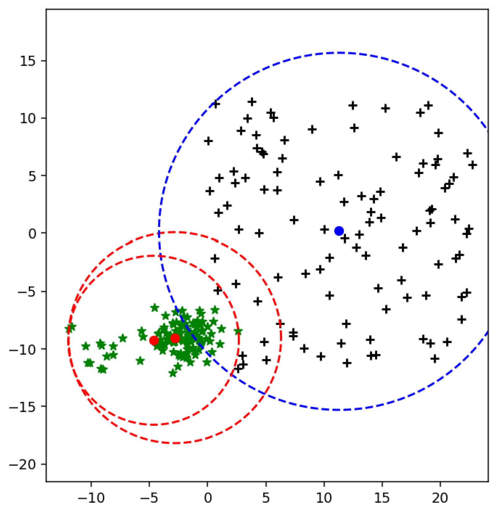Figure 14 shows both mean and weighted mean of class in two-dimensional space. In experiments, all datasets are multi-dimensional. WR-SVM shows improvement in terms of accuracy compared to existing methods such as SVM and F-SVM using linear and RBF kernels.

Therefore, it is noticed that many samples are in the intersected area and far from the mean of its actual class. When weighted mean is used to get the upper bound of class, then it is clear that the number of samples in an intersected area in Figure 14 is less than Figure 15.

5. Discussion

This section presents the comparative analysis of the proposed weighted radius approach and explains how the proposed method shows better results than other margin radius approaches. SVM is a famous and commonly used classification technique because it not only focuses on the separation of the data but also considers the maximum margin between two classes, as shown in Figure 3. Along with the maximum margin, the radius of the class is equally important to be considered to improve the overall performance of the algorithm. To achieve the objective, multiple margin radius-based techniques are proposed, and different radius bounds are presented. 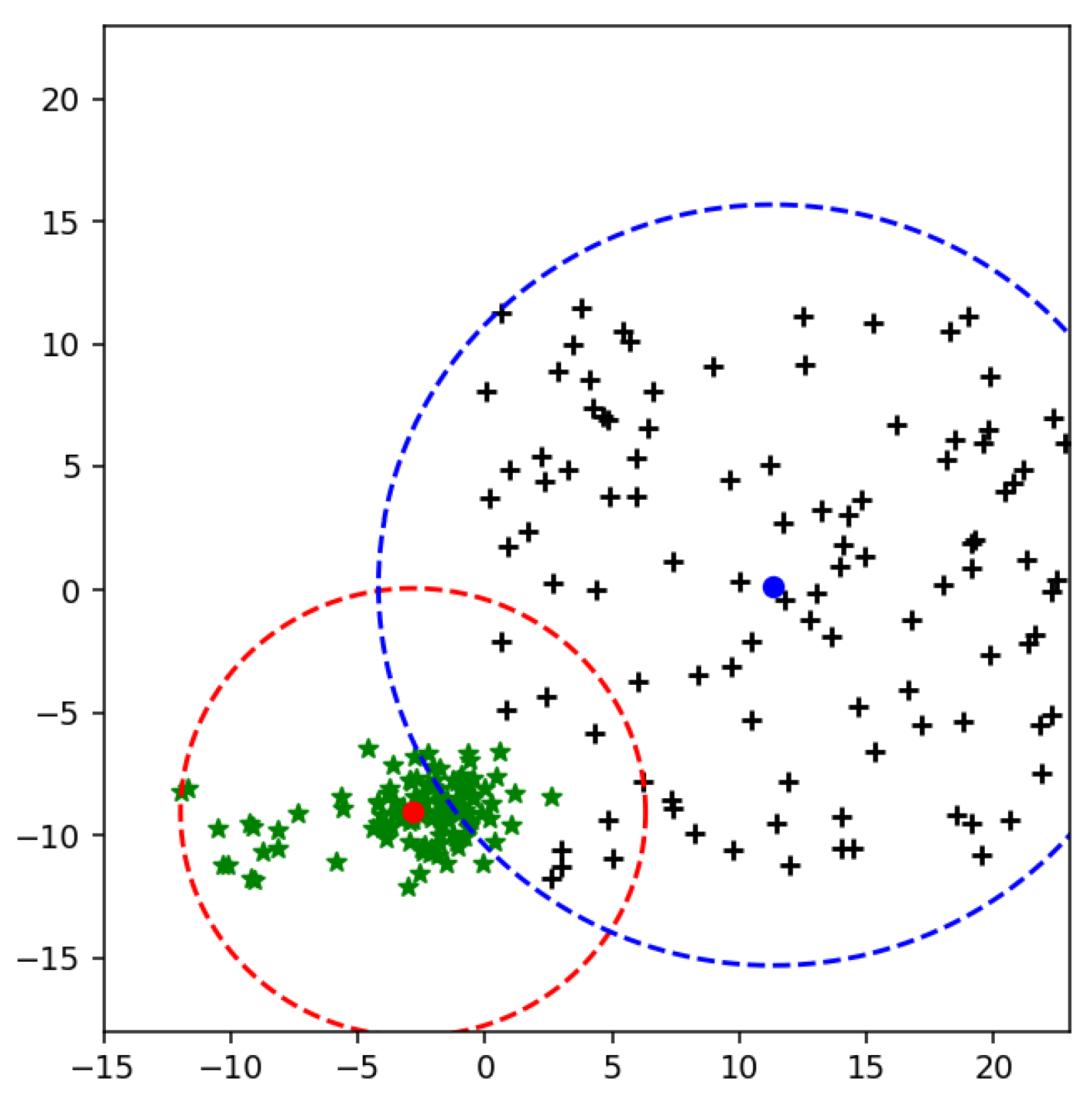The recently proposed margin radius-based approach presented in [14] computes the radius using the mean of the class. The mean can shift to higher values. When the data contain some scattered points, then the radius of MEB will be higher, as shown in Figure 6. Because of the high radius value, the MEB of the class crosses the hyperplane and can also cover the area of another class in binary and multiclass problems. 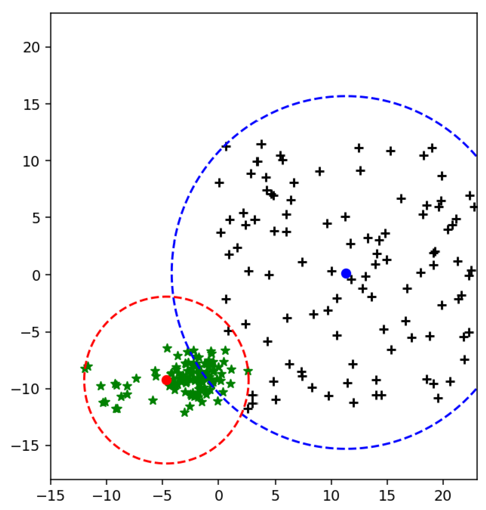As a result, the samples in the intersected area of multiple MEBs can be predicted incorrectly, as shown in Figure 15. To minimize the radius of MEB instead of the mean, the weighted mean of the class is computed. The samples targeted by the proposed methods are scattered points of one class. The proposed solution assigns weights to each class sample based on their distance from the mean value. The scattered samples always far from the mean as compared to the dense area’s points. By assigning the weights to each instance, features are transformed from their original space to weighted feature space. The mean of weighted feature space, for instance, weighted mean, shifts to scattered points of the class. By moving the mean value from dense to scattered points, the radius of the class is decreased. As a result, the MEB of each class is minimized, as shown in Figure 7. Moreover, the area occupied by the proposed MEB is also reduced, and intersected area of multiclass is also decreased. Two-step training of WR-SVM is based on the computation of classification parameters and radius of MEB. After the training phase, when the samples are tested, the SVM classifier is used to classify the sample, and then the radius is used to check whether the sample is within MEB or not. The proposed model compared with F-SVM in terms of the true predicted number of samples for Linear and kernelized feature space as shown in

Table 4. Compaison of F-SVM and WR-SVM in terms of true predicted samples in linear and kernelized feature space for each dataset.

			Linear Kernel				RBF Kernel
ID	Dataset	a ${}^{\mathbf{1}}$	b ${}^{\mathbf{2}}$	c ${}^{\mathbf{3}}$	d ${}^{\mathbf{4}}$	e ${}^{\mathbf{5}}$	f ${}^{\mathbf{6}}$	g ${}^{\mathbf{7}}$	h ${}^{\mathbf{8}}$	I ${}^{\mathbf{9}}$
1	Iris	150	147	148	98	98.9	145	147	97.33	98.12
2	Waveform3	5000	4390	4443	87.8	88.86	4378	4441	87.64	88.81
3	Glass	214	151	154	70.45	72.15	142	160	74.55	74.94
4	USPS	9298	9186	9197	98.8	98.91	9105	9201	98.85	98.96
5	Synthetic	5000	4533	4543	90.65	90.86	4284	4652	92.71	93.04
6	Segment	2310	2139	2158	92.6	93.4	2249	2278	98.23	98.62
7	Sonar	208	178	188	85.71	90.47	179	204	95.71	97.85
8	Musk	6598	6104	6205	92.52	94.05	6580	6589	99.86	99.86
9	Zoo	101	99	99	98.18	98.18	95	99	97.27	98.03
10	Breast Cancer Dataset	277	273	273	98.68	98.68	271	276	99.18	99.57

¹ Number of Samples in the dataset; ² Number of True predicted Samples by Linear F-SVM; ³ Number of True predicted Samples by Linear WR-SVM; ⁴ Linear F-SVM Accuracy; ⁵ Linear WR-SVM Accuracy; ⁶ Number of true predicted Samples by kernelized F-SVM; ⁷ Number of True predicted Samples by kernelized WR-SVM; ⁸ Kernel F-SVM Accuracy; ⁹ Kernel WR-SVM Accuracy.

. The existing techniques used kernelized feature space to compute the radius of MEB. In contrast, our proposed method considered the weighted kernelized feature space to minimize the value of radius for enhancing the efficiency of conventional SVM.

In the first step, the kernel matrix transforms the feature space into kernelized feature space. After that, the weights are assigned to each sample based on its distance from the mean of the class. The MEB computed from the weighted kernelized feature space is reduced as compared to kernelized feature space. It is clear from Table 4 that the number of true predicted samples of the proposed model is higher than F-SVM. The proposed model’s results on a ten-dimensional and non-linear dataset, i.e., synthetic dataset, in terms of accuracy is better than conventional SVM and margin radius-based F-SVM. The data contain some scattered points along with dense area, so the mean computed from kernelized feature space is shifted to a dense class area. The average accuracy achieved by Linear SVM on the synthetic dataset is 83.85, while the proposed model shows 90.86. Similarly, on two-dimensional datasets, including Sonar, Musk, and Breast cancer data, the samples move from MEB of F-SVM to proposed MEB because the true predicted samples rate is highter.

6. Conclusions and Future Work

ML techniques are used to build a decision system based on past experiences to make data more informative and reliable. These algorithms can be used in various domains, such as science, engineering, and business. There are some issues noticed in these algorithms related to scalability and stability along with benefits. These issues are solved step by step by different researchers. The increasing growth of data needed an effective algorithm that extracts some patterns in data. The core contribution of the proposed research study is to develop a novel approach to minimize the radius of MEB for enhancing the classification accuracy of the conventional SVM. To improve the performance of SVM, a lower and upper bound of MEB is introduced. Instead of using the feature weighting technique, WR-SVM learns classifier and feature transformation simultaneously. Due to which the training time of the proposed model is decreased. The radius of MEB proposed by F-SVM was shifted to a higher value, due to which the size of MEB was too large. The proposed method first checks the linear separability and then applies the kernel to transform the data into feature space. The kernelized feature space is then converted to weighted kernelized feature space. Instead of getting the mean from kernelized features pace, the weighted mean was computed from weighted kernelized feature space. The experimental results showed that the radius of MEB is minimized. The experiments were conducted on nine different benchmark datasets and one synthetic dataset to show the significance of the proposed WR-SVM compared to the conventional SVM. The performance of WR-SVM is significantly better than traditional SVM and F-SVM. The possible future direction of the proposed WR-SVM is to extend radius-margin bound to other conventional learning models for enhancing classification accuracy and fast training.