Semantic Matching Based on Semantic Segmentation and Neighborhood Consensus

Abstract

Establishing dense correspondences across semantically similar images is a challenging task, due to the large intra-class variation caused by the unconstrained setting of images, which is prone to cause matching errors. To suppress potential matching ambiguity, NCNet explores the neighborhood consensus pattern in the 4D space of all possible correspondences, which is based on the assumption that the correspondence is continuous in space. We retain the neighborhood consensus constraint, while introducing semantic segmentation information into the features, which makes them more distinguishable and reduces matching ambiguity from a feature perspective. Specifically, we combine the semantic segmentation network to extract semantic features and the 4D convolution to explore 4D-space context consistency. Experiments demonstrate that our algorithm has good semantic matching performances and semantic segmentation information can improve semantic matching accuracy.

1. Introduction

Image matching is a basic task in the computer vision field. Traditional image matching including stereo matching [1,2,3] and optical flow [4,5] establishes a dense correspondence field between two photos in the same scene based on photo-geometric consistency. However, semantic matching is different, as it establishes the correspondence field between two images based on semantic consistency [6,7,8,9,10], in other words, it looks for the point pair with the same semantics across two images. For example, the images in Figure 1 have obvious variations of foregrounds and backgrounds. Although it is impractical to estimate correspondences by photo-geometric consistency, we can calculate the matching relationships according to the same semantic contents. As a building block technology, semantic matching has been widely used in computer vision applications, such as style/motion transfer [11,12], image morphing [13], exemplar-based colorization [14], and image synthesis/translation/super-resolution [15,16,17].

Traditionally, semantic correspondences between images have been obtained by hand-crafted representations such as SIFT [18], DAISY [19], or HOG [20] that are extracted with a controlled degree of invariance to local geometric and photometric transformations. With the remarkable success of deep learning technologies, convolutional neural networks (CNNs) have shown strong capabilities to extract semantic features from images. Some methods try to design specific CNNs to obtain learnable semantic representations [8,21,22]. These representations have advantages over hand-designed features, such as being aware of local structural layouts [22]. However, these networks are directly trained on semantic matching datasets [9,23], prone to overfitting since the datasets are small. For this reason, some methods employ the networks pre-trained on the large-scale ImageNet database [24], such as VGGNet [25] and ResNet [26], to extract features and lead to better semantic matching performance. However, none of these methods consider the potential semantic segmentation information in extracted features. In other words, the features used for semantic matching are similar to those for semantic segmentation, because they both describe semantics.

On the other hand, the correlations of representations can be computed and then guide matching decisions with various forms of nearest neighbor (NN) matching; however, this kind of NN matching establishes semantic matching for each point individually, which can easily cause matching ambiguity in some texture areas or repeated regions. For example, a wall with almost no texture has only a few distinguishable features for semantic matching. Since the features of most points on the wall are very close, it is difficult to distinguish them from each other, which usually results in matching errors. Fortunately, some simple strategies can determine whether the matching of these regions is correct. They effectively provide neighborhood evidence for the current matching decision, such as simply counting the number of consistent matches within a certain image neighborhood [27,28] in a scale-invariant manner [29] or using a regular image grid [30]. Recently, Rocco et al. [31] proposed a learning method to explore neighborhood-consistent patterns of correspondence directly from data. Specifically, it learns a series of convolution kernels and uses them to convolve correlations, and then the neighborhood consistency constraint can be achieved.

In our method, we combine the semantic segmentation information and neighborhood consistency constraint. On the one hand, it improves the diversity of representation, and on the other hand, it effectively removes some potential matching errors before matching assignments. Specifically, we use the semantic segmentation task to pre-train the network and extract the output features close to the end of the network, since deeper features contain more semantics. Afterward, several convolutional layers are followed to modify the representation hidden space, so that the representation obtained by the pre-trained network can be applied to the semantic matching task. Then we compute correlations and convolve them using 4D convolution [31], in order to perceive the neighborhood consensus of the correlation. Thanks to the keypoint annotation provided by some semantic matching datasets, we use the matching relationships between keypoints to constrain the network training. Experiments show that our method has good semantic matching accuracy and semantic segmentation information is beneficial to the semantic matching task.

The layout of the remainder of this paper is as follows: Section 2 reviews the related work. Section 3 describes the proposed algorithm in detail including the framework, feature extraction network, 4D convolution, and objective function. Section 4 shows the quantitative and qualitative matching performance, ablation analysis, and application. Section 5 concludes the paper.

2. Related Work

2.1. Representation for Semantic Matching

Early works on semantic matching employ hand-crafted descriptors such as SIFT [18], DAISY [19], and HOG [20] to extract semantic representations. SIFT representation describes the neighborhood feature of the scale-invariant landmark, which is robust to perspective and lighting changes. The DAISY descriptor retains the robustness of SIFT and can be computed quickly at every single image pixel. HOG representation is also similar to SIFT, as it computes the locally normalized histogram of gradient orientation features, but it considers the histograms in dense overlapping grids, providing a larger receptive field. Although these representations have a certain intra-class invariance and are robust to the differences in object appearance, they provide limited matching performance due to low semantic-discriminative power.

Recent methods use convolutional neural networks to extract semantic representations, and some specific feature extraction networks have appeared [6,8,21]. Long et al. [6] first introduced CNN features into the semantic matching task. Their work retains the architecture of SIFT flow [12] and replaces the hand-crafted feature with the CNN feature. The feature extraction networks of other methods [8,21] are similar with [6]. However, such methods have essential problems: on the one hand, their network depth is shallow, which restricts their extraction of deep semantics; on the other hand, the semantic matching datasets have less data, and directly training on them limits the performance of the network.

To solve these problems, other methods use pre-trained deep neural networks such as ResNet [26] and VGGNet [25] to extract semantic features [22,32,33]. Because these deep networks are trained on the huge database [24], and their output deep features contain rich semantics, [32] combines features from different layers of ResNet and then encodes them to generate category-agnostic representation; [22] transforms the feature of VGGNet with full-convolutional local self-similarity operation, which makes the representation robust to intra-class variation; [33] uses self-similarity operator to modify ResNet’s features to be able to perceive local context. Our approach differs from these methods, as we embed semantic segmentation information into the representation and enhance its semantic diversity and distinguishability.

2.2. Spatial Context for Semantic Matching

Although semantic matching can be established by performing a winner-takes-all operation on each point, it ignores spatial contextual information from the neighborhood, resulting in the reduction of matching accuracy. In other words, considering context helps to improve the performance of semantic matching. To this end, a direct way is to explicitly add neighborhood continuity constraints to loss, such as smoothness and geometric consistency constraints [34,35]. Another strategy is to consider the spatial context when extracting semantic features so that the features can perceive local information. For example, Irani et al. propose the local self-similarity (LSS) descriptor [36] to capture the self-similarity structure. It is then extended to some deep learning versions [37,38]. More recently, some methods [22,33,39] cast LSS as a CNN module, computing local self-similarity with a learnable sampling and convolution pattern. However, all of these methods ignore an essential problem, that is, the correspondence for each pixel or patch is still determined independently via variants of the nearest neighbor assignment so that the estimated semantic matching field struggles to guarantee continuity. NCNet [31] provides a new idea that considers the contextual consistency of semantic matching hidden in correlations because correlation is the direct cue for matching decision. Our method retains this idea and uses 4D convolution to transform the correlation space to explore the spatial context consensus.

3. Approach

This section presents our method, which establishes a dense semantic matching field between two images based on semantic consistency. On the one hand, our method extracts semantic features with semantic segmentation information, on the other hand, it learns the consistency of space context before the semantic matching decision, reducing matching ambiguities. We start with a brief description of the overall pipeline of our approach (Section 3.1), then describe the semantic feature extraction sub-network as well as the 4D convolution in detail (Section 3.2 and Section 3.3), finally present the losses used to constrain network training (Section 3.4).

3.1. Network Architecture

Given a point in the image, our aim is to search for the semantically corresponding point in another image to consist of a matching pair, in which two points have similar representations. In semantic matching, the representation should reflect high-level semantics, while being insensitive to photometric and geometric variations. Here, we choose the high-dimensional feature $F_I$ extracted by the neural network as the semantic representation, since it satisfies the above two requirements simultaneously:

$$F_I=\mathrm{Norm}\left({\Phi }_r\left(I,{\theta }_r\right)\right),I\in \left\{A,B\right\}.$$

(1)

Here, the feature map is $F_I\in {\mathbb{R}}^{c\times h\times w}$, where $\left(c,h,w\right)$ represent its channel, height, and width, respectively. ${\Phi }_r$ is the activating output of the rth layer of feature extraction network with the learnable parameter ${\theta }_r$. $\left\{A,B\right\}$ represent the source image and the target image, and $\mathrm{Norm}\left(·\right)$ is L2 normalization. There are many ways to evaluate the correlation between two features, such as the L1 or L2 norm of their difference. We use cosine similarity to compute the correlation, following previous works [31,40], that is, calculating the dot product of two features:

$$C_{p,q}=F_T^A\left(p\right)·F_B\left(q\right),$$

(2)

where $C_{p,q}$ represents the correlation between points p and q. Traversing all points on the source and target feature maps, we obtain the correlation map $C\in {\mathbb{R}}^{h\times w\times h\times w}$ with four dimensions. When two features are similar, their correlation is closer to its upper limit 1. In other words, the more similar the features, the greater the correlation value.

Figure 2 shows the network architecture of our method. Given an image pair $\left(A,B\right)$, the feature extractor extracts their semantic features. Since the deeper output of the feature extractor has more semantic information and a larger receptive field, we use the output of the last two activating layers to calculate the correlation map. These correlation maps are combined to fuse correlations by element-wise product. As a result, only two points with similar features in both activating layers will have a greater correlation, in other words, if the features in any layer are not similar, the final correlation value will be suppressed. To explore the consistency of the spatial context, we use 4D convolution to re-estimate the distribution of correlation, which then guides the semantic matching decision by the soft argmax function. Specifically, we compute the semantic mapping $p\to q$ of point p in the feature map $F_A$ by calculating an average position of all candidates in the feature map $F_B$ with correlations as weights:

$$p\to q=\sum _{q\in F_B}\mathrm{softmax}\left(\beta ·C_{p,q}\right)·q,$$

(3)

where $\beta$ is the temperature parameter that controls the sharpness of the softmax function. All components are differentiable so that the network can be trained in an end-to-end manner.

3.2. Feature Extraction

The pre-trained networks on ImageNet database can achieve image classification. Although these networks can extract the semantic features of the image, the extracted features are relatively rough since the classification is an image-level task and it only needs the semantics of the whole image without acquiring the semantics of each point. This conflicts with the semantic matching task that needs pixel-level semantics for dense matching. Fortunately, the semantic segmentation task meets this requirement, because it classifies each point instead of the entire image. Therefore, we propose the semantic-segmentation-based feature extractor that is pre-trained on the semantic segmentation dataset such as COCO dataset [41] and PASCAL VOC dataset [42], then adapts to the semantic matching task. Specifically, its construction process can be divided into two steps as shown in Figure 3: the first step is to construct a fully convolutional network and train it to achieve semantic segmentation; the second step intercepts part of the features and then employs learnable convolution layers to transform the hidden space of features to fit the semantic matching task. The detailed introduction is given below.

First, the fully convolutional neural network encodes the image into a series of semantic feature maps, as shown in Figure 3a. The convolution operation explores the neighborhood structure. For example, it can recognize the low-level structure such as edges in the image. With the increase of convolution times, high-level structure, that is, semantic information can be recognized. In Figure 3a, the last output tensor of the network is the heat map. Different from the feature map, it comes from the feature map by convolution and up-sampling, but the number of channels is equal to the category number of semantic segmentation. For example, 21 candidate categories correspond to a heat map with 21 channels.

Second, although the deeper feature maps of the fully convolutional neural network describe more semantics, the size of these feature maps is too small. To balance the size and semantics, we use the output of the 3rd and 4th layers of the network as feature maps, instead of the last layer. However, the features of the semantic segmentation task cannot be directly used for semantic matching, because the latter requires more neighborhood and location information. For example, the points on a car could have the same features in the semantic segmentation task, but in the semantic matching, it would cause severe matching ambiguity. As a result, contextual information should be introduced into the features to make them more distinguishable from each other. To this end, we propose to transform the hidden space of the features to fit the semantic matching task. Specifically, we use multiple convolution kernels to convolve the feature map ${\Psi }_r$ of the pre-trained network to obtain a new feature map ${\Phi }_r$ for the semantic matching task:

$${\Phi }_r=\mathrm{Conv}\left({\Psi }_r\right),$$

(4)

where r is rth layer of the pre-trained network, and $\mathrm{Conv}\left(·\right)$ is the convolution operation. Here we further concatenate ${\Phi }_3$ and ${\Phi }_4$ to enhance the feature representation ability.

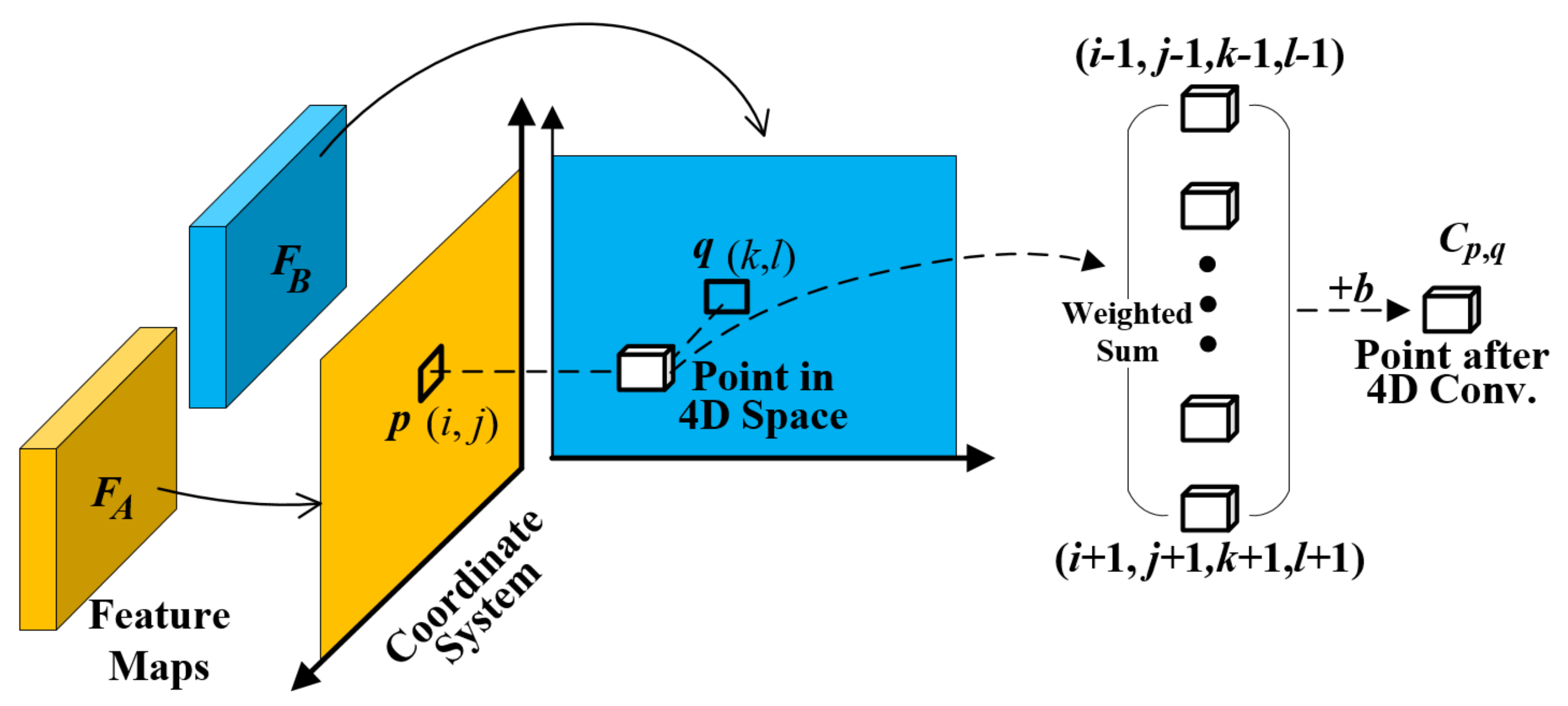
3.3. Four-Dimensional Convolution

The size of the 4D correlation map is ${\left(h\times w\right)}^2$, where $\left(h,w\right)$ represent height and width of the feature map. However, and the correlation number of correct matches is very small, only $\left(h\times w\right)$. This means that the great majority of the information in the correlation map corresponds to matching noise, in other words, the correlation map is easily affected by noise. Since the correlation map serves as the direct cue for semantic matching assignment, its accuracy directly determines the accuracy of the matching. As a result, it is necessary to optimize the correlations to reduce noise interference.

There is a prior knowledge for filter correlations: a correct correlation has a coherent set of supporting correlations in the neighborhood. In other words, the matching continuity in the neighborhood of the image should be equivalently reflected in the correlation continuity in the correlation map. Therefore, we explore neighborhood consensus of the correlation space based on this prior knowledge. Here, we adopt a series of learnable convolution kernels to slide in the correlation space to constrain the contextual consistency, thereby correcting some outlier correlations.

Specifically, since the space of the correlation map is four-dimensional, that is, combining two horizontal dimensions and two vertical dimensions of two feature maps, we use 4D convolution to process the correlation map as shown in Figure 4. It shows the convolution of $C_{i,j,k,l}$’s neighborhood, where $\left(i,j\right)$$\left(k,l\right)$ are the coordinates of points p and q in the feature maps $F_A$ and $F_B$, respectively. Taking the width equal to 3 as an example, the 4D neighbors can be denoted as $C_{i+\Delta i,j+\Delta j,k+\Delta k,l+\Delta l}$, where $-1\le \Delta i,\Delta k,\Delta k,\Delta l\le 1$. Each 4D convolution kernel convolves this neighborhood to learn a specific local structure pattern. Its process can be regarded as a weighted average with a bias:

$$C_{i,j,k,l}=\left(\sum _{\Delta i}\sum _{\Delta j}\sum _{\Delta k}\sum _{\Delta l}{W}_{\Delta i,\Delta j,\Delta k,\Delta l}{C}_{i+\Delta i,j+\Delta j,k+\Delta k,l+\Delta l}\right)+b,$$

(5)

where the weight $W_{\Delta i,\Delta j,\Delta k,\Delta l}$ and the bias b are learnable parameters. Similar to 2D convolution, we use a series of 4D convolutions to capture more complex local structures to obtain more accurate correlations.

3.4. Objective Function

Semantic matching lacks dense ground-truth correspondences, and manual annotation is quite difficult. To train the semantic matching network without dense ground truth, one approach is to use auxiliary labels. For example, the image can be rendered by a known 3D model [21], the matching between images can be converted to the matching between 3D models, and the latter has known matching relationships. However, the final semantic matching accuracy of this method depends on the correctness of auxiliary labels and the accuracy of the conversion process. Another way is to construct training image pairs using a pre-defined geometric transformation (affine/homography) model [40]. As a result, one image can be transformed to another and their correspondences can be calculated since the transformation model are known. However, such synthesized images are still different from real images, that is, the difference between the synthesized image and the original real image is rigid, while there are lots of non-rigid differences between two real images. In contrast, our method directly uses specific labels provided by the semantic matching dataset as the strong supervision signal to train the network, which avoids the potential matching inaccuracy caused by rendering or transforming the image.

Instead of using the foreground-mask correspondences as supervision signals [34], our method uses keypoint labels since they have pixel-level ground-truth matches. This stronger supervision signal can guide the network to estimate the matching field between images. Specifically, a landmark loss is defined, which is the average Euclidean distance between ground-truth keypoint p in the source image and the estimated one $p^{\prime }$ by translating its corresponding target keypoint q to the source with the predicted correspondence:

$$L_{landmark}=\frac{1}{N}\sum _i^N{∥p_i-p_i^{\prime }∥}_2^2,$$

(6)

where N is the number of keypoints. During training, the network can gradually estimate the semantic matching field, where all the estimated keypoints are as close as possible to the real keypoints in space.

In addition, an unsupervised loss named consistency loss is used to assist network training, which works on all points in the image, but its constraint ability is not as strong as the landmark loss. Specifically, consistency loss is defined as the average Euclidean distance between initial point p in the source image and estimated point $p^{″}$ calculated by source-to-target and then target-to-source mappings:

$$L_{consistency}=\frac{1}{N^{\prime }}\sum _i^{N^{\prime }}{∥p_i-p_i^{″}∥}_2^2,$$

(7)

where $N^{\prime }$ is the number of all pixels in the image. We define the overall objective function as

$$L={\lambda }_1{L}_{landmark}+{\lambda }_2{L}_{consistency},$$

(8)

where ${\lambda }_1$ and ${\lambda }_2$ are the coefficients for landmark loss and consistency loss, respectively.

4. Experiments

In this section, we first describe the implementation details of the proposed algorithm (Section 4.1). To analyze the performance of our method, we performed quantitative and qualitative experiments as well as ablation analysis. The quantitative experiment (Section 4.2) compares the matching accuracy of different methods. The qualitative experiment (Section 4.3) evaluates the matching accuracy by analyzing warping quality based on the estimated semantic matching field. The ablation experiment (Section 4.4) compares different variants of the model to verify the effectiveness of each module. Finally, we show the application of semantic matching in label transfer (Section 4.6).

4.1. Implementation Details

We train our network under the PyTorch framework [43] with ResNet-101 [26] as our backbone, since ResNet has a good ability to extract semantics from images. In order to obtain semantic features with segmentation information, we pre-trained a ResNet-101-based fully convolutional network on the COCO2017 dataset [41], which has 20 scenarios. The stride of 4D convolution is set to 1, and its kernel size is set to 5 × 5 × 5 × 5. To ensure that the convolution does not change the size of the correlation map, we set the padding to 2. To train the network for semantic matching, we employ the training set of the PF-PASCAL dataset [9] and resize the training image into 320 × 320.

4.2. Quantitative Results

The PF-PASCAL benchmark [9] is built from the PASCAL VOC 2011 dataset [44] and contains 20 categories and a total of more than 1300 image pairs. These images are annotated with keypoints, which are used for network training and the evaluation of semantic matching performance. The PF-PASCAL dataset is divided into three subsets, namely training set, validation set, and test set. We trained the proposed model on the training set and used the test set to test the matching performance. To verify the domain adaptability of the model, we applied the trained model to the PF-WILLOW dataset [23]. The PF-WILLOW dataset consists of 900 image pairs.

To quantitatively evaluate the semantic matching performance, we use the percentage of correct keypoints (PCK) as the metric. Specifically, we first map the keypoints in the target image to the source image according to estimated semantic correspondences, then calculate the Euclidean distance between the estimated keypoint and the real keypoint in the source image. If the distance is less than $\alpha ·\max \left(h,w\right)$, where h and w are height and width of the image or the bounding box, then the estimated keypoint is considered accurate. The formula of PCK is as follows:

$$\mathrm{PCK}=\frac{1}{N_p}\sum _{\left(p_s,p_t\right)\in \mathcal{P}}\mathbf{1}\left[d\left(p_s,{\mathcal{T}}_{t\to s}\left(p_t\right)\right)\le \alpha ·\max \left(h,w\right)\right],$$

(9)

where $N_p$ is the number of keypoint pairs $\left(p_s,p_t\right)$ on an image pair, and ${\mathcal{T}}_{t\to s}$ is the estimated matching field from the target image to the source image. The larger the PCK value, the more keypoints with correct matching. The final PCK of a benchmark is evaluated by averaging PCKs of all input image pairs.

Table 1. Evaluation results on PF-PASCAL and PF-WILLOW. The best average PCK scores are in bold. The data are sourced from [45] and the running results of source codes.

Methods	PF-PASCAL ($\mathit{\alpha }$ img)			PF-WILLOW ($\mathit{\alpha }$ bbox)
	$\mathbf{\alpha }=\mathbf{0}.\mathbf{05}$	$\mathbf{\alpha }=\mathbf{0}.\mathbf{10}$	$\mathbf{\alpha }=\mathbf{0}.\mathbf{15}$	$\mathbf{\alpha }=\mathbf{0}.\mathbf{05}$	$\mathbf{\alpha }=\mathbf{0}.\mathbf{10}$	$\mathbf{\alpha }=\mathbf{0}.\mathbf{15}$
UCN-ST [8]	0.299	0.556	0.740	0.241	0.540	0.665
SCNet [35]	0.362	0.722	0.820	0.386	0.704	0.853
A2Net [46]	0.428	0.708	0.833	0.363	0.688	0.844
CNNGeo [40]	0.460	0.758	0.884	0.382	0.712	0.858
SFNet [34]	-	0.787	-	-	0.740	-
Weakalign [47]	0.490	0.748	0.840	0.370	0.702	0.799
CAT-FCSS [22]	0.336	0.689	0.792	0.362	0.546	0.692
RTNs [45]	0.552	0.759	0.852	0.413	0.719	0.862
SAOLD [48]	0.528	0.727	0.792	-	-	-
NCNet [31]	0.542	0.789	0.860	0.440	0.727	0.854
Ours	0.555	0.842	0.932	0.454	0.747	0.863

shows the quantitative experimental results. It can be seen that on the PF-PASCAL dataset, our method has a higher PCK than other semantic matching methods, indicating the superior performance of our algorithm. On the PF-WILLOW dataset, our method also obtains higher PCK values than other algorithms.

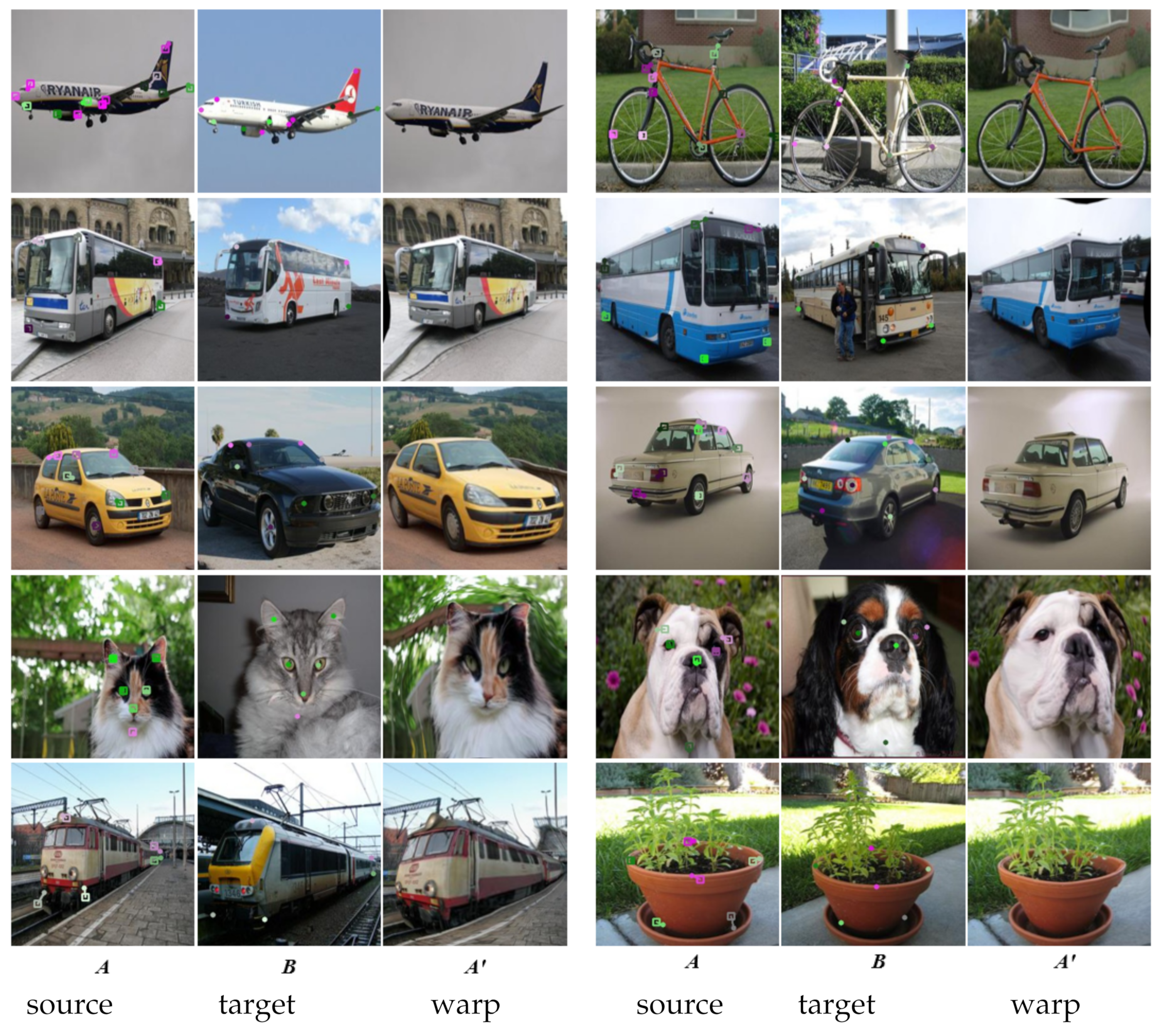
4.3. Qualitative Results

In line with previous works, we used the keypoint-based PCK as the quantitative metric for evaluating semantic matching accuracy, but we still hope to qualitatively evaluate the dense matching performance of our method. Therefore, we warped the image according to the estimated dense semantic matching field and analyzed the matching accuracy of all points according to the warping quality. Specifically, we warped the source image to make it semantically aligned with the target image. Ideally, the warped images and target images should have the same semantic content at the same position on the image. Figure 5 presents some warping examples based on our semantic matching method. It shows that in different scenarios, on the one hand, the object in the warped image is similar to the object in the target image, and on the other hand, the warped images are smooth with less distortion and artifacts. This demonstrates that in addition to the keypoints, the network can also establish good semantic correspondences for other points in the image.

We visualized the keypoint estimation errors as shown by the color line segments in the first and fourth columns of Figure 5. In these source images, the dots represent ground-truth keypoints; the boxes represent the estimated keypoints by translating ground-truth keypoints from target images to the source according to the predicted semantic correspondence. Ideally, the dot and the box should coincide on the image, that is, they should have the same coordinates. However, due to the semantic matching error, there is a spatial deviation between them, as shown by the line segment between the dot and the box. The longer line segment means the greater error of semantic matching. Figure 5 shows that in different scenarios, the spatial deviations between the real and estimated keypoints of our method are small.

4.4. Ablation Study

To verify the effectiveness of each module in the network, namely the 4D convolution and the feature extractor based on semantic segmentation, we designed different algorithm variants shown in

Table 2. Ablation analysis. ✓ indicates that the corresponding component is included, and × indicates that the component has been removed. The best PCK results are in bold.

Semantic Segment	4D Convolution	PF-PASCAL
		$\mathbf{\alpha }=\mathbf{0}.\mathbf{05}$	$\mathbf{\alpha }=\mathbf{0}.\mathbf{10}$	$\mathbf{\alpha }=\mathbf{0}.\mathbf{15}$
×	×	0.306	0.499	0.612
×	✓	0.409	0.740	0.865
✓	✓	0.555	0.842	0.932

, where ✓ means that the module is included, while × indicates that the module is not included. Comparing the first and second rows, PCK is significantly improved after adding 4D convolution. When comparing the second and third rows, PCK is further improved after the semantic segmentation information is added to the feature extractor. It demonstrates that the feature based on semantic segmentation and the 4D convolution both have positive effects on semantic matching.

We visualized the keypoint estimation as shown in Figure 6 to analyze the importance of each module from a qualitative perspective. The second to fourth columns are obtained by the variant algorithms of the first to third rows of Table 2, respectively. The colored line segments in the images connect real keypoints and estimated keypoints. They indicate semantic matching errors since the keypoint estimation is based on keypoint transferring according to semantic matching. The longer the line segment, the greater the error. Figure 6 shows that by adding the 4D convolution and the information of semantic segmentation, the colored line segments gradually become shorter, demonstrating the gradual reduction of keypoint estimation errors and the improvement of semantic matching accuracy.

4.5. Limitation

If the object in the image is occluded, there might be incorrect semantic matching in the occluded area. Figure 7 is a erroneous matching example due to occlusion, where the car is partially occluded by a person (see the target image). Since it lacks the semantic information of the car in occluded regions, the semantic matching cannot be estimated correctly. Based on such incorrect semantic correspondences, the warped image cannot be guaranteed to be semantically aligned with the target image (see the blue boxes).

4.6. Application

There are many applications of semantic matching. Here, we give an example of its application in label transfer. Manual labeling is very time-consuming work; however, if there are some known labels in the images, transferring them to other images through algorithms can greatly reduce labor costs. For example, we can transfer the foreground mask across images based on semantic consistency as shown in Figure 8. The first and third columns are semantically similar images. According to the estimated pixel-to-pixel semantic matches between them, the known foreground masks of one image are easily transferred to another one. The last column shows transfer results.

5. Conclusions

We have proposed a convolutional neural network to achieve dense semantic matching. To remove some potential matching errors, we combined the feature extraction based on semantic segmentation and the neighborhood consensus exploration based on 4D convolution. Quantitative and quantitative experiments demonstrate that our method has higher semantic matching accuracy than other methods, and can establish correct and smooth semantic matching for all points (not only keypoints) in the image. The ablation experiment shows the benefits of semantic segmentation information and 4D convolution on matching accuracy. It indicates that the proposed consideration of semantic segmentation information can enrich the semantic representation at the feature level, thereby reducing mismatches. We have presented the application of semantic matching in label transfer.

There are two future research directions. One is to study the estimation of dense semantic matching between two images with occlusion or truncation or different perspectives. In these cases, a point may need to combine neighborhood features and matches, or it may need to consider the global representation. Another direction is to study potential applications, such as exemplar-based image translation and enhancement. These applications need to establish semantic matching between the template and the image, so that the image can obtain information from the same semantic region on the template.

References

1. Scharstein, D.; Szeliski, R. A taxonomy and evaluation of dense two-frame stereo correspondence algorithms. Int. J. Comput. Vis. 2002, 47, 7–42. [Google Scholar] [CrossRef]
2. Liu, H.; Wang, R.; Xia, Y.; Zhang, X. Improved Cost Computation and Adaptive Shape Guided Filter for Local Stereo Matching of Low Texture Stereo Images. Appl. Sci. 2020, 10, 1869. [Google Scholar] [CrossRef] [Green Version]
3. Xu, H.; Chen, X.; Liang, H.; Ren, S.; Wang, Y.; Cai, H. Crosspatch-based rolling label expansion for dense stereo matching. IEEE Access 2020, 8, 63470–63481. [Google Scholar] [CrossRef]
4. Brox, T.; Bruhn, A.; Papenberg, N.; Weickert, J. High accuracy optical flow estimation based on a theory for warping. In Proceedings of the European Conference on Computer Vision, Prague, Szech Republic, 11–14 May 2004; Springer: Berlin/Heidelberg, Germany, 2004; pp. 25–36. [Google Scholar]
5. Horn, B.K.; Schunck, B.G. Determining optical flow. Artif. Intell. 1981, 17, 185–203. [Google Scholar] [CrossRef] [Green Version]
6. Long, J.L.; Zhang, N.; Darrell, T. Do convnets learn correspondence? In Proceedings of the Advances in Neural Information Processing Systems, Montreal, QC, Canada, 8–13 December 2014; pp. 1601–1609. [Google Scholar]
7. Kanazawa, A.; Jacobs, D.W.; Chandraker, M. Warpnet: Weakly supervised matching for single-view reconstruction. In Proceedings of the IEEE Conference on Computer Vision and Pattern Recognition, Las Vegas, NV, USA, 27–30 June 2016; pp. 3253–3261. [Google Scholar]
8. Choy, C.B.; Gwak, J.; Savarese, S.; Chandraker, M. Universal correspondence network. arXiv 2016, arXiv:1606.03558. [Google Scholar]
9. Ham, B.; Cho, M.; Schmid, C.; Ponce, J. Proposal flow: Semantic correspondences from object proposals. IEEE Trans. Pattern Anal. Mach. Intell. 2017, 40, 1711–1725. [Google Scholar] [CrossRef] [PubMed] [Green Version]
10. Jeon, S.; Kim, S.; Min, D.; Sohn, K. Parn: Pyramidal affine regression networks for dense semantic correspondence. In Proceedings of the European Conference on Computer Vision (ECCV), Munich, Germany, 8–14 September 2018; pp. 351–366. [Google Scholar]
11. Liao, J.; Yao, Y.; Yuan, L.; Hua, G.; Kang, S.B. Visual attribute transfer through deep image analogy. arXiv 2017, arXiv:1705.01088. [Google Scholar] [CrossRef] [Green Version]
12. Liu, C.; Yuen, J.; Torralba, A. Sift flow: Dense correspondence across scenes and its applications. IEEE Trans. Pattern Anal. Mach. Intell. 2010, 33, 978–994. [Google Scholar] [CrossRef] [PubMed] [Green Version]
13. Aberman, K.; Liao, J.; Shi, M.; Lischinski, D.; Chen, B.; Cohen-Or, D. Neural best-buddies: Sparse cross-domain correspondence. ACM Trans. Graph. (TOG) 2018, 37, 1–14. [Google Scholar] [CrossRef] [Green Version]
14. He, M.; Chen, D.; Liao, J.; Sander, P.V.; Yuan, L. Deep exemplar-based colorization. ACM Trans. Graph. (TOG) 2018, 37, 1–16. [Google Scholar] [CrossRef] [Green Version]
15. Bansal, A.; Sheikh, Y.; Ramanan, D. Pixelnn: Example-based image synthesis. arXiv 2017, arXiv:1708.05349. [Google Scholar]
16. Zhang, P.; Zhang, B.; Chen, D.; Yuan, L.; Wen, F. Cross-domain correspondence learning for exemplar-based image translation. In Proceedings of the IEEE/CVF Conference on Computer Vision and Pattern Recognition, Seattle, WA, USA, 13–19 June 2020; pp. 5143–5153. [Google Scholar]
17. Zhang, Z.; Wang, Z.; Lin, Z.; Qi, H. Image super-resolution by neural texture transfer. In Proceedings of the IEEE/CVF Conference on Computer Vision and Pattern Recognition, Long Beach, CA, USA, 15–20 June 2019; pp. 7982–7991. [Google Scholar]
18. Lowe, D.G. Distinctive image features from scale-invariant keypoints. Int. J. Comput. Vis. 2004, 60, 91–110. [Google Scholar] [CrossRef]
19. Tola, E.; Lepetit, V.; Fua, P. Daisy: An efficient dense descriptor applied to wide-baseline stereo. IEEE Trans. Pattern Anal. Mach. Intell. 2009, 32, 815–830. [Google Scholar] [CrossRef] [PubMed] [Green Version]
20. Dalal, N.; Triggs, B. Histograms of oriented gradients for human detection. In Proceedings of the 2005 IEEE Computer Society Conference on Computer Vision and Pattern Recognition (CVPR’05), San Diego, CA, USA, 20–26 June 2005; Volume 1, pp. 886–893. [Google Scholar]
21. Zhou, T.; Krahenbuhl, P.; Aubry, M.; Huang, Q.; Efros, A.A. Learning dense correspondence via 3d-guided cycle consistency. In Proceedings of the IEEE Conference on Computer Vision and Pattern Recognition, Las Vegas, NV, USA, 27–30 June 2016; pp. 117–126. [Google Scholar]
22. Kim, S.; Min, D.; Ham, B.; Jeon, S.; Lin, S.; Sohn, K. Fcss: Fully convolutional self-similarity for dense semantic correspondence. In Proceedings of the IEEE Conference on Computer Vision and Pattern Recognition, Honolulu, HI, USA, 21–27 July 2017; pp. 6560–6569. [Google Scholar]
23. Ham, B.; Cho, M.; Schmid, C.; Ponce, J. Proposal flow. In Proceedings of the IEEE Conference on Computer Vision and Pattern Recognition, Las Vegas, NV, USA, 27–30 June 2016; pp. 3475–3484. [Google Scholar]
24. Russakovsky, O.; Deng, J.; Su, H.; Krause, J.; Satheesh, S.; Ma, S.; Huang, Z.; Karpathy, A.; Khosla, A.; Bernstein, M.; et al. Imagenet large scale visual recognition challenge. Int. J. Comput. Vis. 2015, 115, 211–252. [Google Scholar] [CrossRef] [Green Version]
25. Simonyan, K.; Zisserman, A. Very deep convolutional networks for large-scale image recognition. arXiv 2014, arXiv:1409.1556. [Google Scholar]
26. He, K.; Zhang, X.; Ren, S.; Sun, J. Deep residual learning for image recognition. In Proceedings of the IEEE Conference on Computer Vision and Pattern Recognition, Las Vegas, NV, USA, 27–30 June 2016; pp. 770–778. [Google Scholar]
27. Schaffalitzky, F.; Zisserman, A. Automated scene matching in movies. In Proceedings of the International Conference on Image and Video Retrieval, London, UK, 18–19 July 2002; Springer: Berlin/Heidelberg, Germany, 2002; pp. 186–197. [Google Scholar]
28. Sivic, J.; Zisserman, A. Video Google: A text retrieval approach to object matching in videos. In Proceedings of the IEEE International Conference on Computer Vision, Madison, WI, USA, 18–20 June 2003; IEEE Computer Society: Washington, DC, USA; Volume 3, p. 1470. [Google Scholar]
29. Sattler, T.; Leibe, B.; Kobbelt, L. SCRAMSAC: Improving RANSAC’s efficiency with a spatial consistency filter. In Proceedings of the 2009 IEEE 12th International Conference on Computer Vision, Kyoto, Japan, 29 September–2 October 2009; IEEE: Piscataway, NJ, USA, 2009; pp. 2090–2097. [Google Scholar]
30. Bian, J.; Lin, W.Y.; Matsushita, Y.; Yeung, S.K.; Nguyen, T.D.; Cheng, M.M. Gms: Grid-based motion statistics for fast, ultra-robust feature correspondence. In Proceedings of the IEEE Conference on Computer Vision and Pattern Recognition, Honolulu, HI, USA, 21–26 July 2017; pp. 4181–4190. [Google Scholar]
31. Rocco, I.; Cimpoi, M.; Arandjelović, R.; Torii, A.; Pajdla, T.; Sivic, J. Neighbourhood consensus networks. arXiv 2018, arXiv:1810.10510. [Google Scholar]
32. Novotny, D.; Larlus, D.; Vedaldi, A. Anchornet: A weakly supervised network to learn geometry-sensitive features for semantic matching. In Proceedings of the IEEE Conference on Computer Vision and Pattern Recognition, Honolulu, HI, USA, 21–26 July 2017; pp. 5277–5286. [Google Scholar]
33. Huang, S.; Wang, Q.; Zhang, S.; Yan, S.; He, X. Dynamic context correspondence network for semantic alignment. In Proceedings of the IEEE/CVF International Conference on Computer Vision, Seoul, Korea, 27–28 October 2019; pp. 2010–2019. [Google Scholar]
34. Lee, J.; Kim, D.; Ponce, J.; Ham, B. Sfnet: Learning object-aware semantic correspondence. In Proceedings of the IEEE/CVF Conference on Computer Vision and Pattern Recognition, Long Beach, CA, USA, 15–20 June 2019; pp. 2278–2287. [Google Scholar]
35. Han, K.; Rezende, R.S.; Ham, B.; Wong, K.Y.K.; Cho, M.; Schmid, C.; Ponce, J. Scnet: Learning semantic correspondence. In Proceedings of the IEEE International Conference on Computer Vision, Venice, Italy, 22–29 October 2017; pp. 1831–1840. [Google Scholar]
36. Shechtman, E.; Irani, M. Matching local self-similarities across images and videos. In Proceedings of the 2007 IEEE Conference on Computer Vision and Pattern Recognition, Minneapolis, MN, USA, 18–23 June 2007; IEEE: Piscataway, NJ, USA, 2007; pp. 1–8. [Google Scholar]
37. Kim, S.; Min, D.; Lin, S.; Sohn, K. Deep self-correlation descriptor for dense cross-modal correspondence. In Proceedings of the European Conference on Computer Vision, Amsterdam, The Netherlands, 8–16 October 2016; Springer: Berlin/Heidelberg, Germany, 2016; pp. 679–695. [Google Scholar]
38. Kim, S.; Min, D.; Ham, B.; Ryu, S.; Do, M.N.; Sohn, K. DASC: Dense adaptive self-correlation descriptor for multi-modal and multi-spectral correspondence. In Proceedings of the IEEE Conference on Computer Vision and Pattern Recognition, Boston, MA, USA, 7–12 June 2015; pp. 2103–2112. [Google Scholar]
39. Kim, S.; Min, D.; Lin, S.; Sohn, K. Dctm: Discrete-continuous transformation matching for semantic flow. In Proceedings of the IEEE International Conference on Computer Vision, Venice, Italy, 22–29 October 2017; pp. 4529–4538. [Google Scholar]
40. Rocco, I.; Arandjelovic, R.; Sivic, J. Convolutional neural network architecture for geometric matching. In Proceedings of the IEEE Conference on Computer Vision and Pattern Recognition, Honolulu, HI, USA, 21–26 July 2017; pp. 6148–6157. [Google Scholar]
41. Lin, T.Y.; Maire, M.; Belongie, S.; Hays, J.; Perona, P.; Ramanan, D.; Dollár, P.; Zitnick, C.L. Microsoft coco: Common objects in context. In Proceedings of the European Conference on Computer Vision, Zurich, Switzerland, 6–12 September 2014; Springer: Berlin/Heidelberg, Germany, 2014; pp. 740–755. [Google Scholar]
42. Everingham, M.; Van Gool, L.; Williams, C.K.I.; Winn, J.; Zisserman, A. The PASCAL Visual Object Classes Challenge 2012 (VOC2012) Results. Available online: http://www.pascal-network.org/challenges/VOC/voc2012/workshop/index.html (accessed on 10 January 2021).
43. Paszke, A.; Gross, S.; Chintala, S.; Chanan, G.; Yang, E.; DeVito, Z.; Lin, Z.; Desmaison, A.; Antiga, L.; Lerer, A. Automatic Differentiation in Pytorch. 2017. Available online: http://https://pytorch.org/ (accessed on 12 December 2020).
44. Everingham, M.; Van Gool, L.; Williams, C.K.I.; Winn, J.; Zisserman, A. The PASCAL Visual Object Classes Challenge 2011 (VOC2011) Results. Available online: http://www.pascal-network.org/challenges/VOC/voc2011/workshop/index.html (accessed on 20 January 2021).
45. Kim, S.; Lin, S.; Jeon, S.R.; Min, D.; Sohn, K. Recurrent transformer networks for semantic correspondence. Adv. Neural Inf. Process. Syst. 2018, 31, 6126–6136. [Google Scholar]
46. Seo, P.H.; Lee, J.; Jung, D.; Han, B.; Cho, M. Attentive semantic alignment with offset-aware correlation kernels. In Proceedings of the European Conference on Computer Vision (ECCV), Munich, Germany, 8–14 September 2018; pp. 349–364. [Google Scholar]
47. Rocco, I.; Arandjelović, R.; Sivic, J. End-to-end weakly-supervised semantic alignment. In Proceedings of the IEEE Conference on Computer Vision and Pattern Recognition, Salt Lake City, UT, USA, 18–22 June 2018; pp. 6917–6925. [Google Scholar]
48. Jeon, S.; Min, D.; Kim, S.; Sohn, K. Joint learning of semantic alignment and object landmark detection. In Proceedings of the IEEE/CVF International Conference on Computer Vision, Seoul, Korea, 27 October–2 November 2019; pp. 7294–7303. [Google Scholar]
Figure 1. Semantic matching examples, in which colored line segments represent some semantic matching pairs.
Applsci 11 04648 g001
Figure 2. The pipeline of the proposed method. Two images A , B are fed into the feature extractor, and then the features in different layers are used to calculate the correlation maps C 1 , C 2 , which will be combined and then go through 4D convolution, finally guiding the semantic matching assignment.
Applsci 11 04648 g002
Figure 3. The construction of the feature extractor. It is divided into two steps. The first step is (a): pre-training the semantic segmentation network, which inputs images, calculates a series of feature maps and heat maps, and finally outputs semantic segmentation results. The second step is (b): feature adaptation, where part of the semantic segmentation features (the orange block) are fine-tuned to be semantic matching features Φ 3 , Φ 4 by convolution operation.
Applsci 11 04648 g003
Figure 4. Four-dimensional convolution. The feature maps F A and F B are extracted by a fully convolutional feature extractor. All pairs of individual matches p and q are represented in the 4D space of matches i , j , k , l , and the matching score is stored in the correlation C p , q . The 4D convolution can be regarded as the weighted sum of correlations within the 4D neighborhood.
Applsci 11 04648 g004
Figure 5. Image warping and keypoint estimation visualization. The warped images are semantically aligned with the target images. The color line segments (in columns 1 and 4) depict semantic matching errors, where the dots represent ground-truth keypoints, while the boxes represent the estimated keypoints by keypoint transferring from the target image to the source based on the predicted semantic matching.
Applsci 11 04648 g005
Figure 6. Keypoint estimation visualization. A represents the source image, and B 1 , B 2 , and B 3 are target images. The dots in these images are the ground-truth keypoints, the boxes are the transferring results of keypoints from source to target images according to semantic matching. The color line segments are the keypoint estimation errors. B 1 , B 2 , and B 3 correspond to different variant algorithms from the first row to the third row of Table 2.
Applsci 11 04648 g006
Figure 7. Erroneous semantic correspondence due to occlusion. The orange solid line is the estimated match by our algorithm; the dashed line is the ground-truth match. The right image is a warping result according to dense semantic matching between source and target images, which should be semantically aligned with the target theoretically. The blue boxes mark the areas with mismatches and bad warping.
Applsci 11 04648 g007
Figure 8. Semantic label transfer. The second column shows the real foreground masks of A. The last column is the estimated mask of B, which is obtained by warping A’s mask according to the dense semantic matching between A and B.
Applsci 11 04648 g008