
Fuzzy Graph Learning Regularized Sparse Filtering for Visual Domain Adaptation


Abstract
1. Introduction
- We propose a novel solution for UDA problems, which is able to learn both discriminative and domain-shared representations simultaneously. Extensive experiments on several real-world datasets demonstrate its superiority to existing works.
- Different from previous hard-labeling methods, we design a fuzzy graph regularization based on soft-labeling. Specifically, it attempts to describe cross-domain affinity by means of probability matrix.
- In order to deal with the problem of representation shrinkage, we combine the proposed fuzzy graph regularization with unsupervised sparse filtering, so that the two objective will be antagonistic and converge to a compromise.
2. Related Works
2.1. Domain Adaptation
2.1.1. Pseudo Label without Selection
2.1.2. Pseudo Label with Selection
2.2. Sparse Filtering
- Population Sparsity. Each example should be represented by only a few active features. Ideally, a sample should be a vector which contains lots of zeros and few non-zero values.
- Lifetime Sparsity. Good features should be distinguishable, therefore, a feature is only allowed to be activated in few samples. On the contrary, if a feature is activated by all the samples, we cannot classify samples according to this feature, so it is not a good feature.
- High Dispersal. It requires each feature to have similar statistical properties across all samples, which seems to be useless. The authors indicate that this can prevent feature degradation, such as similar features across samples.
3. Methodology
3.1. Problem Definition and Notations
3.2. Fuzzy Graph Learning for Domain Alignment
| Algorithm 1: Cross-domain affinity graph () construction. |
 |
3.3. Sparse Filtering for Discriminative Feature Learning
3.4. Optimization
3.4.1. Gradient of
3.4.2. Gradient of
3.4.3. Gradient of
3.4.4. Unified Optimization Based on Gradient Descent
| Algorithm 2: Optimization of the proposed method. |
 |
4. Experiments
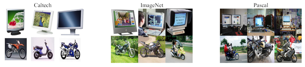
4.1. Datasets
4.2. Experimental Setting
- Nearest Neighbor(NN) [23]. NN is served as a baseline model to check whether the learned representations really work for DA problems.
- Joint Distribution Alignment(JDA) [14]. JDA [Long et al. ICCV2013] adopts pseudo labels to align the conditional distributions of two domains.
- Correlation Alignment(CORAL) [7]. CORAL [Sun et al. AAAI2016] obtains transferable representations by aligning the second-order statistics of distributions.
- Confidence-Aware Pseudo Label Selection(CAPLS) [17]. CAPLS [Wang et al. IJCNN2019] uses a selective pseudo labeling procedure to obtain more reliable labels.
- Modified A-distance Sparse Filtering(MASF) [24]. MASF [Han et al. Pattern Recognit.2020] employs an L2 constraint combining sparse filtering to learn both domain-shared and discriminative representations.
- Selective Pseudo Labeling(SPL) [18]. SPL [Wang et al. AAAI2020] is also a selective pseudo labeling strategy based on structured prediction.
4.3. Results
- FGLSF vs. NN. According to the results, FGLSF is significantly better than NN. NN cannot handle the domain discrepancy, thus results in unsatisfying performance. On the other hand, it indicates that our method is able to learn transferable representations.
- FGLSF vs. CORAL, JDA. FGLSF is superior to CORAL and JDA. This two methods are classical distribution matching works, but they have limited considerations on the discrimination of learned representations.
- FGLSF vs. MASF. MASF is another framework based on sparse filtering, which adopts a modified distance for domain alignment. Compared to our method, it cannot deal with the problem of conditional distribution matching.
- FGLSF vs. CAPLS, SPL. Objectively speaking, our method FGLSF has comparable performance when compared state-of-the-art selective hard labeling method, only a 0.3% improvement is gained. It shows that the proposed fuzzy graph regularization is also valid for alleviating the negative effects caused by wrong labeling.
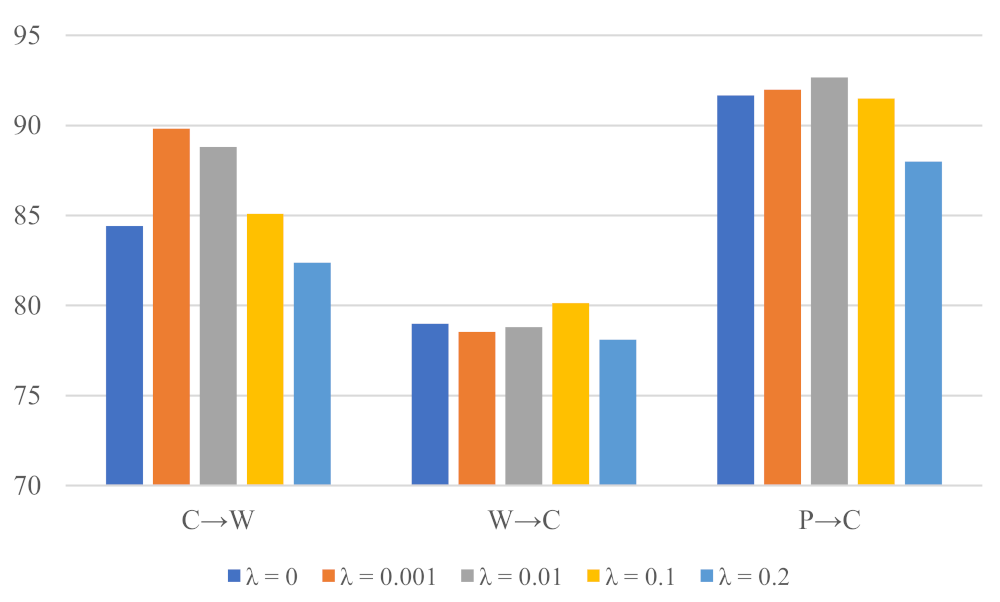
4.4. Parameter Sensitivity Analysis
5. Discussion
5.1. Does Iterative Learning Help Improve the Model?
5.2. Fuzzy Labeling versus Selective Hard Labeling
6. Conclusions
Author Contributions
Funding
Conflicts of Interest
References
- Saenko, K.; Kulis, B.; Fritz, M.; Darrell, T. Adapting visual category models to new domains. In European Conference on Computer Vision; Springer: Berlin/Heidelberg, Germany, 2010; pp. 213–226. [Google Scholar]
- Patel, V.M.; Gopalan, R.; Li, R.; Chellappa, R. Visual Domain Adaptation: A survey of recent advances. IEEE Signal Process. Mag. 2015, 32, 53–69. [Google Scholar] [CrossRef]
- Li, X.; Grandvalet, Y.; Davoine, F.; Cheng, J.; Cui, Y.; Zhang, H.; Belongie, S.; Tsai, Y.; Yang, M. Transfer learning in computer vision tasks: Remember where you come from. Image Vis. Comput. 2020, 93, 103853. [Google Scholar] [CrossRef]
- Pan, S.J.; Yang, Q. A Survey on Transfer Learning. IEEE Trans. Knowl. Data Eng. 2010, 22, 1345–1359. [Google Scholar] [CrossRef]
- Wang, M.; Deng, W. Deep visual domain adaptation: A survey. Neurocomputing 2018, 312, 135–153. [Google Scholar] [CrossRef]
- Smola, A.J.; Gretton, A.; Song, L.; Scholkopf, B. A Hilbert Space Embedding for Distributions. In Algorithmic Learning Theory; Springer: Berlin/Heidelberg, Germany, 2007; pp. 13–31. [Google Scholar]
- Sun, B.; Feng, J.; Saenko, K. Return of frustratingly easy domain adaptation. In Proceedings of the National Conference on Artificial Intelligence, Phoenix, AZ, USA, 2–9 February 2016; pp. 2058–2065. [Google Scholar]
- Pan, S.J.; Tsang, I.W.; Kwok, J.T.; Yang, Q. Domain Adaptation via Transfer Component Analysis. IEEE Trans. Neural Netw. Learn. Syst. 2011, 22, 199–210. [Google Scholar] [CrossRef] [PubMed]
- Zhang, W.; Ouyang, W.; Li, W.; Xu, D. Collaborative and Adversarial Network for Unsupervised Domain Adaptation. In Proceedings of the Computer Vsion and Pattern Recognition, Salt Lake City, UT, USA, 18–22 June 2018; pp. 3801–3809. [Google Scholar]
- Tzeng, E.; Hoffman, J.; Saenko, K.; Darrell, T. Adversarial Discriminative Domain Adaptation. In Proceedings of the Computer Vsion and Pattern Recognition, Honolulu, HI, USA, 21–26 July 2017; pp. 2962–2971. [Google Scholar]
- Ganin, Y.; Lempitsky, V. Unsupervised Domain Adaptation by Backpropagation. In Proceedings of the International Conference on Machine Learning, Lille, France, 6–11 July 2015; pp. 1180–1189. [Google Scholar]
- Yan, H.; Ding, Y.; Li, P.; Wang, Q.; Xu, Y.; Zuo, W. Mind the Class Weight Bias: Weighted Maximum Mean Discrepancy for Unsupervised Domain Adaptation. In Proceedings of the Computer Vsion and Pattern Recognition, Honolulu, HI, USA, 21–26 July 2017; pp. 945–954. [Google Scholar]
- Ngiam, J.; Chen, Z.; Bhaskar, S.A.; Koh, P.W.; Ng, A.Y. Sparse Filtering. In Proceedings of the Neural Information Processing Systems, Granada, Spain, 12–15 December 2011; pp. 1125–1133. [Google Scholar]
- Long, M.; Wang, J.; Ding, G.; Sun, J.; Yu, P.S. Transfer Feature Learning with Joint Distribution Adaptation. In Proceedings of the International Conference on Computer Vision, Sydney, Australia, 1–8 December 2013; pp. 2200–2207. [Google Scholar]
- He, X.; Niyogi, P. Locality Preserving Projections. In Proceedings of the Neural Information Processing Systems, Vancouver, BC, Canada, 8–13 December 2003; pp. 153–160. [Google Scholar]
- Sanodiya, R.K.; Mathew, J. A novel unsupervised Globality-Locality Preserving Projections in transfer learning. Image Vis. Comput. 2019, 90, 103802. [Google Scholar] [CrossRef]
- Wang, Q.; Bu, P.; Breckon, T.P. Unifying Unsupervised Domain Adaptation and Zero-Shot Visual Recognition. In Proceedings of the International Joint Conference on Neural Network, Budapest, Hungary, 14–19 July 2019; pp. 1–8. [Google Scholar]
- Wang, Q.; Breckon, T.P. Unsupervised Domain Adaptation via Structured Prediction Based Selective Pseudo-Labeling. In Proceedings of the National Conference on Artificial Intelligence, New York, NY, USA, 7–12 February 2020; pp. 1–10. [Google Scholar]
- CaltechAUTHORS. Caltech-256 Object Category Dataset; Technical Report. Pasadena, CA, USA, 2007. Available online: http://www.vision.caltech.edu/Image_Datasets/Caltech256 (accessed on 14 May 2021).
- Deng, J.; Dong, W.; Socher, R.; Li, L.; Li, K.; Feifei, L. ImageNet: A large-scale hierarchical image database. In Proceedings of the Computer Vsion and Pattern Recognition, Miami, FL, USA, 20–25 June 2009; pp. 248–255. [Google Scholar]
- Everingham, M.; Van Gool, L.; Williams, C.K.I.; Winn, J.; Zisserman, A. The PASCAL Visual Object Classes Challenge 2007 (VOC2007) Results. Available online: http://www.pascal-network.org/challenges/VOC/voc2007/workshop/index.html (accessed on 14 May 2021).
- Gong, B.; Shi, Y.; Sha, F.; Grauman, K. Geodesic flow kernel for unsupervised domain adaptation. In Proceedings of the Computer Vsion and Pattern Recognition, Providence, RI, USA, 16–21 June 2012; pp. 2066–2073. [Google Scholar]
- Cover, T.M.; Hart, P.E. Nearest neighbor pattern classification. IEEE Trans. Inf. Theory 1967, 13, 21–27. [Google Scholar] [CrossRef]
- Han, C.; Lei, Y.; Xie, Y.; Zhou, D.; Gong, M. Visual Domain Adaptation Based on Modified A Distance and Sparse Filtering. Pattern Recognit. 2020, 104, 107254. [Google Scholar] [CrossRef]


| Notations | Description |
|---|---|
| source/target domain | |
| original source/target domain data | |
| source/target domain label | |
| number of source/target samples | |
| original/transformed feature dimension | |
| source/target features | |
| mapping function, | |
| W | the transformation matrix to be solved |
| objective function for fuzzy graph learning | |
| objective function for sparse filtering | |
| the balance factors between two objectives |
| No. | Task | NN | JDA | CORAL | CAPLS | MASF | SPL | JAN | DAN | FGLSF |
|---|---|---|---|---|---|---|---|---|---|---|
| 1 | C→ A | 85.69 | 89.77 | 92.00 | 90.90 | 90.81 | 92.80 | 91.90 | 92.00 | 93.32 |
| 2 | C→ W | 66.10 | 83.73 | 80.00 | 88.83 | 87.46 | 85.08 | 85.40 | 90.60 | 84.75 |
| 3 | C→ D | 74.52 | 86.62 | 84.70 | 90.08 | 89.81 | 91.72 | 88.80 | 89.30 | 87.90 |
| 4 | A→ C | 70.35 | 82.28 | 83.20 | 80.66 | 87.36 | 81.39 | 85.00 | 84.10 | 85.31 |
| 5 | A→ W | 57.29 | 78.64 | 74.60 | 80.69 | 81.02 | 84.07 | 86.10 | 91.80 | 88.14 |
| 6 | A→ D | 64.97 | 80.25 | 84.10 | 89.45 | 86.62 | 90.45 | 89.00 | 91.70 | 87.26 |
| 7 | W→ C | 60.37 | 83.53 | 75.50 | 86.62 | 85.04 | 74.00 | 78.00 | 81.20 | 74.27 |
| 8 | W→ A | 62.53 | 90.19 | 81.20 | 91.38 | 91.34 | 91.96 | 84.90 | 92.10 | 89.25 |
| 9 | W→ D | 98.73 | 100.00 | 100.00 | 100.00 | 99.36 | 100.00 | 100.00 | 100.00 | 97.45 |
| 10 | D→ C | 52.09 | 85.13 | 76.80 | 88.05 | 85.75 | 88.51 | 81.10 | 80.30 | 83.35 |
| 11 | D→ A | 62.73 | 91.44 | 85.50 | 92.32 | 90.40 | 93.32 | 89.50 | 90.00 | 91.75 |
| 12 | D→ W | 89.15 | 98.98 | 99.30 | 98.66 | 98.98 | 100.00 | 98.20 | 98.50 | 95.59 |
| 13 | C→ I | 85.16 | 92.00 | 83.00 | 91.00 | 89.83 | 90.83 | 89.50 | 89.50 | 94.00 |
| 14 | C→ P | 69.16 | 75.50 | 71.50 | 77.33 | 72.83 | 78.17 | 74.20 | 75.80 | 79.70 |
| 15 | I→ C | 91.16 | 92.33 | 88.66 | 94.17 | 93.17 | 94.33 | 94.70 | 94.20 | 97.00 |
| 16 | I→ P | 73.16 | 77.00 | 73.66 | 75.80 | 76.83 | 77.50 | 76.80 | 78.20 | 80.71 |
| 17 | P→ C | 81.33 | 83.83 | 72.50 | 90.67 | 85.33 | 91.33 | 91.70 | 89.20 | 95.50 |
| 18 | P→ I | 74.50 | 79.16 | 72.33 | 85.00 | 80.83 | 85.83 | 88.00 | 87.50 | 93.00 |
| 19 | AVG | 73.28 | 86.13 | 82.14 | 88.42 | 87.38 | 88.40 | 87.38 | 88.66 | 88.79 |
Publisher’s Note: MDPI stays neutral with regard to jurisdictional claims in published maps and institutional affiliations. |
© 2021 by the authors. Licensee MDPI, Basel, Switzerland. This article is an open access article distributed under the terms and conditions of the Creative Commons Attribution (CC BY) license (https://creativecommons.org/licenses/by/4.0/).
Share and Cite
Min, L.; Zhou, D.; Li, X.; Lv, Q.; Zhi, Y. Fuzzy Graph Learning Regularized Sparse Filtering for Visual Domain Adaptation. Appl. Sci. 2021, 11, 4503. https://doi.org/10.3390/app11104503
Min L, Zhou D, Li X, Lv Q, Zhi Y. Fuzzy Graph Learning Regularized Sparse Filtering for Visual Domain Adaptation. Applied Sciences. 2021; 11(10):4503. https://doi.org/10.3390/app11104503
Chicago/Turabian StyleMin, Lingtong, Deyun Zhou, Xiaoyang Li, Qinyi Lv, and Yuanjie Zhi. 2021. "Fuzzy Graph Learning Regularized Sparse Filtering for Visual Domain Adaptation" Applied Sciences 11, no. 10: 4503. https://doi.org/10.3390/app11104503
APA StyleMin, L., Zhou, D., Li, X., Lv, Q., & Zhi, Y. (2021). Fuzzy Graph Learning Regularized Sparse Filtering for Visual Domain Adaptation. Applied Sciences, 11(10), 4503. https://doi.org/10.3390/app11104503