Article

Estimation of Grey-Box Dynamic Model of 2-DOF Pneumatic Actuator Robotic Arm Using Gravity Tests

by
Monika Trojanová
1,
Tomáš Čakurda
1,
Alexander Hošovský
1 and
Tibor Krenický
2,*
1
Department of Industrial Engineering and Informatics, Faculty of Manufacturing Technologies with a Seat in Prešov, Technical University of Košice, Bayerova 1, 080 01 Prešov, Slovakia
2
Department of Technical Systems Design and Monitoring, Faculty of Manufacturing Technologies with a Seat in Prešov, Technical University of Košice, Štúrova 31, 080 01 Prešov, Slovakia
*
Author to whom correspondence should be addressed.
Appl. Sci. 2021, 11(10), 4490; https://doi.org/10.3390/app11104490
Submission received: 23 April 2021 / Revised: 10 May 2021 / Accepted: 12 May 2021 / Published: 14 May 2021

Abstract

:
This article describes the dynamics of a manipulator with two degrees of freedom, while the dynamic model of the manipulator’s arm is derived using Lagrangian formalism, which considers the difference between the kinetic and potential energy of the system. The compiled dynamic model was implemented in Matlab, taking into account the physical parameters of the manipulator and friction term. Physical parameters were exported from the 3D CAD model. A scheme (model) was compiled in the Simulink, which was used for the subsequent validation process. The outputs of the validations were compared with measured data of joint angles from the system (expected condition) obtained by using gravity tests. For obtaining better results were parameters of the model optimizing by using the Trust Region Algorithm for Nonlinear Least Squares optimization method. Therefore, the aim of the research described in the article is the comparison of the model with the parameters that come from CAD and its improvement by estimating the parameters based on gravitational measurements. The model with estimated parameters achieved an improvement in the results of the Normal Root Mean Square Error compared to the model with CAD parameters. For link 1 was an improvement from 28.49% to 67.93% depending on the initial joint angle, and for link 2, from 63.84% to 66.46%.

1. Introduction and Related Works

Robotics has been an area of research that has attracted the attention of scientists around the world for many decades, but in recent years has enjoyed enormous interest, especially in the safe interaction between humans and robots [1]. The robotic system may be assigned tasks that a person cannot perform in some respects, e.g., if the operations are physically demanding for a person, or if the activity requires high accuracy of movement, or last but not least, the operating and working conditions are not suitable for human work in the vicinity of such a mechanism. All these facts give researchers from different fields many actuations to progress in the research and development of robots and manipulators, whether in the process of designing [2,3], production or the actual application of robots [4,5,6,7]. Ref. [4] describes the application of robots, and thus, in particular, the topic of self-employed robots so that its interaction is safe in a dynamic environment. In [5], are described, several types of robots, robot drives, sensors, control methods, as well as industrial applications are described in several sections. Ref. [6], using Lab Activities, helps to understand the parallel between the theory and the application of industrial robotics. Advances in robotics are reflected in every single application area of robotics. This is the case with rehabilitation robotics too, which is described in [7]. Current advances in robotics (with a focus on explaining new concepts) are also described in more detail in [8].
Behind the effective movement of the robot or manipulator are many aspects that have to be mastered in motion control (detailed characteristics of manipulator properties, complex process of motion simulation, correct derivation of kinematic and dynamic models, or last but not least, correct identification of control algorithm). Therefore, the manipulator control will not be correct until the system described in the form of a model is correct. In the publications [9,10,11], which are manuals in the field of robotics, it is in some chapters to the introduction of kinetic and dynamic methods of modeling such systems. For example, in [9], Chapter 3 is devoted to Inverse Kinematics, and Chapters 4 and 5 are oriented to Newton–Euler Dynamics and Lagrangian Dynamics. Ref. [10], in the introductory parts, describes the basic topics of robotics, and then, among other things, one part is devoted to various areas of application of robotics. Another more comprehensive publication is [11], which explains the constructions, drives, principles of operation of robots and applications of robots, so that the work helps not only researchers but also potential enthusiasts and students of robotics. Publication [12] summarizes the most basic information on the design, but also the control of mechatronic systems, focusing on the needs of engineers and designers who develop and apply their machines to the industrial environment. The part of the work is devoted to robotics, including the dynamic modeling of systems.
Modeling of kinematics and dynamics of manipulators plays an important role in the control accuracy of these devices. For example, in the publication [13], the kinematics and dynamics of the Hyundai HS165 robot are described, which is one of the industrial robots used for spot welding. A large part of the article is devoted to the modeling of kinematics and dynamics, where the load capacity of the manipulator is monitored. Another article [14], in turn, describes a mathematical model of a mobile manipulation robot, where a kinematic model is used for the draft regulation, and a dynamic model is used to monitor (compensate for errors) the speed of the robot. Additionally, the publication [15] describes dynamic modeling, but for a manipulator, which is designed for underwater work and is driven by an electric motor. The manipulator has heterogeneous arms, while each joint of the arm behaves differently within the kinematics. By identifying the minimum number of parameters, the model is experimentally validated on an underwater hybrid remote-controlled vehicle Ifremer Ariane. In [16] is described the dynamic characteristics of the arm of a manipulator that is driven by pneumatic artificial muscles. In addition to the dynamics of the manipulator, the article also deals with the dynamics of the drive. It is validated the model using measured data from a real device. The created complex model of system dynamics is to be used for control.
Dynamic modeling is generally used to describe the basic relationship between two parameters of the system, namely between force and motion. The dynamic model of the system can be derived within the dynamic modeling based on two basic principles, which are described in the publication [17]. The first is the Euler–Lagrange formulation. This method assesses the system as a whole based on the total kinetic and potential energy (or the difference between these energies). On the contrary, the Newton–Euler formulation describes each member of the system separately. It is necessary to take into account when choosing a method, e.g., number of joints in the manipulator (number of degrees of freedom), location of joints and other mechanical parts, and others. In [18], the dynamic modeling of a robotic manipulator is described using the Euler–Lagrange formulation. The robot has four degrees of freedom, and the location of the base is oriented to the ground/floor (horizontal mounting upwards). In addition to analyzing the properties of this model, they suggest using a PID controller to control the position of the manipulator. In [19], a combination of the Lagrange equation and the Morison formula is used to derive a dynamic model of a manipulator with 3 DOF, which can be used in a hydrostatic environment, while during modeling, they had to take into, for example, other forces acting on the joints when working with the manipulator underwater. The next publication [20] used the Euler–Lagrange method to derive dynamic equations for the prototypes of a four-legged robot—Mini-Bot—where they tracked the position and angular velocity of each leg in the Cartesian coordinate system. They used the Matlab-Mupad software tool as a tool for deriving dynamic equations. The Newton–Euler formulation was used in the publication [21] to derive object equations, while a recursive Gibbs–Appell formulation was used to obtain the dynamic equations of a flexible, cooperative manipulator. The manipulator consists of two arms, which have two flexible links. Two limitations had to be taken into account in the simulations, namely dynamic and kinematic limitations resulting from the placement of the object on a non-holonomic mobile platform. In the article [22], the research of the derivation of a dynamic model using a Newton–Euler formulation for a rigid manipulator is described, which consists of two links.
Some papers also present new methods in their publications that can be used for the dynamic modeling of manipulators. For example, [23] proposes a new method for derivate a dynamic model of a manipulator with 6 DOF. The hysteresis effect of friction in the joints is described using a centrosymmetric static friction model. The dynamic parameters of the six joints were identified using a hybrid whale optimization algorithm and a genetic algorithm. One of the most recent publications [24], contains another new approach to deriving equations of motion, called Pseudo-Symbolic Dynamic Modeling. It is a numerical algorithm whose task is to create functions that form the basis for the inverse dynamics of the manipulator. The result is simplified dynamic models, while this algorithm has been implemented in Matlab and can be applied to manipulators up to 7 degrees of freedom of movement.
To achieve better results of the modeling, models can be optimized using numerical iteration methods, for example, algorithms as, e.g., the Levenberg–Marquardt method or the Trust Region Algorithm. In [25], the Levenberg–Marquardt method for the unconstrained optimization problem is studied, whereas the method of convergence technique (using line search) is proposed. In one of the publication’s chapters [26], the Levenberg–Marquardt method is used to determine the minimum volume of the longitudinal cooling fin. The Trust Region Algorithm is also used to solve nonlinear problems. At present, its popularity is higher than with the previously mentioned method. Many researchers describe algorithms that are derived from the Trust Region Algorithm. The aim is to increase its reliability and convergence properties. For example, in [27], two trust-region algorithms are proposed that examine trust outside the specified area. In [28] is described the application of the algorithm to the online estimation of tire/road friction parameters in real-time. In addition, a new LuGre model-based nonlinear least-squares parameter estimation algorithm is presented in this work.
The aim of the research described in the article is to use an optimization method to estimate parameters of the model (improve the results of validation) and the comparison of the model with the parameters that come from CAD and its improvement by estimating the parameters based on gravitational measurements. The article describes the dynamics of a manipulator with two degrees of freedom, while the dynamic model of the manipulator’s arm is derived using Lagrangian formalism. The compiled model was implemented in Matlab, taking into account the physical parameters of the manipulator. A scheme (model) was compiled in the Simulink, which was used for the subsequent validation process. The article is divided some parts, where the introduction is followed by the dynamic model of the kinematic structure of a planar arm. Next follows the characteristics of the experimental manipulator. Data measured from the system using gravity test are described in chapter Measured Data. A simulation model was developed for the validation process, and the results of the validation with CAD parameters are described in the fifth chapter. To achieve better results were estimated the parameters of the model. The sixth chapter described the optimization algorithm used to estimate parameters of the model (Trust Region Algorithm for Nonlinear Least Squares), and in the next chapter are summarized results of validation with estimated parameters. The last part consists of a discussion, in which the results of validation and estimation of parameters, based on statistical indicators MAE and NRMSE.

2. Dynamic Model of the System

The experimental system represents one of the most basic kinematic structures (a planar arm with two rotating joints moving in the x-y plane). The schematic diagram of the kinematic structure of the manipulator shown in Figure 1 serves to show the basic elements, their location within the whole system, but also the basic parameters. Two rigid arms, lengths l1 and l2, have a mass of m1 and m2. The distance from the axis of rotation of the joint to the center of gravity of the arm is denoted as c1 and c2. I1 and I2 represent the moments of inertia of the bodies (arms) concerning an axis that passes through the center of gravity of the body and is parallel to the horizontal axis x. The deflection of the arm from the zero position (the angle of rotation of the joint is not equal to 0°) is indicated by the angles φ1, φ2, which represent the degrees of freedom of the manipulator. The deflection of the arm in the positive direction from the vertical y-axis is expressed by the angle of rotation of the joint φ1. The angle φ2 indicates the angle of rotation of the second joint, but concerning the axis of the first deflected link.
Lagrange’s equations were used to derivate a dynamic model of the described system, which has two degrees of freedom [29]. The general formulation for a robot with 2 degrees of freedom is given in Equation (1), where L is Lagrangian, φi is joint positions, derivation of the joint position is joint velocities, and τi is force term.
d d t [ L φ i ˙ ] L φ i = τ i                                   i = 1 , 2
The Lagrangian is given by the difference of kinetic and potential energy, and therefore Equation (2) applies to its determination. Member Ek (φ, φ ˙ ) expresses the kinetic energy of the manipulator and is formed by the sum of individual kinetic energies of members 1 and 2 (Ek1 and Ek2). Member Ep (φ) characterizes the energy of the manipulator concerning its position and is given by the sum of individual potential energies of arms 1 and 2 (Ep1 and Ep2).
L ( φ , φ ˙ ) = E k ( φ ,   φ ˙ ) E p ( φ )

Determination Lagrange’s Equations

By calculating the Lagrangian and applying Equation (1), two nonlinear differential equations are obtained, which represent the equations of the manipulator dynamics. For link 1, the force component τ1 is determined in the final form:
τ 1 = [ m 1 · c 1 2 + m 2 · c 2 2 + m 2 · l 1 2 + 2 m 2 · c 2 · l 1 · cos φ 2 + I 1 + I 2 ] · φ 1 ¨ + [ m 2 · c 2 2 + m 2 · c 2 · l 1 · cos φ 2 + I 2 ] · φ 2 ¨ 2 m 2 · c 2 · l 1 · sin φ 2 · φ 1 ˙ · φ 2 ˙ m 2 · c 2 · l 1 · sin φ 2 · φ 2 ˙ 2 + m 2 · g · c 2 · sin ( φ 1 + φ 2 ) + [ m 1 · c 1 + m 2 · l 1 ] · g · sin ( φ 1 )
and for link 2, the force component τ2 is defined:
τ 2 = [ m 2 · c 2 2 + m 2 · c 2 · l 1 · cos φ 2 + I 2 ] · φ 1 ¨ + [ m 2 · c 2 2 + I 2 ] · φ 2 ¨ + m 2 · c 2 · l 1 · sin φ 2 · φ 1 ˙ 2 + m 2 · g · c 2 · sin ( φ 1 + φ 2 )
The Lagrangian dynamic model expressed by Equations (3) and (4) can be written in a compact form, and when extended by the friction component F then has the form of Equation (5).
M ( φ ) φ ¨ + C ( φ , φ ˙ ) φ ˙ + G ( φ ) + F ( φ ˙ ) = τ
The friction component F can be defined by Equation (6), where ω represents the angular velocity in [rad/s]; Tc is the Coulomb friction magnitude is given in [N·m]; the Viscous friction coefficient β has given in units [N·m·s/rad]. This whole expression on the right side of the equation is also called Coulomb and Viscous friction [30].
F = s g n ( ω ) · T c + β · ω

3. Experimental System—Planar Robotic Arm

The object of the research was a planar robotic arm of the manipulator, which is driven by an unconventional type of actuators (pneumatic artificial muscles) and has two degrees of freedom. The manipulator is shown in Figure 2. The construction of the manipulator consists of metal profiles, which ensure the stability of the manipulator and the attachment of the upper arm of the manipulator to the upper base of the structure. A load weighing 3.34 kg is attached to the other arm of the manipulator. The type of pneumatic drive was chosen for the manipulator drive-fluid muscles from the manufacturer FESTO. If these muscles are pressurized, their activation occurs, as a muscle contraction, which causes the translational tensile force of the muscle. However, since the muscles within the manipulator are antagonistically involved, and also the chain-sprocket and joint subsystems are present within the system, the resulting movement is rotational (the subsystems ensure the transmission of torque). During the research, the angle of rotation of the joint was monitored as an output parameter. An incremental sensor was installed in the manipulator to be able to read this parameter. To achieve the required outputs with the manipulator, the pressure in the muscles must be regulated—electronic pressure regulators (one for each muscle) are used for this. In addition to the possibility of pressure coordination, the regulators contain built-in pressure sensors. An AMD Athlon X2 computer with a 5 GB RAM processor was used as a control unit to control the manipulator. The software support of the stand consisted of the use of the Matlab and Matlab Simulink programs, while the control signals were operated with a Humusoft MF624 card.
Table 1 contains an overview of the main components used in the experimental system. In addition to the name of the component, its basic parameters are also given. A total of 4 fluid muscles of the same size and diameter were used. Each muscle had one electronic pressure regulator (a total of four were used). An incremental sensor was used to read the output variable. The mechanical parts of the stand (except the structure) consist of two arms, two joints, two chains and two sprockets with a diameter of 0.07 m.

4. Measured Data

Measurements were performed by using gravity experimental tests, the task of which was to obtain the waveforms of the output monitored parameter—the joint angle of the manipulator’s arm. The first measurement started at a joint rotation angle of 10°, i.e., the arm was moved from the zero position by 10°. Then, it was released, and the values of the joint rotation angle were recorded by incremental sensors until the moment when the arm stopped. Thus, measurements were subsequently performed for the joint angle 20°, 30° and 40° too. The total number of measurements for one initial angle was 20, with the tests being performed in both directions. During the processing, all waveforms were converted to one side based on a simplified assumption of symmetry of the arm dynamics. The tests were performed independently for link 1 and link 2. The total measurement time was different for each initial joint angle, but the sampling was the same at 0.005 s.

4.1. Measured Data—Link 1

Figure 3 shows 4 boxplots (when viewed from left to right for an initial joint angle of 10°–40°), which show how the initial values of the joint angle have changed in 4 different measurement cases. Each boxplot was processed based on the measured initial joint angles in 20 measurements. It can be seen from the graphs that the mean of the 20 measured initial values (red line) approaches the required input at most in the case of an angle of 20° (the second graph from the left with mean value 20.016°), where it is not possible to see the 25th and 75th percentiles (blue rectangle) is present. Only one different value is also a remote value of 19.872° (shown in the second graph on the left by a red cross). It is possible also to observe a remote measured value of 40.464° in the fourth graph from the left when the initial angle was set to the reference value of 40°. The largest difference between the minimum and maximum set input value (black horizontal line) can be observed for an initial joint angle of 10° (first graph from the left).
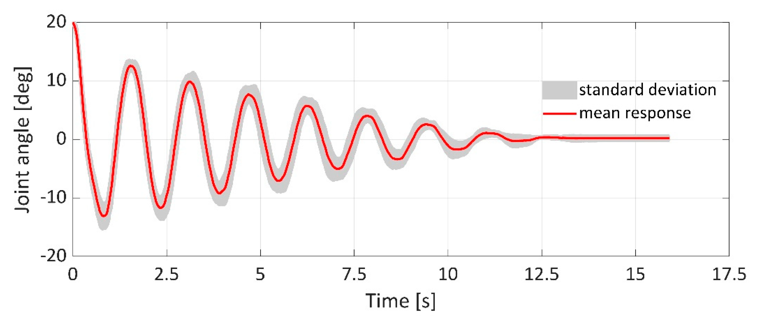
From the 20 measured time courses of the joint angle, where the initial joint angle is 10°, the angles were set for individual measurements in the interval <9.216°; 10.08°>. The maximum value of the interval represents the statistic parameter Mode. Figure 4 represents the mean response (red curve) and standard deviation (the grey area) from measured data.
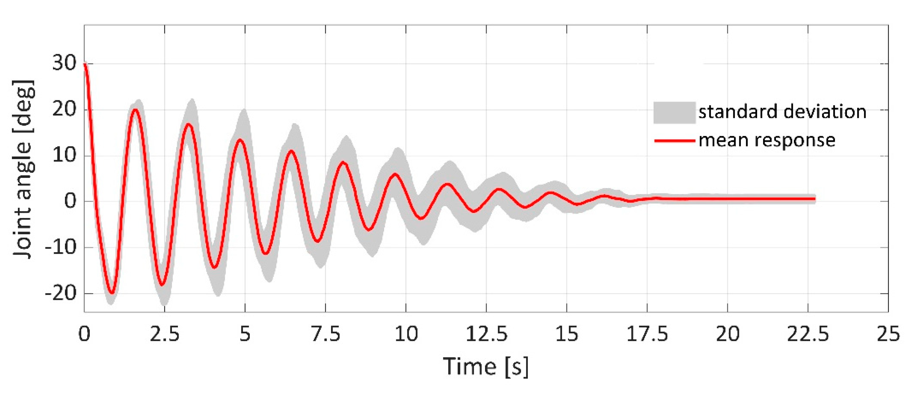
The interval of the initial angles of rotation of the joint with a reference value of 20° was <19.872°; 20.016°>. Such a small range was caused by the fact that out of 20 measurements, the value 20.016° was set 19 times. Waveforms of standard deviation and mean response of data are shown in Figure 5.
Figure 6 shows the waveform of mean response at a joint angle of 30° for link 1, where the initial values of the joint angle were set in the range <29.808°; 30.24°>. More than half of the measurements started from 30.096°. Figure 6 shows a more pronounced standard deviation also (compared to the deviation for angles of 10 ° and 20 °).
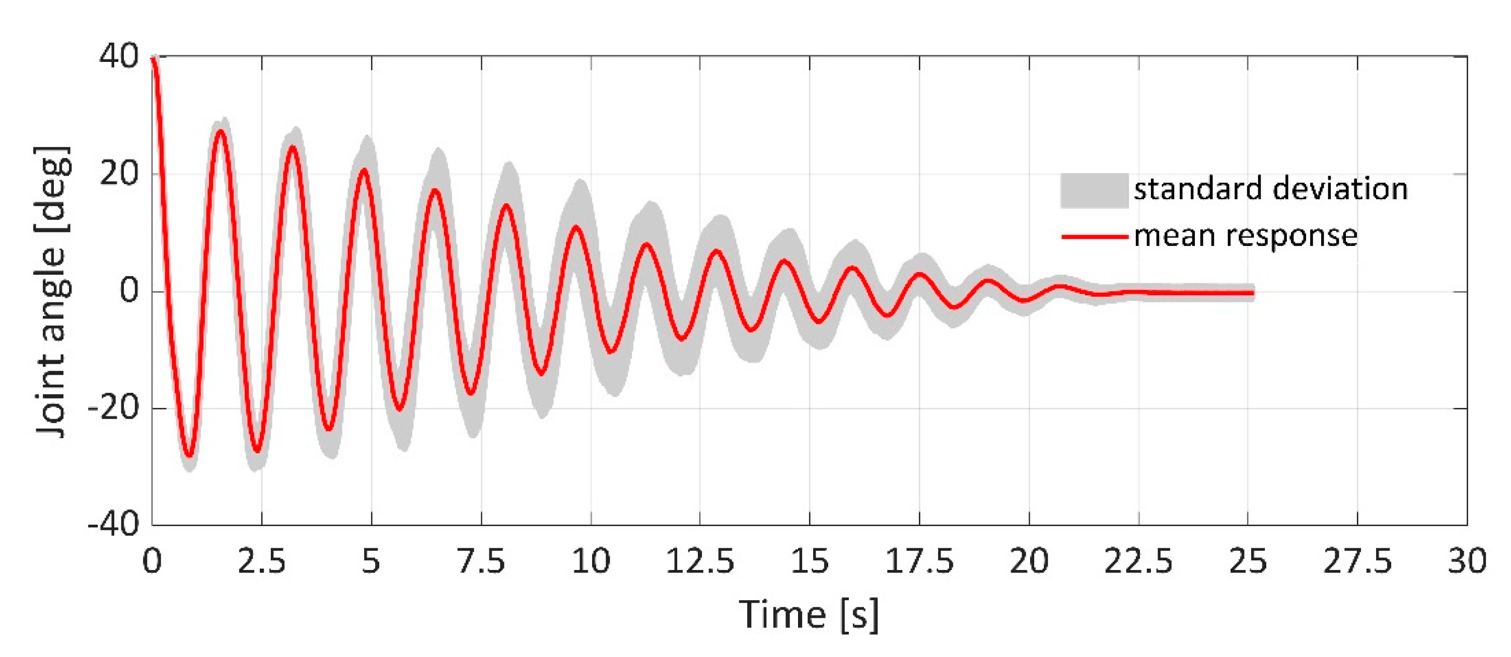
The last group within link 1 is closed by the curve mean response and standard deviation if the initial angle was 40°, as shown in Figure 7 (respectively, in reality, the initial angles were set in the interval <39.888°; 40.464°> during the measurements). Half of the measurements were started at a joint rotation angle of 40.032°.

4.2. Measured Data—Link 2

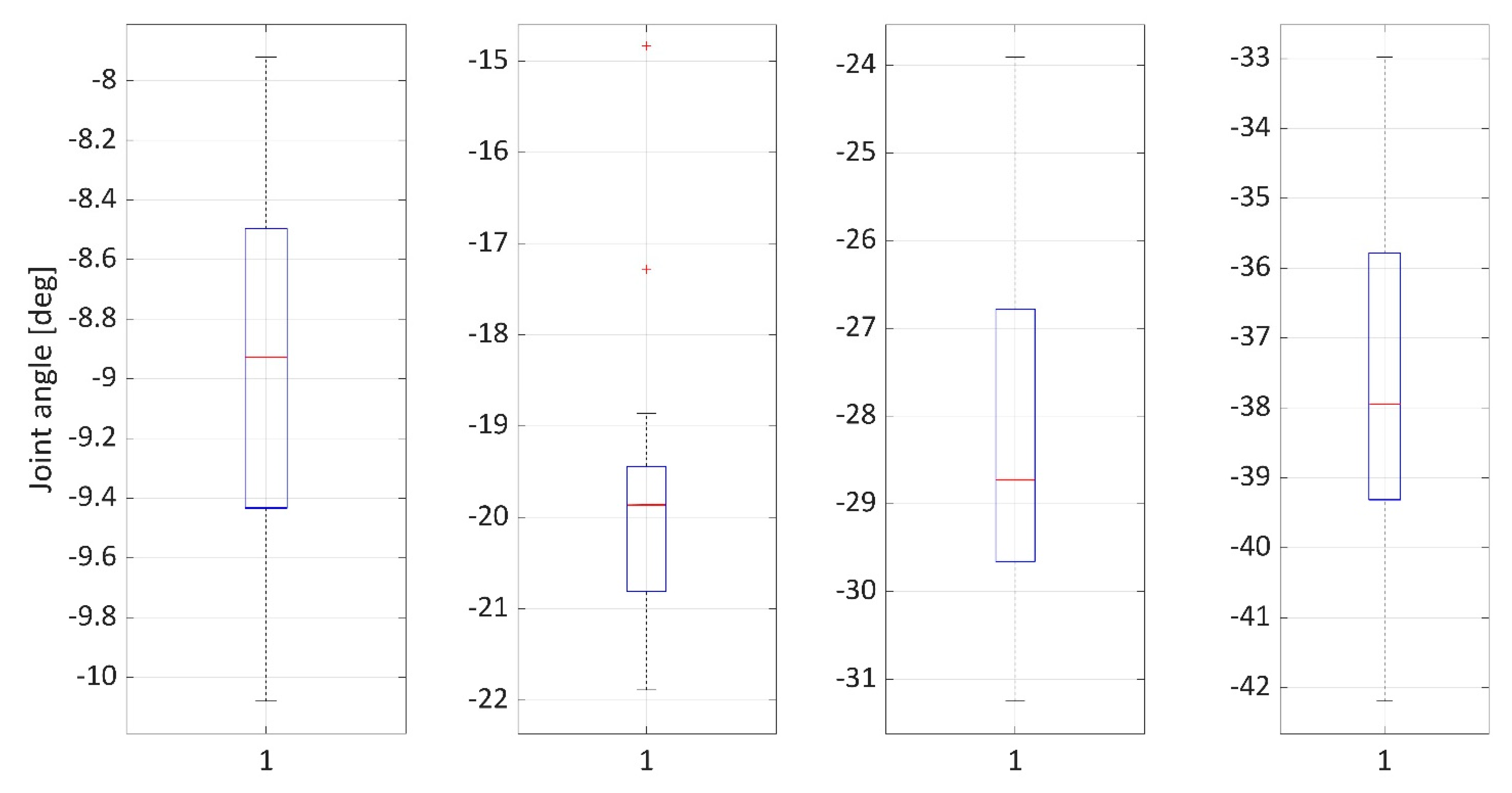
Figure 8 shows four boxplots for link 2 (when viewed from left to right for an initial joint angle of 10° to 40°). In these graphs, in comparison with the graphs for link 1, it can be seen that the minimum and maximum values of the set initial angles are much further apart, which results in a more significant shift of the mean value from the desired initial angle (especially for the angle −40°, fourth graph from the left). The remote value was measured only for an angle of 20° (red crosses, second graph from the left), two times (−17.28° and −14.832°).
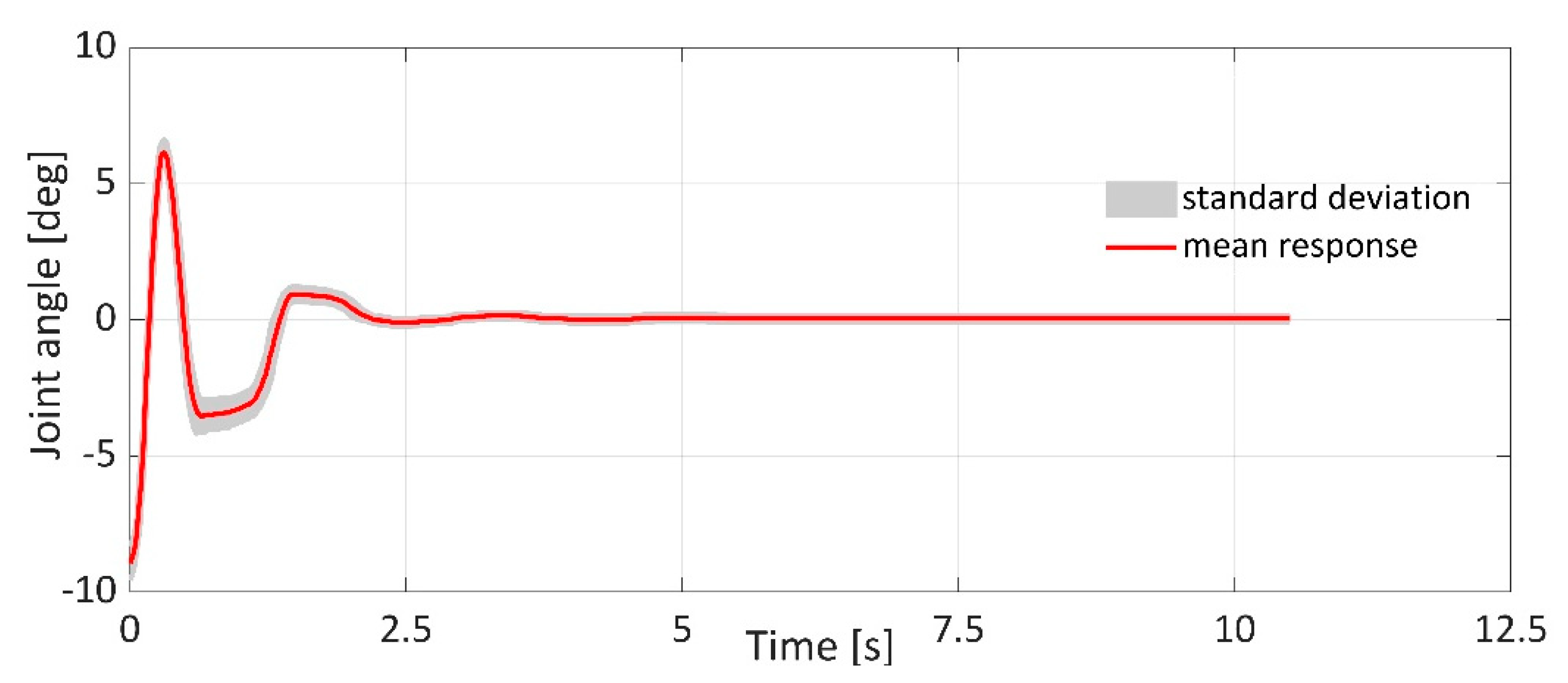
While for link 1, the initial angles were set in the range of up to 1°, the setting of the initial joint angle for the measurements of link 2 was more difficult in terms of constraints in the construction of the system. Figure 9 graphically presents the mean response (red curve) and standard deviation (grey area) when the initial angle was set to −10°. The total interval of the initial values of the angle of rotation was <−7.92°; −10.08°>, the Mode from the twenty initially set angles was −8.928°.
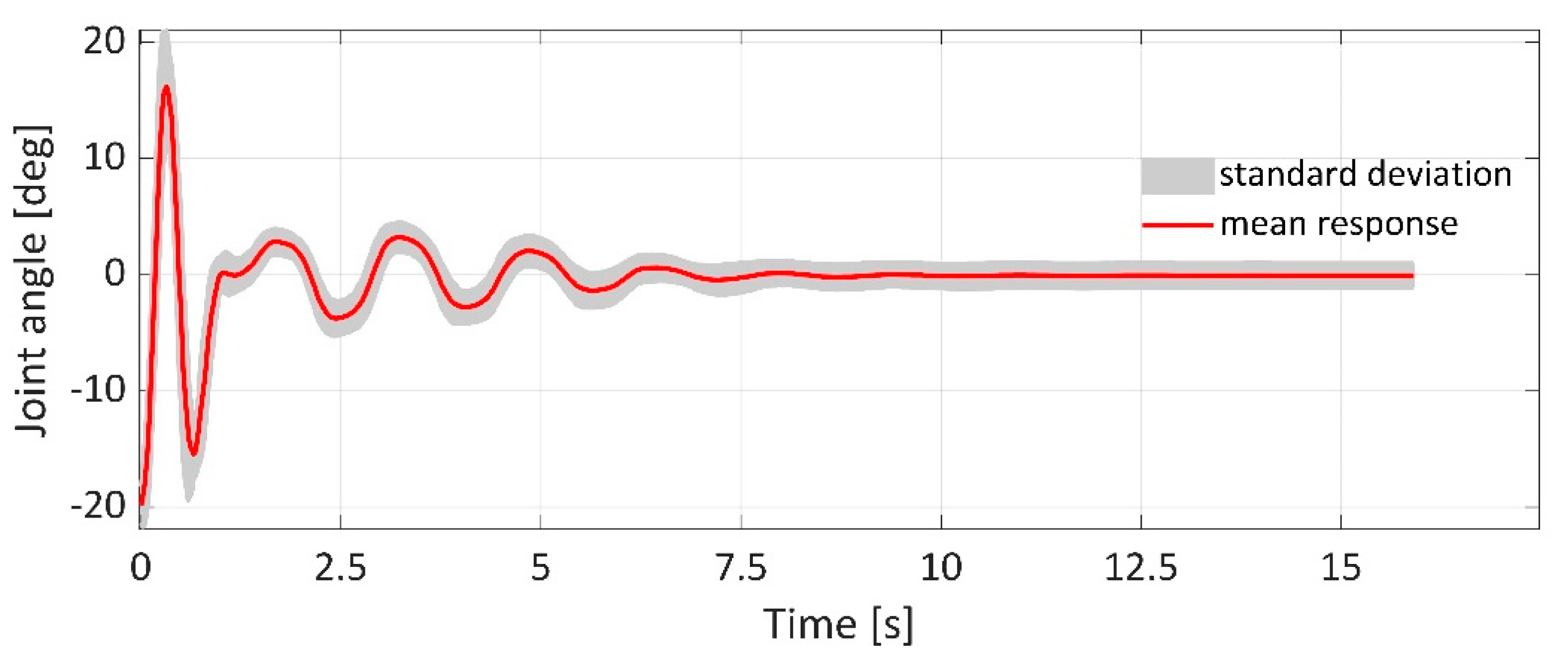
As the joint angle for link 2 increases, the range of the intervals of the initial values of the joint angle also increases (it is also visible in the area of the standard deviation parameter in Figure 10). The interval for the initial value of the joint rotation angle −20° is <−14.832°; −21.888°>, where the difference between the minimum and maximum value of the interval already exceeds 7°. Nevertheless, the value of the Mode parameter (−20.736°) is close to the reference value.
The interval for the reference value −30° for link 2 was <−23.904°; −31.248°>, where from the range of initial values, it is possible to monitor a more significant value of the parameter Mode (−24.048°) in comparison with the reference value. The shift of the beginning of the mean response curve (Figure 11) and the standard deviation area itself is caused by one of the measurements when the initially set value was −23.904 °.
The last measured data was for the initial joint angle was −40°. The total interval of the initial values of the joint angle was <−32.976°; −42.192°>, the Mode of these twenty values was −38.736°. In Figure 12, it is possible to see the fact that the variance in the measurements is the most expressive, which of course, was reflected in the standard deviation.
Gravity tests showed that within link 1, the time course of mean response of the joint angle was more uniform with gradual stabilization to the value of the zero joint angle. For link 2, it is clear from the graphic waveforms that the course is different compared to link 1. A more pronounced stabilization for link 2 for each initial joint angle begins only after a certain amplitude has been exceeded. Additionally, in the case of graphical dependencies, link 2 can see more significant friction, which can affect the validation process. Further, from the sample mean responses and standard deviations for link 1 and link 2, it can be presented that for initial joint angles of 10° and 20°, the standard deviation range is narrower than for 30° and 40° for both axes, which means that at higher initial joint angles, the deviation from the mean response is more pronounced. This could be caused by the stronger manifestation of unmodeled effects, such as additional oscillations of the structure, which was not tightly fastened to the floor (itself slightly uneven). In addition, the larger dispersion of the initial angles had an impact on the wider standard deviation band for link 2 compared to link 1. At the same time, it can be seen from the mean response that the arm stabilization was not completed at 0° in any case due to the effect of friction being more pronounced for this axis. The most visible deviation is for a joint rotation of 20° and 30° for link 1 (Figure 5 and Figure 6). After the phase of implementation of gravity tests and analysis of measured data, the stage of validation in the Matlab and Simulink followed.
In research were used only experiments (not simulation) obtained through gravity tests as a validating agent. However, in the first case, are used parameters values that could be obtained from CAD, and thus could directly be used for simulation without the need for experiments (nevertheless, even in this case, this was validated using the measurements—Chapter 5). In the second case, these parameter values were used as initial values for parameter optimization to obtain an improved model that includes the effects not incorporated in the model with CAD parameters—Chapter 7 (such as fluidic muscles, chains, etc.).

5. Validation

Based on the dynamic model presented in the section Dynamic Model of The System, a simulation scheme in the Simulink was created for the validation process. The basic physical parameters of the system (mass, length, a moment of inertia and distance from the axis of rotation of the joint to the center of gravity for link 1 and link 2) were exported from the CAD software, which was used to make a 3D model of the system. The coefficients viscous friction coefficient and Coulomb friction magnitude were determined experimentally. An overview of these parameters (with parameter designation, value and unit) is summarized in Table 2.
The validation outputs were evaluated based on the MAE (Mean Absolute Error) and NRMSE (Normal Root Mean Square Error) statistical indicators. The indicators are used to compare the output of the model with the outputs of the system. The MAE indicator by a numerical value represents the error that occurred during the validation compared to the measured data. The general mathematical formulation of MAE is given in Equation (7), where yj represents the output of the system on the k-th sample and ӯj represents the output of the model on the k-th sample. The NRMSE, unlike the MAE, compares the degree of agreement of the simulated output with the measured data (Equation (8)). The desired value is for NRMSE = 100% when the model output corresponds 100% to the system output.
M A E = 1 n j = 1 n | y j y ^ j |
F g o f = ( 1 j = 1 n [ y j y ^ j ] 2 j = 1 n [ y j 1 n j = 1 n y j ] 2 ) × 100 %

5.1. Results of Validation—Link 1

The validation results based on the selected MAE and NRMSE criteria for link 1 are summarized in Table 3. The model output for link 1 achieved the best result based on both statistical indicators at an initial joint angle of 10° (MAE = 1.0932 and NRMSE = 35.47%). However, even with the best model, the results represent that the agreement of the model output with the measured data is low and insufficient.
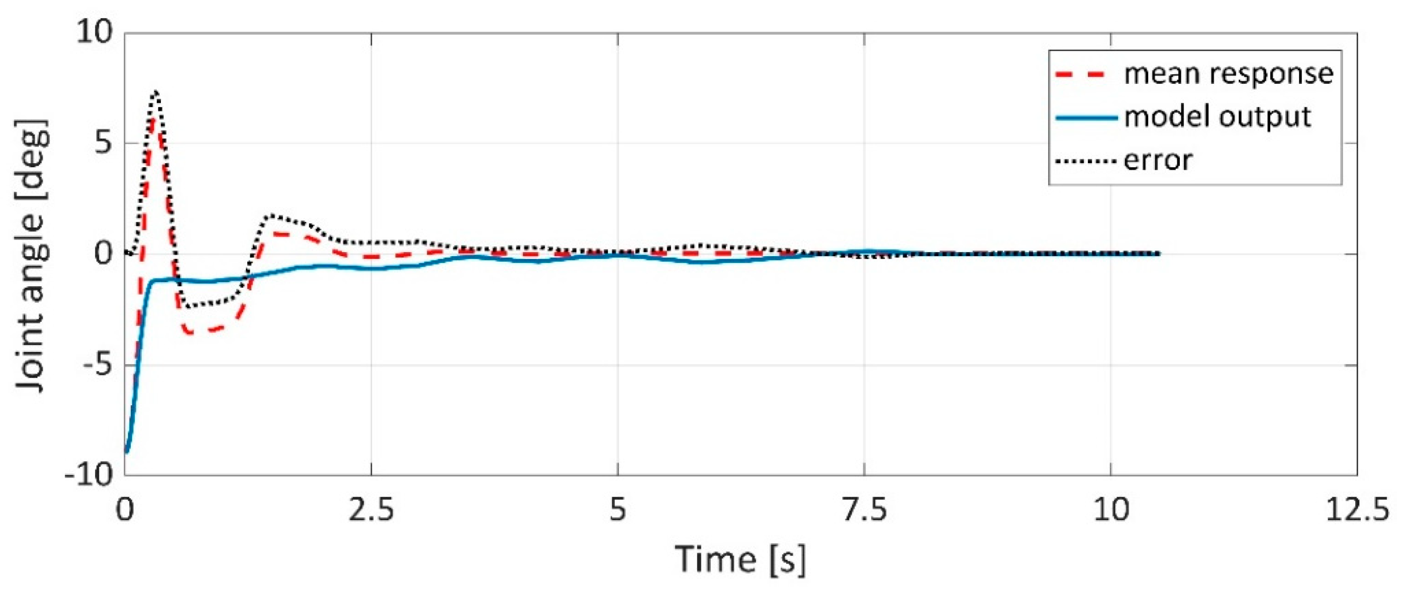
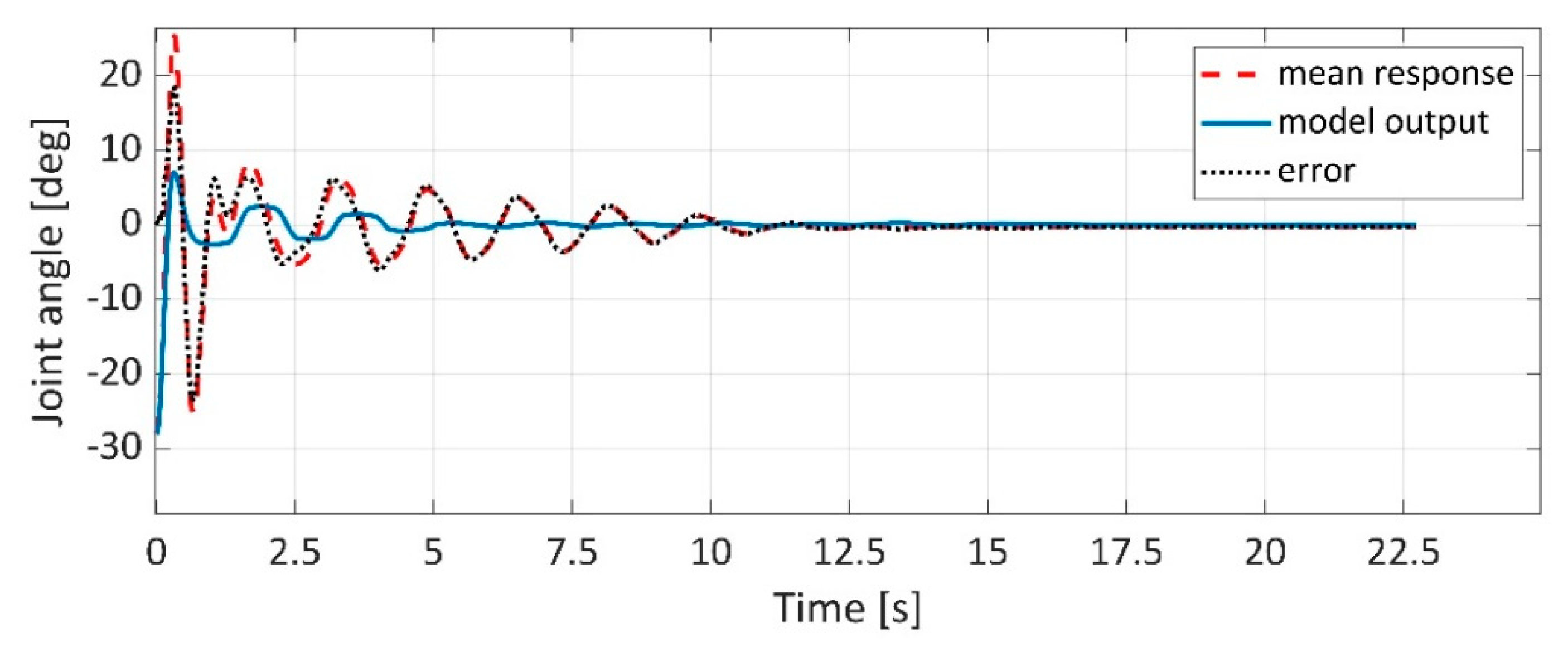
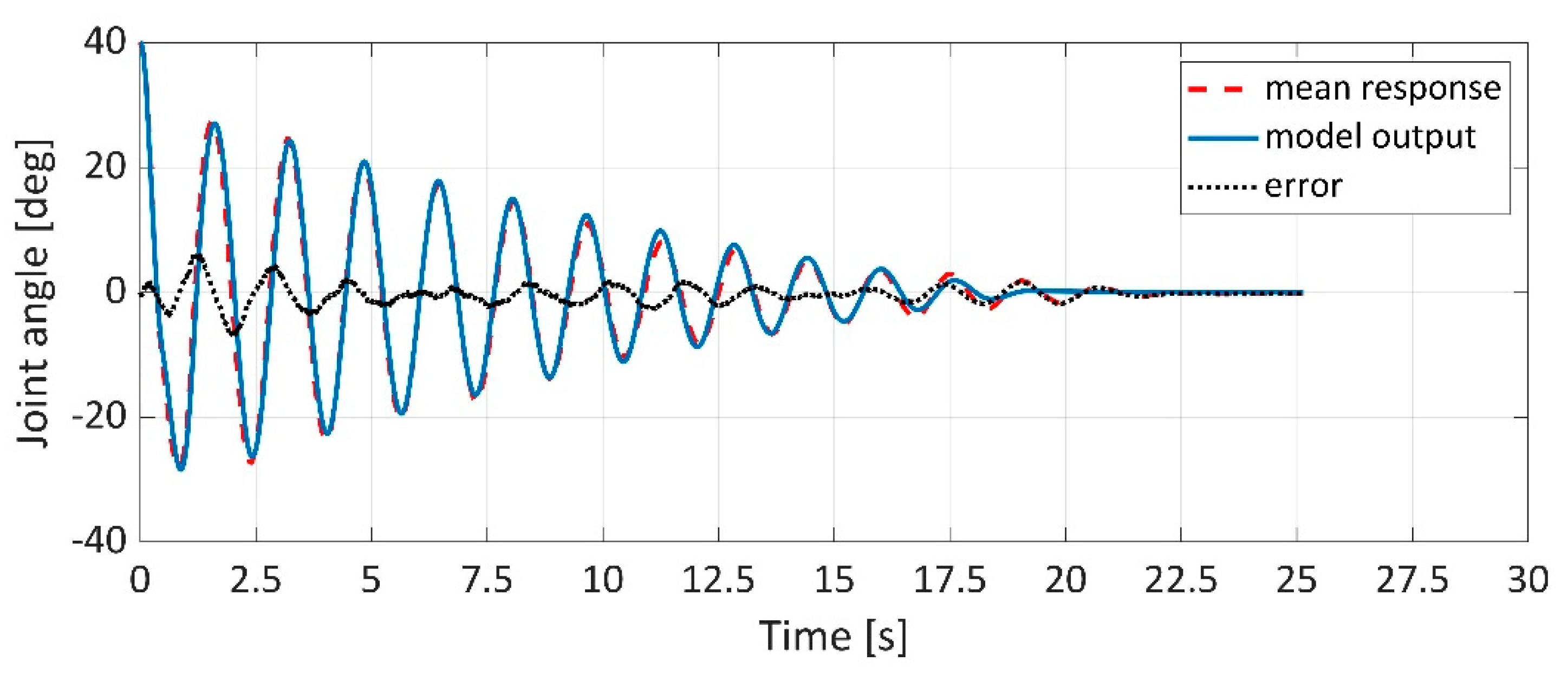
Figure 13, Figure 14, Figure 15 and Figure 16 show the model outputs for the joint 10°–40° for link 1. It can be seen from the waveforms that the model outputs (blue solid line) are largely unable to simulate an expected output represent by mean responses (red dashed line) at the specified input parameters. The error (black dotted line) for a joint angle of 10° has a decreasing tendency with a gradual approach to zero (Figure 13). The error waveforms for the joint angles 20–40° (Figure 14, Figure 15 and Figure 16) are initially smaller but then increase over time, and at the moment when the mean response and thus the output model approaches zero, the value of the error is minimized.

5.2. Results of Validation—Link 2

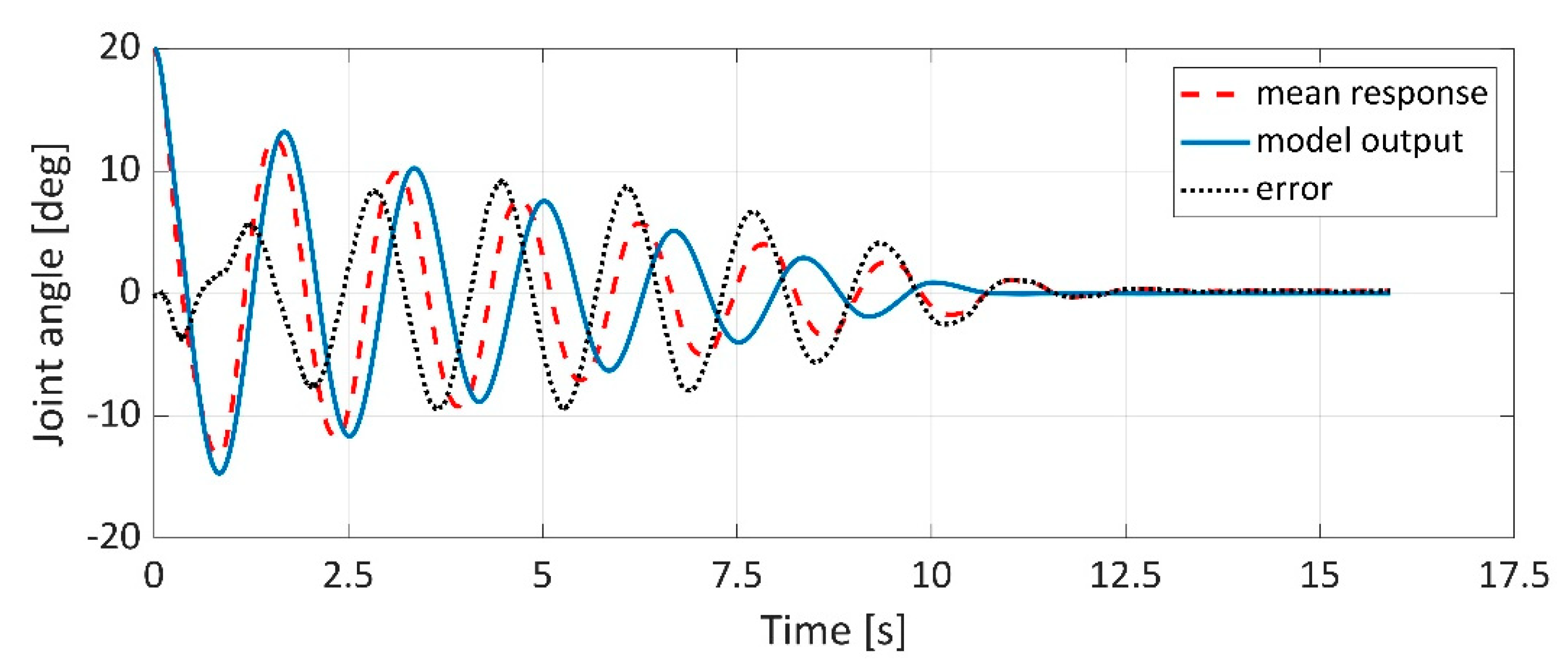
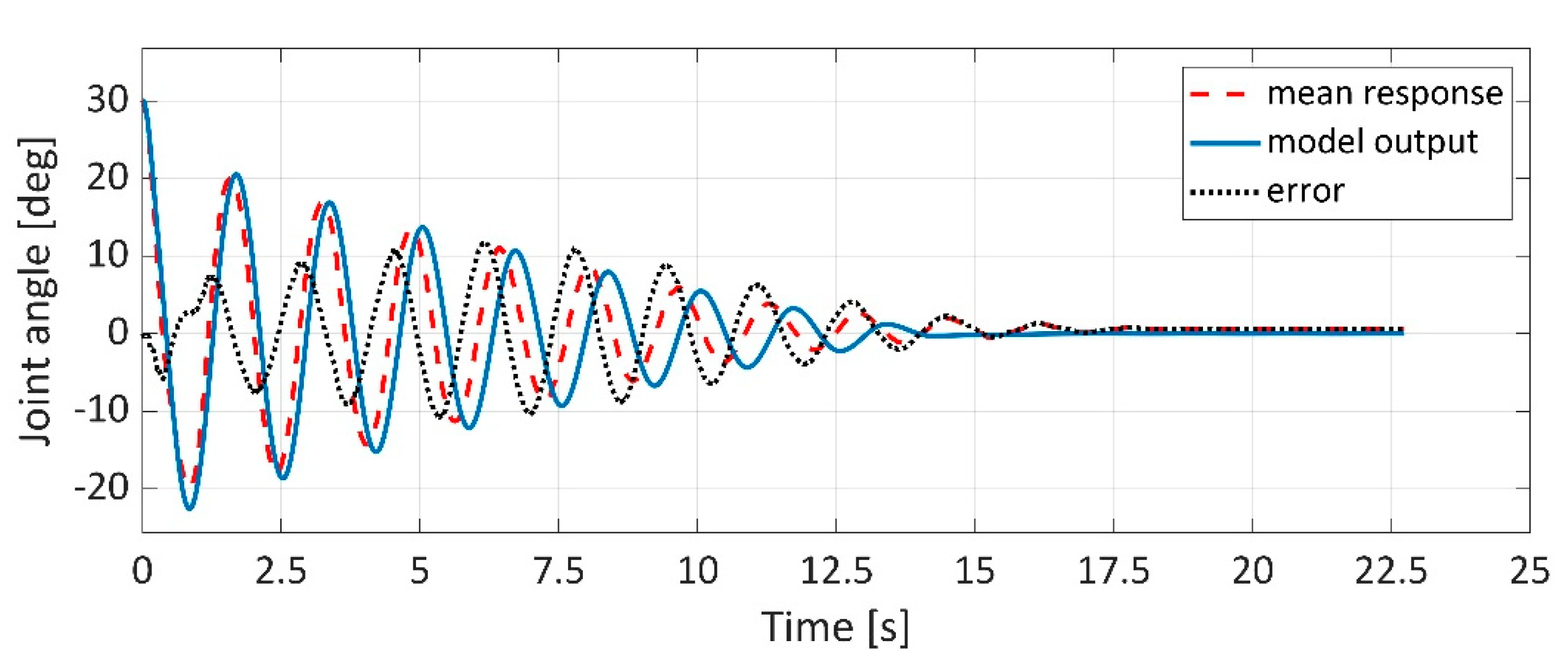
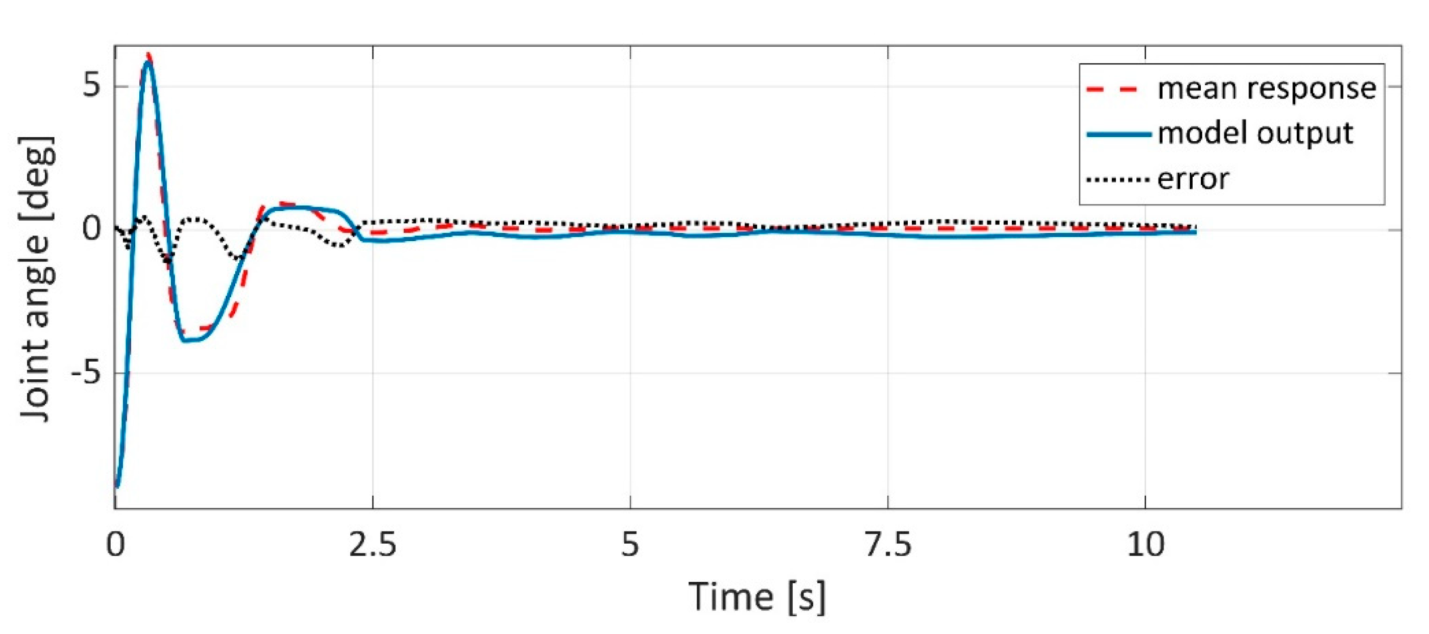
From the analysis of the validation results for link 2 (Table 4) based on the above indicators, it is clear that the values of the indicators achieve even worse results than in the case of link 1 (this may be due to oscillations that originate from the interconnection of individual parts of the system for link 2 as for link 1). The highest value of the indicator NRMSE = 18.14% was achieved for the model when the input joint angle was 30°, but MAE achieved the best result at the initial joint angle of 10° (MAE = 0.5655).
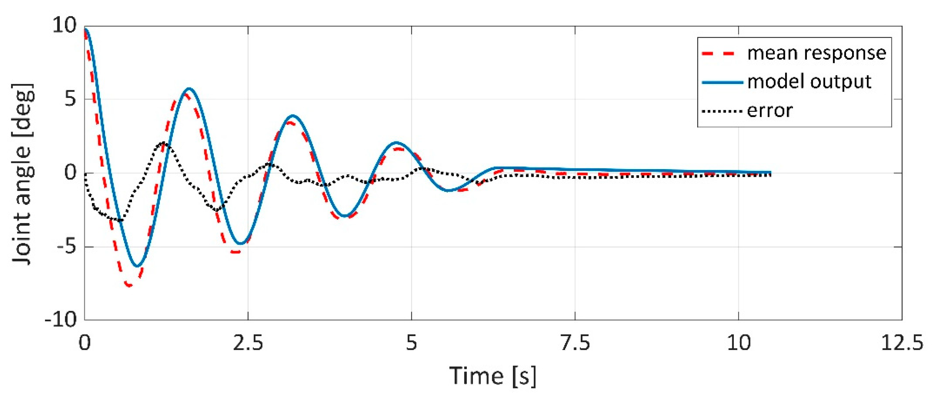
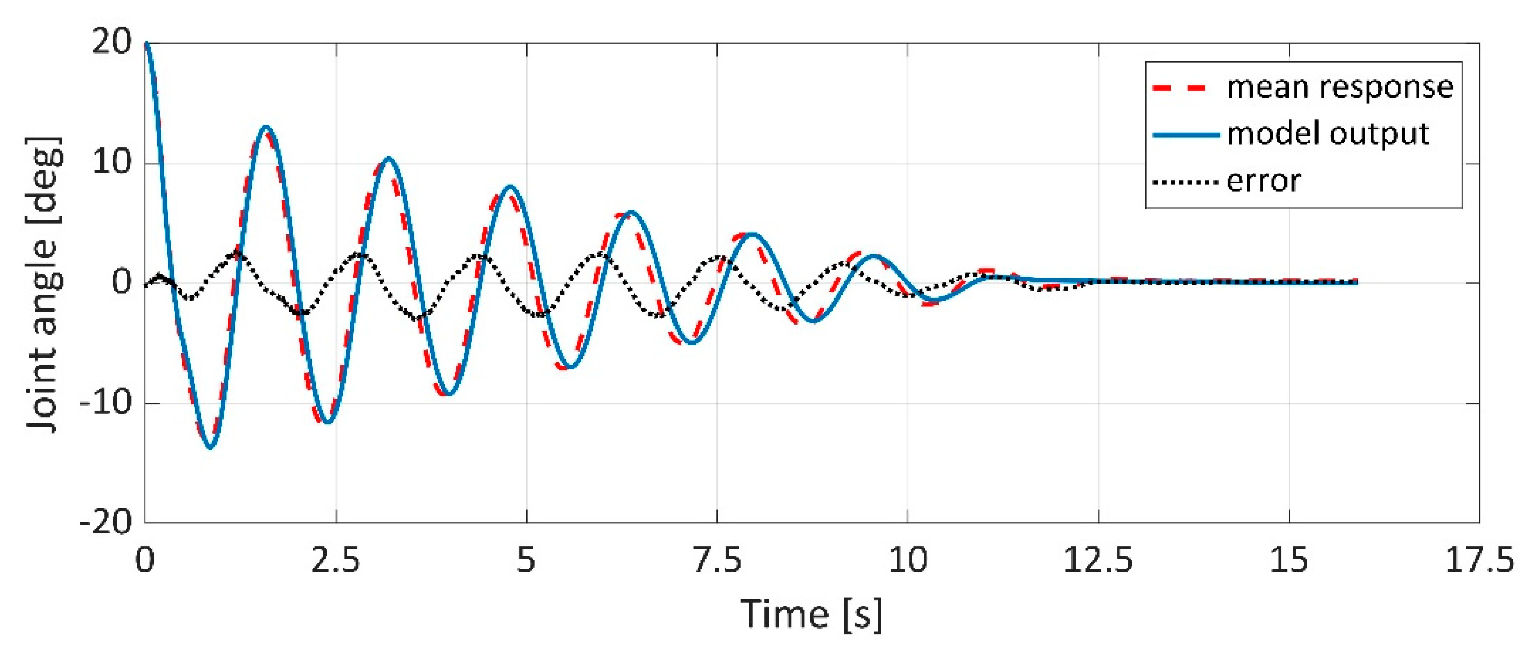
Since the course of the measured data for link 2 has a different character compared to the courses of link 1, and at the same time, a larger oscillation is present, these facts are also reflected in the actual outputs of the model. In Figure 17, Figure 18, Figure 19 and Figure 20, where the model outputs of validation for the joint angle 10–40° for link 2 are presented, it is possible to see to what extent over time the model output (blue solid line) was able to approach an average of the measured values (red dashed line). Since the output of the model moves many times close to the zero value of the joint angle, in all cases, the shape of the error (black dotted line) is similar to the course of the mean response. Similarly, for both link 1 and link 2, at the moment when the mean response and thus also the output model approaches zero, the error value is minimized.
Based on the insufficient results obtained in the validation phase and presented either in the form of MAE and NRMSE criteria parameters or by time dependences of the model outputs alone, compared to the average of measured values and the error between model output and real setpoint, was as next step selected estimation of model parameters. Parameter estimation is an efficient tool that uses mathematical models to accurately describe the behavior of systems. This phase is described in the following two sections.

6. Parameter Estimation of 2-DOF Planar Arm

To estimate the parameters of the model given in Equations (9) and (10), one has to formulate this as an optimization problem. Based on [31], the parameter estimation problem can be formulated as follows: assuming it is a vector of measured values of joint angle λ n λ consisting of K samples, a vector of model parameters θ ¯ n θ has to be found using an optimization algorithm and properly defined objective function. The objective function used in the experiments was a sum-squared type of error function defined as:
(   λ ) = k = 1 K [ θ ¯ ( k ) θ ( k , λ ) ] T [ θ ¯ ( k ) θ ( k , λ ) ]
The purpose of the optimization algorithm is to find the values of parameter vector λ ^ n λ so that
λ ^ a r g   min λ L (   λ )
where L n λ is the parameter space.

Trust Region Algorithm for Nonlinear Least Squares

Nonlinear optimization is the minimization of a function according to the following formulation:
min x R n f ( x )
subject to ci(x) = 0 for i = 1,2,…,me and ci(x) ≥ 0 for i = me + 1,…,m. Functions f(x) and ci(x) hold that they are real, defined in Rn; at least one of them is nonlinear; for the coefficients m and me, it holds that are nonnegative integers, and mme. It holds that, if m = me = 0, the function (Equation (11)) presents an unconstrained optimization problem. If this condition does not apply, then Equation (11) is a constrained optimization problem.
Optimization problems are solved by numerical iteration methods, which means that the approximate solution of the function at the point xk is in the k-th iteration. The new point (approach to the solution) xk+1 is determined computationally based on an algorithm. Such approximation to the solution is applied until the solution is acceptable. An important aspect in the direction of the search, whereby solving subtasks it is verified whether the points are approaching, resp. do not come close to the solution. One of the algorithms that can be applied is the Trust Region Algorithm [32,33,34,35]. The Trust Region Algorithm for Nonlinear Least Squares is similar to the method Levenberg–Marquardt [25,36] used to solve nonlinear functions. Although it is a newer algorithm (compared to Levenberg–Marquardt), it brings advantages such as robustness, reliability and convergence properties. In this algorithm, the model is said to be trusted if the area is close to the solution. Such an area is called a trust region and is modified at each subsequent iteration. This means that if in a certain iteration the approximate model is not good enough (it, therefore, contains a bad point), the area of confidence will not be increased but, on the contrary, will decrease.
After a nonlinear optimization problem was defined using Equation (12), if this problem were unconstrained, the algorithm model could be constructed under the condition that the trial step in the k-th iteration would be determined as [34]:
min d R n g k T d + 1 2 d T b k d = φ k ( d )
Subject   to   d 2 Δ k
where bk is a symmetric matrix of dimension nxn approaching the Hessian of the function f(x); gk represents the gradient at the current iteration xk; ∆k is greater than zero and represents the trust-region radius.
If Equation (13) is subtracted from Equation (12), then the difference is Sk. Subsequently, if the difference φk(0)−φk(Sk) is determined, the result is Pk, which represents the predicted reduction. For Pk, holds it is positive if xk is a stationary point and bk is a positive semi-definite. Actual reduction Ak (reduction in objective function) can be determined as Algorithm 1 [34]:
A k = f ( x k ) f ( x k + S k )
If the ratio is the actual reduction Ak and the predicted reduction Pk, it is obtained an important ratio rk, which firstly expresses whether the test step is acceptable and secondly determines the adaptation of the new trust-region radius.
Algorithm 1 [34]
  •  Step:     Given:   x 1 R n ,   Δ 1 > 0 ,   ϵ 0 ,   b 1 R n x n ;

                0 < τ 3 < τ 4 < 1 < τ 1 ,   0 τ 0 τ 2 1 ,   τ 2 0 ,   k 1
2.
 Step:     If      g k 2 ϵ then stop;

                   Solve is Sk
3.
 Step:     Calculated r k = A k / P k

                x k + 1 = { x k          i f   r k τ 0 x k + S k        o t h e r w i s e
Choose   Δk+1 that satisfies
                Δ k + 1 { [ τ 3 g k 2 , τ 4 Δ k ]      i f   r k < τ 2 Δ k ,   τ 1 Δ k       o t h e r w i s e
4.
 Step:     Update

               bk+1; k: = k+1;   go to 2. Step.
τi is chosen by the user (usually τ0 = 0, τ1 = 2, τ2 = τ3 = 0.25, τ4 = 0.5). Normally, τ0 is chosen to be zero, but if τ0 >0, count of lim k i n f   g k 2 = 0 will be stronger. As a satisfactory optimal criterion for terminating the algorithm at point xk is g k 2 ϵ .

7. Parameter Estimation of Simulink Model

Within the estimation of model parameters, attention, in this case, was focused on the parameter estimation of the Simulink model, where the task is to process the input/output data used for the testing phase. In the validation phase, tests were performed separately for link 1 and link 2 and at the same time for each axis at four different initial joint angles. However, when estimating the model parameters, the estimation takes place simultaneously for link 1 and link 2 for the specified joint angle. To create the experiment, it was necessary to select the measured outputs—the matrix of the required measured outputs depending on time. Specifically, in this case, it was the time dependence of the mean response obtained from the measured data. Another important step in configuring the experiment was to choose which parameters to estimate. In the performed experiment, all physical parameters of the system were selected for estimation, which are listed in Table 5. At the same time, it was necessary to determine the limits of the set parameter. The limits were set to ±30% of the original parameter values obtained from the CAD software (excluding friction). The basis of parameter estimation is an optimization method and algorithm that determine the sequence of steps in which the estimation takes place and what criteria for parameter estimation are chosen. Based on what was mentioned in Section 4, the Trust Region Algorithm for Nonlinear Least Squares was chosen.
The result of parameter estimation is new estimated values of selected model parameters, which were reused for validation to obtain better model results. An overview of these parameters is summarized in the list of model parameters after parameter estimation in Table 6. The simulation scheme in Simulink was modified with new detected parameters, and the process of output validation based on measured data was performed as in section Validation. The results of the validation after estimating the parameters are divided into two parts—for link 1 and link 2.

7.1. Results of Validation after Parameter Estimation—Link 1

The results of validation after the estimation of parameters were assessed based on the same statistical criteria as in the validation before estimation. Table 7 provides an overview of the MAE and NRMSE indicators for link 1. From the results, it can be seen that based on the MAE indicator, the model at the initial joint angle of 10° (MAE = 0.6076) is the best, while based on the NRMSE indicator, it is the model at an initial joint angle of 40°, with NRMSE = 84.62%.
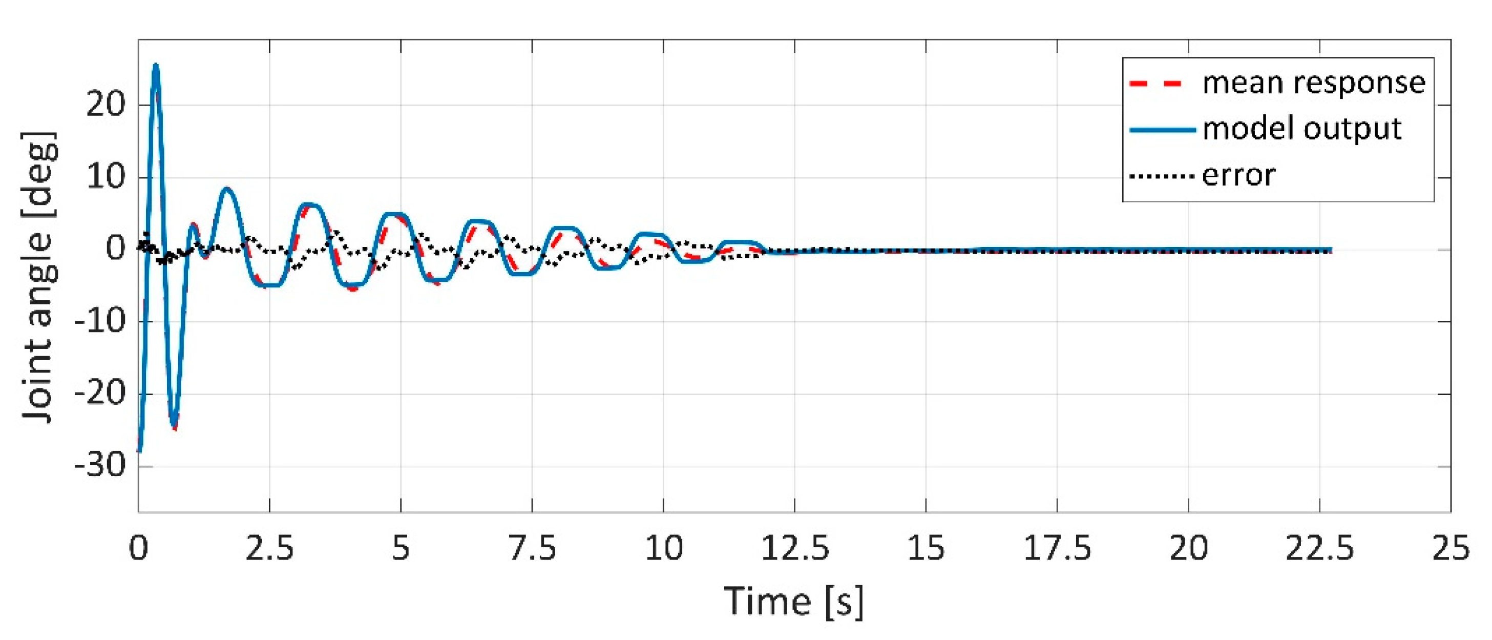
The improvement of the model results is obvious also from the graphic curves. Figure 21, Figure 22, Figure 23 and Figure 24 show the model outputs after parameter estimation for the joint 10°–40° for link 1. The model output (blue solid line) approaches the required mean response (red dashed line) with increasing initial joint angle, which also indicates an increase in the value of the NRMSE indicator in Table 7. Before estimating the parameters, the model output had the problem of achieving mean response amplitudes and also the peaks of the model output amplitudes that were shifted for the time axis.

7.2. Results of Validation after Parameter Estimation—Link 2

The results of the validation before estimating the parameters were significantly worse for link 2 compared to the results for link 1. However, after estimating the parameters and performing the validation again, the models were able to produce much better model outputs, as evidenced by the MAE and NRMSE values in Table 8. The MAE indicator had a value of less than one for each initial joint angle, with the best output of the model obtained at an initial joint angle of 10° (MAE = 0.2407). The value of the NRMSE indicator was around 80% at all initial joint angles examined, with the model achieving the best result at an angle of 20° (NRMSE = 82.82%).
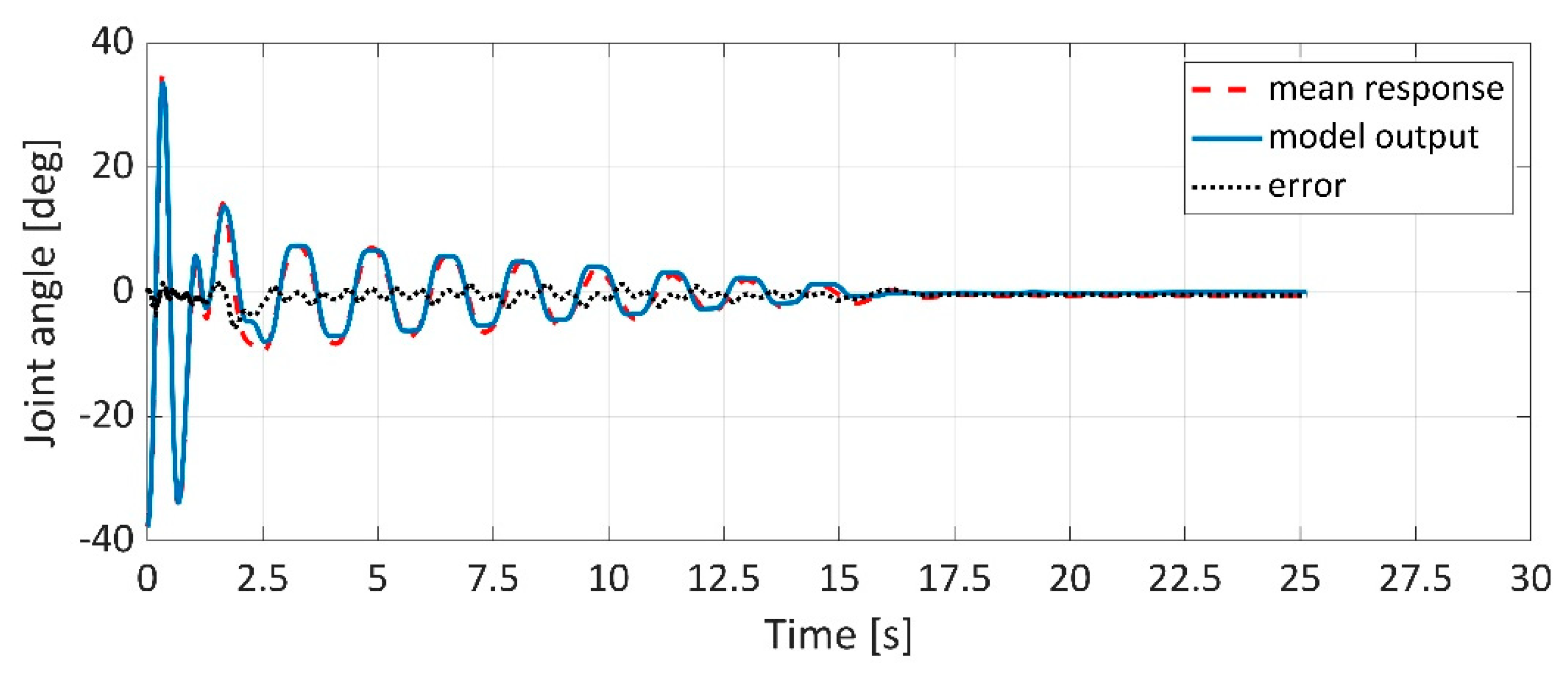
This significant difference in the improvement of the model results after parameter estimation is especially visible in Figure 25, Figure 26, Figure 27 and Figure 28. The model before parameter estimation had the biggest problem for link 2 with data in the time zone 0 to 2.5 s when there are significant fluctuations of the manipulator’s arm. However, these jumps are followed by more pronounced damping. However, the model after estimation can simulate the output (blue solid line) at this time with high accuracy to the mean response (red dashed line) for each initial joint angle, which is of course also reflected by the change in the curve error (black dotted line).

8. Discussion

The estimation of model parameters using the Trust Region Algorithm for Nonlinear Least Squares optimization method for the known structure of the planar kinematic system model derived based on Lagrange formalism was intended to improve the validation results. As mentioned above, the limits of the estimated parameters were set to ±30% of the original value of each parameter (excluding friction). This value was set because deviations could occur within the parameters specified by the CAD software, e.g., the resulting weights can be skewed, as an element, such as a chain or muscles, is not included in the CAD. CAD, therefore, determined the parameters only based on the modeled construction. A summary and comparison of validation results before and after parameter estimation is given in Table 9 for link 1 and in Table 10 for link 2. It is clear from the indicators that the estimation of parameters significantly helped to achieve better model outputs in the process validation. If the indicators for link 1 are compared, the most significant improvement occurred at the initial joint angle 40°, when the original output of the model reached MAE = 6.1717 and NRMSE = 16.69%, while after estimation, the output of the model was obtained at MAE = 1.1045 and NRMSE = 84.62%. For link 2, the results in the initial validation were even worse than for link 1. As mentioned above, the cause could be a more pronounced oscillation in this axis. Therefore, this fact was expected to play a role in the results even after optimization. However, it is clear from the results that the optimization within the parameter estimation helped the model so much that the outputs not only achieved much better results than before the estimation, but within the NRMSE indicator, they were also similar in value (stable) at different initial rotation angles. However, the most significant change after the determination occurred at an initial angle of 40° (taking into account the values of both indicators).
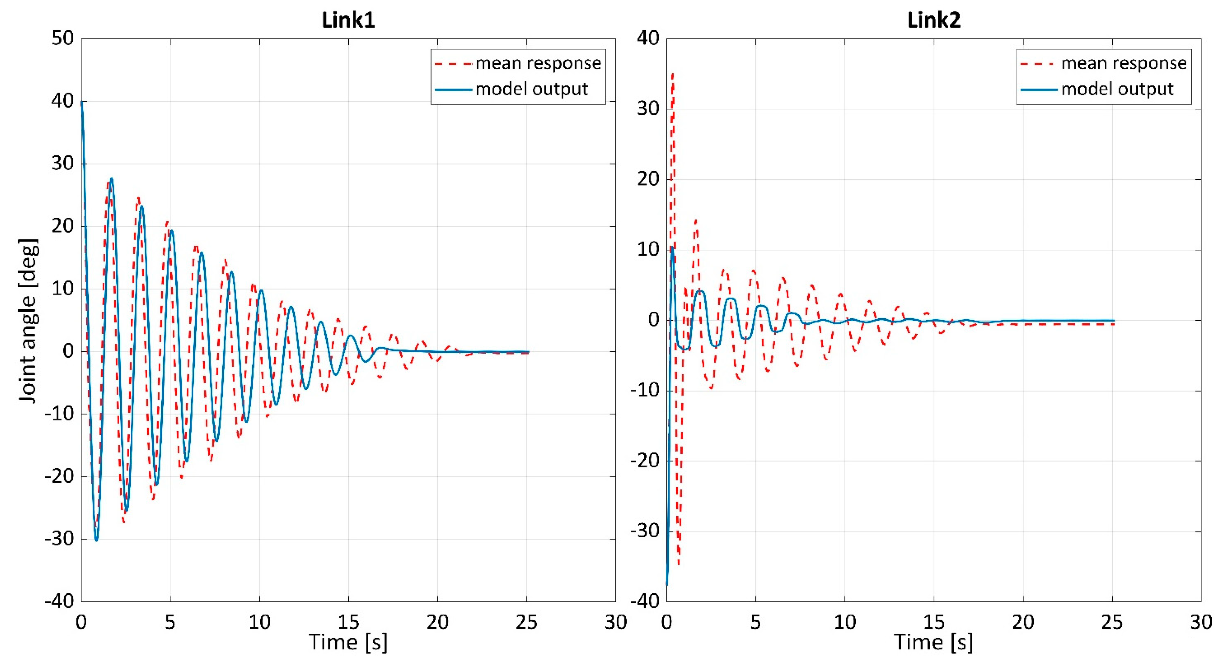
Since the process of estimating the parameters took place simultaneously for both axis 1 and axis 2, from the results of the estimation, it was necessary to select the model that achieved the best results as a whole (not separately for axis 1 and axis 2). As already mentioned at the beginning of this chapter, the most significant progress in the results occurred at the initial angle of rotation of the joint of 40°, so this model was chosen as the best. Figure 29 shows the time courses of the joint angle for both axes at the initial joint angle of 40° before the model optimization process. For both axes, you can see that the output model (blue solid curve) is different compared to the required mean response (red dashed curve). After optimizing the model, however, significant differences (improvements) for both axes can be seen in the model outputs in Figure 30. The output of the model no outrun the required output (this phenomenon was visible especially for axis 1 before estimation). The model also achieves the amplitude of the measured values much better (especially with axis 2 before estimation, this problem is visible).
Since the essence of the optimization of the model was the estimation of the model parameters using the chosen algorithm, it is important to analyze the estimated parameters themselves, which ensured the improvement of the results. These were the parameters of the manipulator together with the coefficients found in the friction components. In connection with this, it should be noted that since the goal was set in the validations—the best possible model outputs and results within the indicators. Therefore the arm parameters, such as length, weight, etc., were also included in the estimation. Table 11 shows a comparison of the values of these parameters before estimation and after estimation.
The weights of the arm parts m1 and m2 were changed by the estimation—the weight of the upper part of the arm was estimated to 0.9 kg extra, while the weight of the lower part of the arm was estimated to be 0.076 kg less. The parameter, Distance to the center of mass, for both links were increased by a value of 0.053 m for c1 and a value of 0.022 m for c2. The length of the arm on axis 1 is less by 0.063 m. Due to these changes, of course, the values of the moments of inertia I1 and I2 have also changed. The Viscous friction coefficient and Coulomb friction magnitude were set experimentally before the validations. However, after optimization, the values of the Viscous friction coefficient and Coulomb friction magnitude are smaller than the initial value of 0.35 (especially the value of fd2).
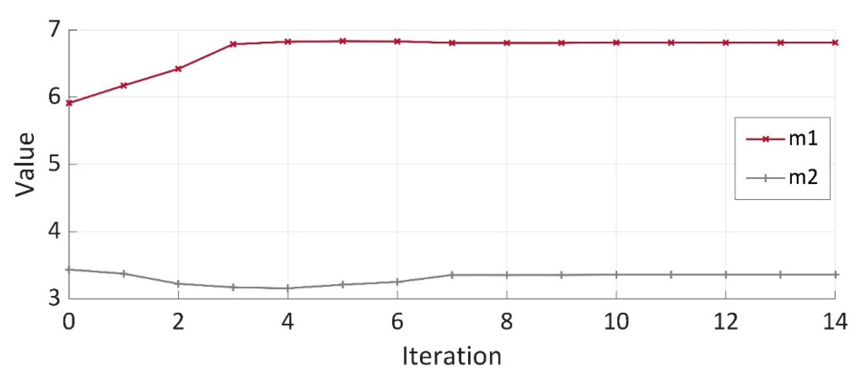
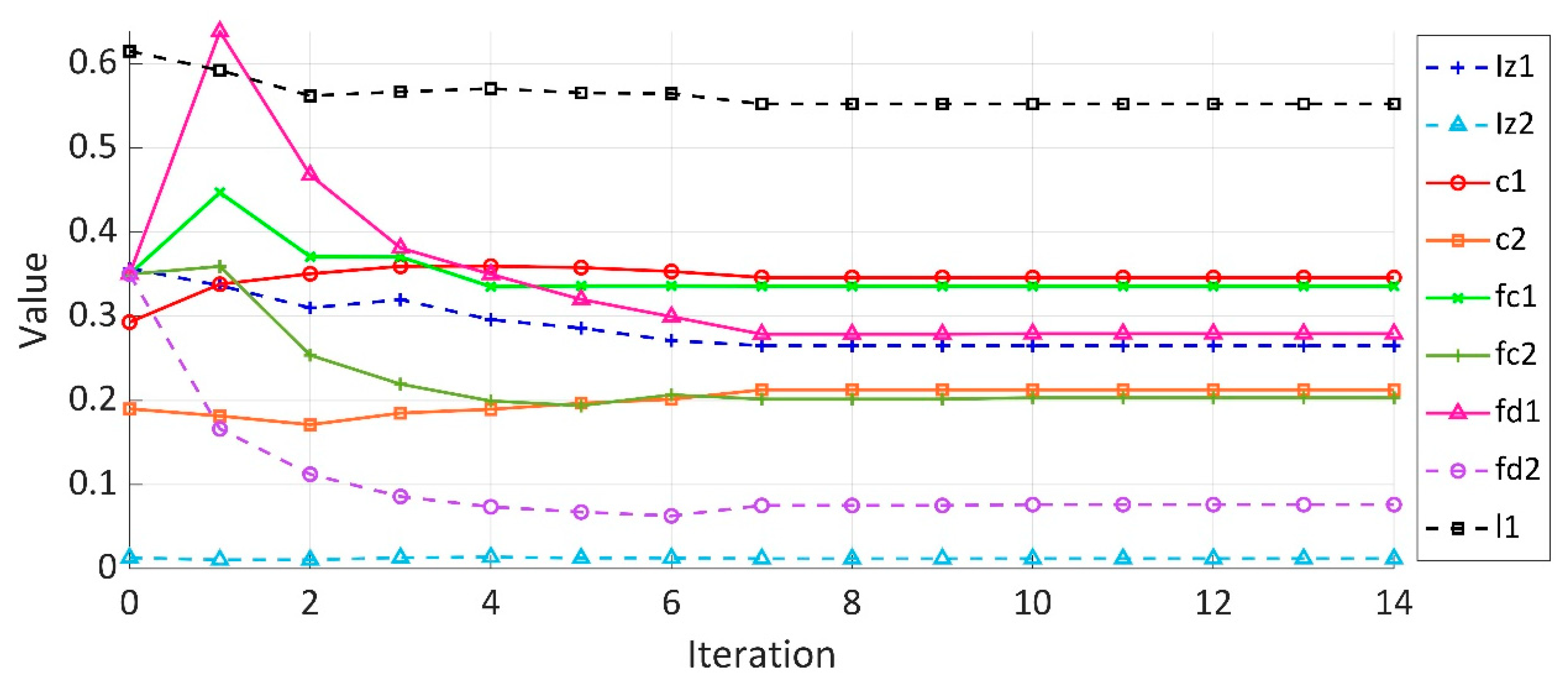
The parameters that were the subject of estimation and used for the subsequent optimization of the model were estimated in the Parameter Estimator. During the estimation process, this tool (among other things) offers the possibility to monitor how the values of the parameters are estimated (changed) depending on the iterations until all the values of the estimated parameters are stabilized. The result of this phase from the given toolbox can be seen in Figure 31 and Figure 32. During the estimation, only one graph could be viewed, where the waveforms of all 11 estimated parameters were. However, since the masses m1 and m2 are represented by much higher values than the remaining parameters, the mass curves were exported to the second graph for better clarity. Based on the waveforms of Figure 32, it can be seen that the smallest changes in the parameter estimation occurred in the parameters c2 (Distance to the center of mass for link 2) and Iz2 (Moment of inertia for link 2). On the contrary, significant changes took place in the values of Coulomb friction magnitude fd1, fd2. In Figure 31, it is possible to observe how the weight estimate has changed. From the course of estimating the mass m2, it can be seen how the weight changed in the first iterations, but the result of the estimation in the last iteration was, in the end, very similar to the original value.
Significant estimates and changes in some parameters can be evaluated based on the following hypotheses:
  • The weights m1 and m2 that were exported from the CAD software did not take into account the total weight of the arms even with connected muscles, chain, etc. Based on which the resulting weight could increase by estimation (this phenomenon is visible especially for axis 1—weight m1).
  • Given the first hypothesis, it is possible to follow up. By changing the weight and shape of the arm, its length, the estimation of the parameter Distance to the center of mass for link 1 and 2—c1 and c2 (a visible increase of these parameters during estimation) is influenced.
  • Changes in the estimation of the moment of inertia parameters Iz1 and Iz2 may also be closely related to the change in mass and the shift of the center of gravity.
  • In terms of the use of a chain and a sprocket, it was assumed that the friction would be more pronounced (than if another gear had been used), so the value of the coefficients was set to 0.35. However, it is clear from the estimation that the experimentally determined initial values of the friction coefficients were oversized, as evidenced by the courses of the estimated parameters fc1, fc2 and fd1, fd2.

9. Conclusions

The research described in this article aimed to compare the model with the parameters that come from CAD and its improvement by estimating the parameters based on gravitational measurements. An improvements model could be subsequently applied to the control phase.
The study described in this article can be summarized in four stages:
  • Obtain a representative set of joint angle data by performing gravity tests.
  • Creation of a simulation model in the Matlab and Simulink, which presented the dynamics of a real system—a planar robotic arm with two degrees of freedom (taking into account the friction component).
  • The validation of a dynamic model built based on Lagrange formalism. However, at this stage, the expected results based on the MAE and NRMSE indicators were not achieved.
  • The estimation of parameters—as the initial results of validation were insufficient, the research was extended to the estimation of model parameters using the Trust Region Algorithm, which helped to significantly improve the values of MAE and NRSME.
Based on the results of parameter validation and estimation, it can be stated that the values of system parameters, which serve as input data for the model, significantly affect the validation results, which was demonstrated after estimating these parameters significantly affected the results. Within the course of the estimated parameters, a certain connection between the parameters was seen, which gives rise to the assumption that the values of the parameters not only influence the results of the validation but also interact with each other. The more accurate the system parameters are obtained in the step, the more accurate the validation results will be. By reducing the oscillations (especially for link 2 and at higher initial rotation angles) which occur in the system due to the individual structural bonds, it would be possible to achieve a more accurate stabilization of the arm movement to zero, and thus to improve the validation results.
In further research, the authors would like to extend this research to the following parts:
  • Accurate identification of system parameter values, including drive parameters.
  • The inclusion of drive dynamics, which would create a more complex dynamic system model.
  • The addition of a part of the drives to the simulation scheme in Simulink, the use of other tools, such as SimMechanics.

Author Contributions

Conceptualization, A.H. and M.T.; methodology, A.H.; model design, M.T. and T.Č.; measuring data, A.H. and T.K.; validation in Matlab, T.Č.; estimation in Matlab, T.Č.; formal analysis, M.T.; investigation, M.T.; writing—original draft preparation, M.T.; writing—review and editing, M.T., A.H., T.K. and T.Č.; visualization, M.T. and T.Č.; project administration, T.K.; funding acquisition, A.H. All authors have read and agreed to the published version of the manuscript.

Funding

The project was supported by the Project VEGA no. 1/0393/18—Research of Methods for Modeling and Compensation of Hysteresis in Pneumatic Artificial Muscles and PAM-actuated Mechanisms to Improve the Control Performance Using Computational Intelligence and by the Project of the Structural Funds of the EU, ITMS code: 26220220103.

Conflicts of Interest

The authors declare no conflict of interest.

References

  1. Liu, C.; Tang, T.; Lin, H.-C.; Tomizuka, M. Designing Robot Behavior in Human-Robot Interactions, 1st ed.; CRC Press: Boca Raton, FL, USA, 2019; ISBN 978-0-367-17969-4. [Google Scholar]
  2. Gasparetto, A.; Ceccarelli, M. Mechanisms and Machine Science. In Mechanism Design for Robotics: Proceedings of the 4th IFToMM Symposium on Mechanism Design for Robotics; Springer: Cham, Switzerland, 2019; ISBN 978-3-030-00364-7. [Google Scholar]
  3. Kroff, J. Modern Robotics: Designs, Systems and Control; Willford Press: Forest Hills, NY, USA, 2019; ISBN 978-1-68285-676-5. [Google Scholar]
  4. Yang, C.; Ma, H.; Fu, M. Advanced Technologies in Modern Robotic Applications; Springer: Singapore, 2016; ISBN 978-981-10-0829-0. [Google Scholar]
  5. Miller, R.; Miller, M. Robots and Robotics: Principles, Systems, and Industrial Applications, 1st ed.; McGraw-Hill Education: New York, NY, USA, 2017; ISBN 978-1-259-85978-6. [Google Scholar]
  6. Ross, L.T.; Fardo, S.W.; Walach, M.F. Industrial Robotics Fundamentals: Theory and Applications, 3rd ed.; Goodheart-Willcox Publ: Tinley Park, IL, USA, 2017; ISBN 978-1-63126-941-7. [Google Scholar]
  7. Colombo, R.; Sanguineti, V. Rehabilitation Robotics. Elsevier Science Publishing Co., Inc.: Amsterdam, The Netherlands, 2018; ISBN 978-0-12-811995-2. [Google Scholar]
  8. Barrett, L. Recent Advances in Robotics; NY Research Press: Forest Hills, NY, USA, 2020; ISBN 978-1-63238-723-3. [Google Scholar]
  9. Kurfess, T.R. Robotics and Automation Handbook; CRC Press: Boca Raton, FL, USA, 2018; ISBN 978-1-4200-3973-3. [Google Scholar]
  10. Siciliano, B.; Khatib, O. Springer Handbook of Robotics; Springer: Heidelberg, Berlin, 2016; ISBN 978-3-319-32552-1. [Google Scholar]
  11. Barrett, L. Handbook of Robotics; Willford Press: Forest Hills, NY, USA, 2020; ISBN 978-1-68285-776-2. [Google Scholar]
  12. Hurmuzlu, Y.; Nwokah, O.D.I. The Mechanical Systems Design Handbook: Modeling, Measurement, and Control; CRC Press: Boca Raton, FL, USA, 2017; ISBN 978-1-4200-3674-9. [Google Scholar]
  13. Nezhad, M.N.; Korayem, A.H. Dynamic Modeling of Industrial Manipulator Hyundai HS165 in Order to Determine the Dynamic Load-Carrying Capacity for a Specified Trajectory. In Proceedings of the 7th International Conference on Robotics and Mechatronics (ICRoM), Teheran, Iran, 20–21 November 2019; pp. 538–543. [Google Scholar]
  14. Varela-Aldás, J.; Andaluz, V.H.; Chicaiza, F.A. Modelling and Control of a Mobile Manipulator for Trajectory Tracking. In Proceedings of the International Conference on Information Systems and Computer Science (INCISCOS), Quito, Ecuador, 13–15 November 2018; pp. 69–74. [Google Scholar]
  15. Leborne, F.; Creuze, V.; Chemori, A.; Brignone, L. Dynamic Modeling and Identification of an Heterogeneously Actuated Underwater Manipulator Arm. In Proceedings of the IEEE International Conference on Robotics and Automation (ICRA), Brisbane, Australia, 21–25 May 2018. [Google Scholar]
  16. Hošovský, A.; Piteľ, J.; Židek, K.; Tóthová, M.; Sárosi, J.; Cveticanin, L. Dynamic Characterization and Simulation of Two-Link Soft Robot Arm with Pneumatic Muscles. Mech. Mach. Theory 2016, 103, 98–116. [Google Scholar] [CrossRef]
  17. Spong, M.W.; Hutchinson, S.; Vidyasagar, M. Robot Modeling and Control; John Wiley & Sons: Hoboken, NJ, USA, 2020; ISBN 978-1-119-52399-4. [Google Scholar]
  18. Al-Qahtani, H.M.; Mohammed, A.A.; Sunar, M. Dynamics and Control of a Robotic Arm Having Four Links. Arab. J. Sci. Eng. 2017, 42, 1841–1852. [Google Scholar] [CrossRef]
  19. Yuguang, Z.; Fan, Y. Dynamic Modeling and Adaptive Fuzzy Sliding Mode Control for Multi-Link Underwater Manipulators. Ocean Eng. 2019, 187, 106202. [Google Scholar] [CrossRef]
  20. Naing, S.Y.; Rain, T. Analysis of Position and Angular Velocity of Four-Legged Robot (Mini-Bot) from Dynamic Model Using Euler-Lagrange Method. In Proceedings of the International Conference on Industrial Engineering, Applications and Manufacturing (ICIEAM), Sochi, Russia, 25–29 March 2019; pp. 1–4. [Google Scholar]
  21. Korayem, M.H.; Dehkordi, S.F. Dynamic Modeling of Flexible Cooperative Mobile Manipulator with Revolute-Prismatic Joints for the Purpose of Moving Common Object with Closed Kinematic Chain Using the Recursive Gibbs–Appell Formulation. Mech. Mach. Theory 2019, 137, 254–279. [Google Scholar] [CrossRef]
  22. Hasnaa, E.H.; Mohammed, B. Robust Control of Two Link Rigid Manipulator with Nonlinear Dynamic Model. In Proceedings of the International Conference on Electrical and Information Technologies (ICEIT), Rabat, Morocco, 15–18 November 2017; pp. 1–6. [Google Scholar]
  23. Zhang, L.; Wang, J.; Chen, J.; Chen, K.; Lin, B.; Xu, F. Dynamic Modeling for a 6-DOF Robot Manipulator Based on a Centrosymmetric Static Friction Model and Whale Genetic Optimization Algorithm. Adv. Eng. Softw. 2019, 135, 102684. [Google Scholar] [CrossRef]
  24. Lloyd, S.; Irani, R.; Ahmadi, M. A Numeric Derivation for Fast Regressive Modeling of Manipulator Dynamics. Mech. Mach. Theory 2021, 156, 104149. [Google Scholar] [CrossRef]
  25. Izmailov, A.; Kurennoy, A.; Stetsyuk, P. Levenberg–Marquardt Method for Unconstrained Optimization. Tambov Univ. Rep. Ser. Nat. Tech. Sci. 2019, 60–74. [Google Scholar] [CrossRef]
  26. Quan, N.; Nguyen-Hoai, S.; Chuong-Thiet, T.; Lam-Phat, T. Optimization of the Longitudinal Cooling Fin by Levenberg–Marquardt Method. In ACOME 2017, Proceedings of the International Conference on Advances in Computational Mechanics 2017, Phu Quoc, Vietnam, 2–4 August 2017; Lecture Notes in Mechanical Engineering; Springer: Singapore, 2018; pp. 217–227. ISBN 978-981-10-7148-5. [Google Scholar]
  27. Rezapour, M.; Asaki, T. Adaptive Trust-Region Algorithms for Unconstrained Optimization. Optim. Methods Softw. 2019, 1–23. [Google Scholar] [CrossRef]
  28. Sharifzadeh, M.; Akbari, A.; Timpone, F.; Daryani, R. Vehicle Tyre/Road Interaction Modeling and Identification of Its Parameters Using Real-Time Trust-Region Methods. IFAC Pap. 2016, 49, 111–116. [Google Scholar] [CrossRef]
  29. Kelly, R.; Davila, V.S.; Loría, A. Introduction to Adaptive Robot Control. In Advanced Textbooks in Control and Signal Processing; Springer: London, UK, 2005; ISBN 978-1-85233-999-9. [Google Scholar]
  30. Papageorgiou, D.; Blanke, M.; Niemann, H.H.; Richter, J.H. Online Friction Parameter Estimation for Machine Tools. Adv. Control Appl. 2020, 2, e28. [Google Scholar] [CrossRef] [Green Version]
  31. Tulsyan, A.; Barton, P.I. PERKS: Software for Parameter Estimation in Reaction Kinetic Systems. In Computer Aided Chemical Engineering; 26 European Symposium on Computer Aided Process Engineering; Kravanja, Z., Bogataj, M., Eds.; Elsevier: Amsterdam, The Netherlands, 2016; Volume 38, pp. 25–30. [Google Scholar]
  32. Byrd, R.H.; Schnabel, R.B.; Shultz, G.A. A Trust Region Algorithm for Nonlinearly Constrained Optimization. SIAM J. Numer. Anal. 1987, 24, 1152–1170. [Google Scholar] [CrossRef] [Green Version]
  33. Santos, S.A. Trust-Region-Based Methods for Nonlinear Programming: Recent Advances and Perspectives. Pesqui. Oper. 2014, 34, 447–462. [Google Scholar] [CrossRef] [Green Version]
  34. Yuan, Y. Recent Advances in Trust Region Algorithms. Math. Program. 2015, 151. [Google Scholar] [CrossRef]
  35. Zhu, B.; Zhang, X.; Zhang, H.; Liang, J.; Zang, H.; Li, H.; Wang, R. Design of Compliant Mechanisms Using Continuum Topology Optimization: A Review. Mech. Mach. Theory 2020, 143, 103622. [Google Scholar] [CrossRef]
  36. Kanzow, C.; Yamashita, N. Levenberg-Marquardt Methods for Constrained; Universität Würzburg: Würzburg, Germany, 2002. [Google Scholar]
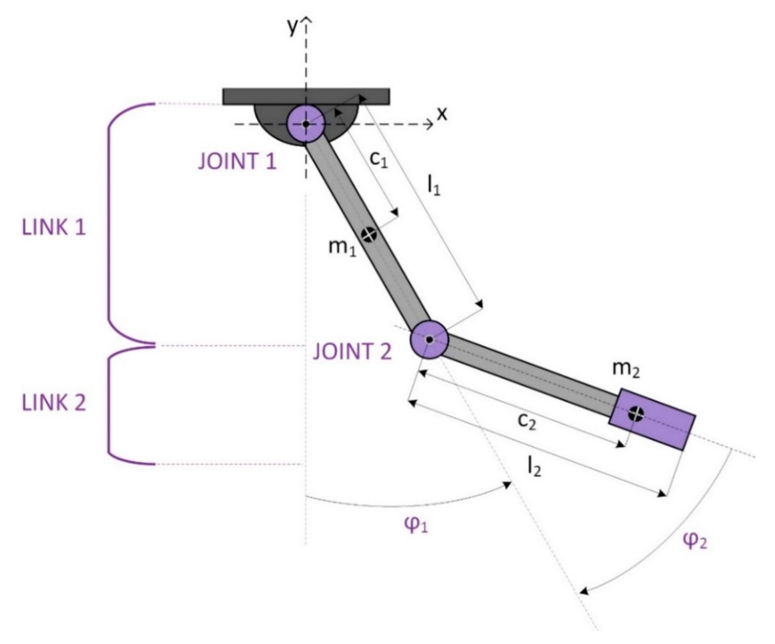
Figure 1. Scheme of kinematic structure of experimental system.
Applsci 11 04490 g001
Figure 2. Experimental system—planar robotic arm with 2-DOF and actuated with PAMs.
Applsci 11 04490 g002
Figure 3. Boxplots of initial values of joint angles—link 1.
Applsci 11 04490 g003
Figure 4. The mean response and standard deviation for the joint angle 10°—link 1.
Applsci 11 04490 g004
Figure 5. The mean response and standard deviation for the joint angle 20°—link 1.
Applsci 11 04490 g005
Figure 6. The mean response and standard deviation for the joint angle 30°—link 1.
Applsci 11 04490 g006
Figure 7. The mean response and standard deviation for the joint angle 40°—link 1.
Applsci 11 04490 g007
Figure 8. The boxplots of initial values of joint angles—link 2.
Applsci 11 04490 g008
Figure 9. The mean response and standard deviation for the joint angle 10°—link 2.
Applsci 11 04490 g009
Figure 10. The mean response and standard deviation for the joint angle 20°—link 2.
Applsci 11 04490 g010
Figure 11. The mean response and standard deviation for the joint angle 30°—link 2.
Applsci 11 04490 g011
Figure 12. The mean response and standard deviation for the joint angle 40°—link 2.
Applsci 11 04490 g012
Figure 13. Model output of validation for the joint angle 10°—link 1.
Applsci 11 04490 g013
Figure 14. Model output of validation for the joint angle 20°—link 1.
Applsci 11 04490 g014
Figure 15. Model output of validation for the joint angle 30°—link 1.
Applsci 11 04490 g015
Figure 16. Model output of validation for the joint angle 40°—link 1.
Applsci 11 04490 g016
Figure 17. Model output of validation for the joint angle 10°—link 2.
Applsci 11 04490 g017
Figure 18. Model output of validation for the joint angle 20°—link 2.
Applsci 11 04490 g018
Figure 19. Model output of validation for the joint angle 30°—link 2.
Applsci 11 04490 g019
Figure 20. Model output of validation for the joint angle 40°—link 2.
Applsci 11 04490 g020
Figure 21. Model output after parameter estimation for the joint angle 10°—link 1.
Applsci 11 04490 g021
Figure 22. Model output after parameter estimation for the joint angle 20°—link 1.
Applsci 11 04490 g022
Figure 23. Model output after parameter estimation for the joint angle 30°—link 1.
Applsci 11 04490 g023
Figure 24. Model output after parameter estimation for the joint angle 40°—link 1.
Applsci 11 04490 g024
Figure 25. Model output after parameter estimation for the joint angle 10°—link 2.
Applsci 11 04490 g025
Figure 26. Model output after parameter estimation for the joint angle 20°—link 2.
Applsci 11 04490 g026
Figure 27. Model output after parameter estimation for the joint angle 30°—link 2.
Applsci 11 04490 g027
Figure 28. Model output after parameter estimation for the joint angle 40°—link 2.
Applsci 11 04490 g028
Figure 29. The best model output before parameter estimation for the joint angle 40°.
Applsci 11 04490 g029
Figure 30. The best model output after parameter estimation for the joint angle 40°.
Applsci 11 04490 g030
Figure 31. Estimation parameters—part 1.
Applsci 11 04490 g031
Figure 32. Estimation parameters—part 2.
Applsci 11 04490 g032
Table 1. The list of main components used in experimental system.
ComponentParameter NameValueComponentParameter NameValue
Fluid muscle
FESTO MAS-20-250N-AA-MC-K
Diameter0.02 mIncremental encoder
KUBLER 3610
Power supply
Max. resolution
5–30 V DC
2500 pulse/rev.
Length0.25 m
Max. muscle force1200 N
Max. working pressure6 bar
Electronic pressure regulator MATRIX EPR50Input signal4–20 mACompressor
FIAC LEONARDO
Max. pressure
Flow
Power
8 bar
105 L/min
750 W
Input pressure1–8 bar
Max. flow60 L/min
Power supply24 V DC
Output pressure0–7 bar
Response60–100 ms
Reaction timeless than 5 ms
Table 2. The list of input parameters of the Simulink model.
NotationDescriptionValue and Unit
m1Mass—link 15.914 kg
m2Mass—link 23.437 kg
l1Length—link 10.615 m
c1Distance to the center of mass—link 10.293 m
c2Distance to the center of mass—link 20.19 m
I1Moment of inertia—link 10.357 kg⋅m2
I2Moment of inertia—link 20.013 kg⋅m2
fc1Viscous friction coefficient—link 10.35 N⋅m⋅s⋅rad−1
fc2Viscous friction coefficient—link 20.35 N⋅m⋅s⋅rad−1
fd1Coulomb friction magnitude—link 10.35 N⋅m
fd2Coulomb friction magnitude—link 20.35 N⋅m
Table 3. Results of validation for link 1.
Angle of RotationMAENRMSE
10°1.093235.47%
20°2.918020.29%
30°3.255034.37%
40°6.171716.69%
Table 4. Results of validation for link 2.
Angle of RotationMAENRMSE
10°0.565514.94%
20°1.107816.36%
30°1.752418.14%
40°2.827016.88%
Table 5. The list of the number of samples and the parameters’ spaces.
Angle of RotationKNotationParameter Estimation Bounds
10°2100m15–7 kg
20°3182m23–5 kg
30°4546l10.5–0.7 m
40°5028c10.2–0.4 m
c20.13–0.25 m
I10.25–0.45 kg⋅m2
I20.009–0.017 kg⋅m2
fc10.00001–20 N⋅m⋅s⋅rad−1
fc20.00001–20 N⋅m⋅s⋅rad−1
fd10.00001–20 N⋅m
fd20.00001–20 N⋅m
Table 6. The list of model parameters after parameter estimation.
NotationValue and UnitNotationValue and Unit
m16.813 kgI10.264 kg⋅m2
m23.361 kgI20.012 kg⋅m2
l10.552 mfc10.335 N⋅m⋅s⋅rad−1
c10.346 mfc20.279 N⋅m⋅s⋅rad−1
c20.212 mfd10.203 N⋅m
fd20.076 N⋅m
Table 7. Results of validation after parameter estimation for link 1.
Angle of RotationMAENRMSE
10°0.607663.96%
20°0.942075.27%
30°1.038281.61%
40°1.104584.62%
Table 8. Results of validation after parameter estimation for link 2.
Angle of RotationMAENRMSE
10°0.240779.64%
20°0.340182.82%
30°0.515981.98%
40°0.720782.69%
Table 9. Comparison of results validation before and after parameter estimation for link 1.
BeforeAfter
Angle of RotationMAENRMSEMAENRMSE
10°1.093235.47%0.607663.96%
20°2.918020.29%0.942075.27%
30°3.255034.37%1.038281.61%
40°6.171716.69%1.104584.62%
Table 10. Comparison of results validation before and after parameter estimation for link 2.
BeforeAfter
Angle of RotationMAENRMSEMAENRMSE
10°0.565514.94%0.240779.64%
20°1.107816.36%0.340182.82%
30°1.752418.14%0.515981.98%
40°2.827016.88%0.720782.69%
Table 11. Comparison of parameters before and after parameter estimation.
NotationValue and Unit
before Estimation
Value and Unit
after Estimation
m15.914 kg6.813 kg
m23.437 kg3.361 kg
l10.615 m0.552 m
c10.293 m0.346 m
c20.19 m0.212 m
I10.357 kg⋅m20.264 kg⋅m2
I20.013 kg⋅m20.012 kg⋅m2
fc10.35 N⋅m⋅s⋅rad−10.335 N⋅m⋅s⋅rad−1
fc20.35 N⋅m⋅s⋅rad−10.279 N⋅m⋅s⋅rad−1
fd10.35 N⋅m0.203 N⋅m
fd20.35 N⋅m0.076 N⋅m
Publisher’s Note: MDPI stays neutral with regard to jurisdictional claims in published maps and institutional affiliations.