Solving Non-Permutation Flow Shop Scheduling Problem with Time Couplings

Abstract

In this paper, a non-permutation variant of the Flow Shop Scheduling Problem with Time Couplings and makespan minimization is considered. Time couplings are defined as machine minimum and maximum idle time allowed. The problem is inspired by the concreting process encountered in industry. The mathematical model of the problem and solution graph representation are presented. Several problem properties are formulated, including the time complexity of the goal function computation and block elimination property. Three solving methods, an exact Branch and Bound algorithm, the Tabu Search metaheuristic, and a baseline Genetic Algorithm metaheuristic, are proposed. Experiments using Taillard-based problem instances are performed. Results show that, for the Tabu Search method, the neighborhood based on the proposed block property outperforms other neighborhoods and the Genetic Algorithm under the same time limit. Moreover, the Tabu Search method provided high quality solutions, with the gap to the optimal solution for the smaller instances not exceeding 2.3%.

1. Introduction

The Flow Shop Scheduling Problem (or FSSP), formulated in both permutation and non-permutation variants [1], remains one of the most well-known optimization problems in operations research. It is widely used for modeling theoretical and real-life problems in manufacturing and production planning [2]. In this problem, a number of jobs and machines are given. The objective is to determine a production schedule such that each job is processed on each machine in the same fixed order (given by the technological process) and the given criterion, usually the completion time of all jobs, is minimized. In the permutation variant, each machine processes jobs in the same order, while non-permutation variant has no such restriction.

Due to its practical applications, a great variety of FSSP variants and extensions have been considered over the years. For example, the authors of [3] considered a cyclic variant, where the initial set of jobs (called Minimal Part Set) is scheduled repeatedly in a cycle with the goal to minimize the cycle time. Another cyclic variant of FSSP, where machines are replaced by single-operator robotic cells, was researched in [4]. Due to the nature of real-life production processes, another common FSSP variant is based on consideration of uncertainty in the data, as shown in [5]. Another FSSP variant, represented by both the previous paper and [6], is multi-criteria FSSP, where two or more optimization criteria are considered simultaneously and the goal is to obtain the Pareto front. For this category of problems, Genetic Algorithms are especially popular recently. For example, the authors in [7] considered a hybrid variant of FSSP, where energy consumption was chosen as an additional objective. Due to a complex nature of the problem, the mixed integer formulation was solved using a modified NSGA-II (Non-dominated Sorting Genetic Algorithm) [8]. A Genetic Algorithm (GA) utilizing the concept of a relative entropy of fuzzy sets was proposed in [9]. To evaluate a Pareto front, the front is first mapped to a fuzzy set and then the relational entropy coefficient is used to measure the similarity to an ideal solution. In experiments for 4, 7, and 10 different criteria, the approach was shown to outperform multiple existing algorithms, including the popular NSGA-III [8,10]. GA approaches are commonly used for solving a wide range of problems ranging from multi-objective train scheduling [11] to continuous process improvement [12].

FSSP is an NP-hard problem and thus considered difficult even for small instances. As a result, there is a great number of different approaches for tackling FSSP. Machine Learning (ML) is a very popular topic nowadays. The methodology is especially well-suited for data-driven problems, with a large volume of noisy information available. However, purely ML-based end-to-end solving methods are usually inferior in the context of classical scheduling and routing problems. For example, the authors in [13] solved Travelling Salesman Problem (TSP) with the Pointer Networks that output a permutation of vertices. However, the approach was strictly worse than the best classical TSP solvers, such as Concorde [14]. Many other authors tried solving TSP using ML methods [15,16], but none succeeded in outperforming the state-of-art. In [17], a more general, data-driven approximation for solving NP-hard problems was presented. The methodology was tested on the Quadratic Assignment Problem. The method was outperformed by a general-purpose commercial solver. On the other hand, ML can also be used as a part of a larger solving algorithm. In a proof-of-concept work [18], the authors proposed an input-size agnostic deep neural network, integrated with Lawler’s decomposition for solving single machine total tardiness problem. The results showed that the algorithm outperformed the former state-of-the-art heuristics and the method can potentially be applied for other problems.

Among classical exact algorithms for FSSP, one can name approaches like Branch and Bound ($\mathrm{B}\&\mathrm{B}$) [19] and Mixed-Integer Linear Programming (MILP) formulations [20]. Heuristic methods include both simpler greedy- or rule-based algorithms [21] and dozens of different metaheuristic algorithms [6,22,23]. Other modeling and solving techniques include the use of fuzzy set theory to represent uncertain data [24] or speeding up computation by the use of parallel computing [25,26]. As reported in of the recent reviews on non-permutation FSSP [2], Genetic Algorithm (GA), Tabu Search (TS), Simulated Annealing, and Ant Colony Optimization are the most popular metaheuristic algorithms for FSSP. As noted earlier, GA has been used recently to solve many multi-criteria variants FSSP. However, the algorithm is also well-suited for a single-objective FSSP. For example, in [27], GA was used to solve a variant of a hybrid FSSP with unrelated machines, machine eligibility, and total tardiness minimization. The authors incorporated a new decoding method tuned for the specific objective function considered. The resulting algorithm proved to be competitive in numerical experiments. The authors in [28] considered a permutational FSSP with flow time minimization. A Biased Random-Key Genetic Algorithm was proposed, introducing a new feature called shaking. Authors compared the results obtained by their algorithms with an Iterated Greedy Search, an Iterated Local Search, and a commercial solver. Variants of the proposed algorithm outperformed the competition, especially for larger instances.

Despite a large variety of extensions, the existing variants of FSSP are often insufficient in practice, when considering problems with machines that have unusual characteristics. Our motivation and an example of such problem is the concreting process, where one of the tasks performed on the site is concrete mix pouring. The concrete mixer needs to load the next batch of the mixture before proceeding with the next site. Moreover, the mixture has to be mixed for appropriate time before pouring—too long or too short mixing can affect the properties of the mixture or even damage the vehicle. However, the mixing should not be included in task time because work on the site can proceed as soon as the concrete mixer leaves the site. In scheduling, we can describe this as an additional dependency between starting or completion times of operations within a single machine (the concrete mixer in our case). As a result, additional gaps of minimum and maximum allowed lengths are inserted into the schedule. We will refer to such restrictions as time couplings and to FSSP with those restrictions as Flow Shop Scheduling Problem with Time Couplings (or FSSP-TC).

The minimal waiting time needed for the concrete mixing can be modeled as a setup time [22], but this does not model the maximal waiting time. Other similar time constraints found in the literature include a classic no-idle [29,30], where each machine, once processing operations are started, cannot be idle until all its operations are completed. Setups and no-idle constraints together were considered in [31], where subsequent operations or setups must start immediately after previous ones have completed. The authors proposed an MILP formulation as well as several versions of a heuristic based on the Beam Search approach.

Similarly to no-idle, a no-wait constraint describes a requirement whose next operation in a job has to be started directly after completing the previous one. An example of such constraint for FSSP was considered in [32] and solved through various local-search metaheuristics. In [33], the authors proposed an application of genetic operators to an Ant Colony Optimization algorithm for the same variant of FSSP. The described algorithm was applied to the 192 benchmark instances from literature. Results were compared with an Adaptive Learning Approach and Genetic Heuristic algorithm. The authors in [34] considered an energy-efficient no-wait permutation FSSP with makespan and energy consumption minimization. To achieve a better energy utilization, the processing speeds of machines can be dynamically adjusted for different jobs, altering both processing times and energy consumption. To solve the multi-criteria optimization problem, an adaptive multi-objective Variable Neighborhood Search algorithm was proposed, outperforming several state-of-art evolutionary algorithms. A modification of a classic no-wait, a limited wait constraint, in the context of a hybrid FSSP, was considered in [35]. A limited wait occurs, when some types of products (jobs) can wait for being processed at the next machine, and some cannot. The problem was solved by a discrete Particle Swam Optimization algorithm. In [36], a two-machine FSSP with both no-idle and no-wait constraints considered simultaneously was researched. Authors proposed a metaheuristic algorithm, utilizing Integer Linear Programming formulation. The method was able to obtain competitive results for instances consisting of up to 500 jobs. Another example of time constraints is minimum-maximum time allowed between consecutive operations of a single job. A two-machine FSSP with such constraints was researched in [20], where some theoretical proprieties of the problem were proven.

Nevertheless, none of the mentioned problems can precisely model the aforementioned concreting process. An adequate model was shown in [37], along with $\mathrm{B}\&\mathrm{B}$ and TS solving methods. However, the authors considered only the permutation variant of FSSP-TC and did not propose any elimination properties. We aim to rectify those drawbacks. Thus, our contributions can be summarized as:

• Formulation of the mathematical model for the concreting process.
• Identification of several problem properties, including elimination blocks.
• Proposal of three solving algorithms for the considered problem: B&B, TS, and GA, out of which TS utilizes the proposed block properties.

The remainder of the paper is organized as follows: in Section 2, a formal mathematical model of the problem is formulated, along with a graph representation. Next, in Section 3, several problem properties are proven, including the elimination (block) property. Then, solving algorithms are presented in Section 4. The algorithms are empirically evaluated in Section 5. The paper is concluded in Section 6.

2. Problem Formulation

In this section, we will formulate the FSSP-TC formally, including the notation, problem constraints, and the goal function. The formulation is based on the classic FSSP, intended as an extension.

2.1. Mathematical Model

Let $\mathcal{J}=\{1,2,\dots ,n\}$ and $\mathcal{M}=\{1,2,\dots ,m\}$ be sets of n jobs and m machines, respectively. Each job j is composed of m operations from the set ${\mathcal{O}}_j=\{l_j+1,l_j+2,\dots ,l_j+m\}$, where $l_j=m(j-1)$. Thus, there are $nm$ operations in total and sets ${\mathcal{O}}_j$ partition set $\mathcal{O}$—the set of all operations. Each job j has to be processed on the machines in the natural order: $1\to 2\to \cdots \to m$. The processing time of job j on machine i (i.e., operation $l_j+i$) is denoted $p_{i,j}>0$. Moreover, let ${\widehat{r}}_i\ge 0$ denote the minimum idle time machine i is allowed between the processing of subsequent operations. Similarly, ${\widehat{d}}_i\ge {\widehat{r}}_i$ denotes the maximum idle time.

While the order in which jobs are processed is fixed, the processing order for each machine is a decision variable. Let ${\pi }_i$ be an n-element sequence of jobs that are to be processed on machine i, such that ${\pi }_i\left(j\right)$ is the j-th job to be processed on i. Then, the overall processing order is given by sequence $\pi =({\pi }_1,{\pi }_2,\dots ,{\pi }_m)$. Sequence $\pi$ will be called a solution. Based on solution $\pi$, one can build a corresponding schedule. The schedule $(S,C)$ consists of two matrices. The first matrix is given by $S={\left[S_{i,j}\right]}^{m\times n}$, where $S_{i,j}$ is the starting time of the j-th operation to be processed on machine i in $\pi$. Similarly, we can define the matrix of operation completion times $C={\left[C_{i,j}\right]}^{m\times n}$, where element $C_{i,j}$ is the completion time of j-th operation to be processed on machine i according to $\pi$. For a schedule $(S,C)$ to be feasible, it needs to meet the following constraints:

$$\begin{array}{cc}\hfill \forall i\in \mathcal{M}\hspace{1em}\forall j\in \mathcal{J}& C_{i,j}=S_{i,j}+{\rho }_{i,j},\hfill \end{array}$$

(1)

$$\begin{array}{cc}\hfill \forall i\in \mathcal{M}\hspace{1em}\forall j\in \mathcal{J}\setminus \left\{1\right\}& {\widehat{r}}_i\le S_{i,j}-C_{i,j-1}\le {\widehat{d}}_i,\hfill \end{array}$$

(2)

$$\begin{array}{cc}\hfill \forall i\in \mathcal{M}\setminus \left\{1\right\}\hspace{1em}\forall j\in \mathcal{J}& S_{i,j}\ge C_{i-1,{\pi }_{i-1}^{-1}\left({\pi }_i\left(j\right)\right)},\hfill \end{array}$$

(3)

where ${\rho }_{i,j}$ is a shorthand for $p_{i,{\pi }_i\left(j\right)}$, and ${\pi }_i^{-1}\left(j\right)$ is the position of job j in ${\pi }_i$ (i.e., ${\pi }_i^{-1}\left(k\right)=j\iff {\pi }_i\left(j\right)=k$). In other words, ${\pi }^{-1}$ is inversion of permutation $\pi$. We also assume, without losing generality, that the first operation on the first machine starts at time 0, resulting in $S_{1,1}=0$.

Constraint (1) means the processing of operations cannot be interrupted. Constraint (2) enforces that minimum and maximum machine idle times are respected, but also requires that operation a on machine i is only started after previous operation on i (i.e., machine predecessor of a) has completed. Similarly, (3) ensures that operation a of job j is started only after previous operation of job j (i.e., the technological predecessor of a) has completed.

From (1), one can observe that a feasible schedule can be described unambiguously by either S or C, which will be used throughout the paper. A schedule is called left-shifted if no operations can start sooner without violating the constraints or changing the processing order. A method for computing a left-shifted schedule S from a solution $\pi$ will be presented in Section 3.

Example 1.

Consider the FSSP instance from

Table 1. Problem instance from Example 1 for $n=5$ and $m=3$.

a	${\mathit{p}}_{\mathit{a},1}$	${\mathit{p}}_{\mathit{a},2}$	${\mathit{p}}_{\mathit{a},3}$	${\mathit{p}}_{\mathit{a},4}$	${\mathit{p}}_{\mathit{a},5}$	${\widehat{\mathit{r}}}_{\mathit{a}}$	${\widehat{\mathit{d}}}_{\mathit{a}}$
1	2	1	2	1	3	1	5
2	1	2	1	2	1	1	2
3	2	2	3	2	1	0	0

for $n=5$, $m=3$ and order of jobs $\pi =\left(\right(2,5,4,3,1),\hspace{1em}(2,4,5,1,3),\hspace{1em}(4,5,2,1,3\left)\right)$. A left-shifted schedule for solution π, with $C_{\max }=27$, is shown as a Gantt chart in Figure 1. Note that π is not optimal, as any change in ${\pi }_3$ will result in a smaller makespan.

Finally, we will define the goal function to be optimized. Let $C_{\max }\left(\pi \right)$ be the completion time of the operation that completes last in the left-shifted schedule corresponding to $\pi$. From constraints (1)–(3), it follows that $C_{\max }\left(\pi \right)=C_{m,n}$. The goal is to find a solution ${\pi }^{*}$, such that

$$C_{\max }\left({\pi }^{*}\right)=\underset{\pi \in \mathsf{\Pi }}{min}{C}_{\max }\left(\pi \right),$$

(4)

where $\mathsf{\Pi }$ is the set of all feasible solutions. The solution ${\pi }^{*}$ is called the optimal solution. In Graham notation, we will denote this problem as $F|{\widehat{r}}_i,{\widehat{d}}_i|C_{\max }$.

We will also consider several special cases of the $F|{\widehat{r}}_i,{\widehat{d}}_i|C_{\max }$ problem. When ${\widehat{d}}_i=0$ (for all i), we obtain the classic no-idle constraint, i.e., the $F\left|\mathrm{no}-\mathrm{idle}\right|C_{\max }$ problem. When ${\widehat{d}}_i=\infty$, we have only the minimum idle time constraint, denoted as $F|{\widehat{r}}_i|C_{\max }$. When ${\widehat{r}}_i=0$, we have only the maximum idle time, denoted by $F|{\widehat{d}}_i|C_{\max }$. Finally, when both ${\widehat{r}}_i=0$ and ${\widehat{d}}_i=\infty$, then we obtain the classic FSSP, i.e., $F\left|\right|C_{\max }$. It should be noted that the results from this paper can be applied to any of those special cases, especially for $F|{\widehat{d}}_i|C_{\max }$ and $F|{\widehat{r}}_i|C_{\max }$, for which more specific approaches are not yet formulated.

2.2. Graph Model

One of the classical techniques in scheduling is representing a problem instance (or a solution) as a graph. For Flow Shop problems, both approaches are widely used in a form of disjunctive [38] and solution graphs [39]. The latter can be used e.g., to check solution feasibility or for the goal function evaluation purpose [40]. In this subsection, we will introduce graph $G\left(\pi \right)$, constructed for solution $\pi$.

First, let us introduce a solution graph for a classical, non-permutation FSSP, given by $G^{\prime }\left(\pi \right)=(V,E_1\cup E_2)$, where

$$\begin{array}{cc}\hfill V& =\bigcup _{\begin{array}{c}i\in \mathcal{M}\\ j\in \mathcal{J}\end{array}}\left\{(i,j)\right\},\hfill \end{array}$$

(5)

$$\begin{array}{cc}\hfill E_1& =\bigcup _{\begin{array}{c}i\in \mathcal{M}\\ j\in \mathcal{J}\setminus \left\{1\right\}\end{array}}\left\{\left((i,j-1),(i,j)\right)\right\},E_2=\bigcup _{\begin{array}{c}i\in \mathcal{M}\setminus \left\{1\right\}\\ j\in \mathcal{J}\end{array}}\left\{\left((i-1,I_{i-1}\left({\pi }_i\left(j\right)\right)),(i,j)\right)\right\}.\hfill \end{array}$$

(6)

The vertices in V represent operations and will be placed on a grid for an easier visualization. The operation of job j on machine i will be represented by a weighted vertex in j-th “column” and i-th “row”, denoted by $(i,j)$ and with weight ${\rho }_{i,j}$. The arcs of graph $G^{\prime }\left(\pi \right)$ are weightless and represent problem constraints ($E_1$ represents machine constraints, and $E_2$—technological constraints). Finally, the length of the longest path to vertex $(i,j)$ equals $C_{i,j}$. Length of the path is defined in this paper as a sum of weights of its vertices and arcs. Thus, the value of the makespan $C_{\max }\left(\pi \right)$ is equal to the length of the longest path in the graph $G^{\prime }\left(\pi \right)$ (critical path). We denote length of a path c by $\mathrm{len}\left(c\right)$.

We will now move onto extended graph $G\left(\pi \right)$. To reflect minimum idle times in the graph, we will use the same technique as for setup times [40]. Each arc $\left(\right(i,j),(i,j+1\left)\right)$ in $E_1$ now has a weight of ${\widehat{r}}_i$. Secondly, we will introduce another set of arcs, to reflect maximum idle time [37]

$$E_3=\bigcup _{i\in \mathcal{M}}\bigcup _{j\in \mathcal{J}\setminus \left\{n\right\}}\left\{\left((i,j+1),(i,j)\right)\right\}.$$

(7)

Any “return” arc $\left(\right(i,j+1),(i,j\left)\right)$ in $E_3$, has weight ${\widehat{D}}_{i,j}$, defined as

$${\widehat{D}}_{i,j}=-{\rho }_{i,j}-{\rho }_{i,j+1}-{\widehat{d}}_i.$$

(8)

A structure of graph $G\left(\pi \right)$ for the solution $\pi$ from Example 1 is shown in Figure 2. For more readability, arcs from sets $E_1$, $E_2$ and $E_3$ are marked in green solid, blue dashed, and red dotted lines, respectively:

3. Problem Properties

In this section, we will discuss several properties for the $F|{\widehat{r}}_i,{\widehat{d}}_i|C_{\max }$ problem including: feasibility of solutions, computational complexity of determining the goal function, and an elimination property based on blocks.

Property 1.

For any solution $\pi \in \mathsf{\Pi }$, the solution graph $G\left(\pi \right)$ for $F|{\widehat{r}}_i,{\widehat{d}}_i|C_{\max }$ does not contain cycles of positive length.

Proof. 

Let us notice that graph $G\left(\pi \right)$ does not contain arcs going “upwards” (i.e., no arcs from vertex $(i,j)$ to $(k,j)$ for $k<i$). Thus, cycles can only be created with the use of “horizontal” arcs.

Let us consider a cycle consisting of two adjacent vertices $(i,j)$ and $(i,j+1)$. Those vertices have weights ${\rho }_{i,j}$ and ${\rho }_{i,j+1}$, while the arcs connecting them have weights ${\widehat{r}}_j$ and ${\widehat{D}}_{i,j}=-{\rho }_{i,j}-{\rho }_{i,j+1}-{\widehat{d}}_i$. After adding the weights together, the length of such a cycle is equal to ${\widehat{r}}_j-{\widehat{d}}_i\le 0$.

Now, let us generalize this result to cycles consisting of $k>2$ subsequent vertices in one “row”. Such a cycle contains (for some i and j) vertices from $(i,j)$ to $(i,j+k-1)$, as well as $k-1$ “forward” arcs with weights ${\widehat{r}}_j$ and $k-1$ “return” arcs. Let us now compute the length of such a cycle. Without loss of generality, we can assume that the cycle begins in vertex $(i,j+k-1)$. Let us consider the inner vertices of this cycle i.e., vertices from $(i,j+1)$ to $(i,j+k-2)$. Let $(i,c)$ denote one such inner vertex. We pass each vertex $(i,c)$ twice during the cycle, thus adding weight $2{\rho }_{i,c}$ to the cycle length. Moreover, when passing through vertex $(i,c)$, we add the weight $-{\rho }_{i,c}$ twice: once from “return” arc ending at $(i,c)$ and once from “return” arc starting at $(i,c)$. Thus, so far, the cycle length is 0, as all weights $2{\rho }_{i,c}$ and $-2{\rho }_{i,c}$ add up to 0.

The above is thus equal to a situation where vertices $(i,j+1)$ to $(i,j+k-2)$ have weights 0 and “return” arcs have only term ${\widehat{d}}_i$ in their weight. The only exceptions are the “return” arc starting at vertex $(i,j+k-1)$ and the “return” arc ending at vertex $(i,j)$. Those two arcs still have the terms $-{\rho }_{i,j+k-1}$ and $-{\rho }_{i,j}$ in their weights, respectively. However, it is easy to see that those two terms will be negated by the weights of vertices $(i,j)$ and $(i,j+k-1)$ as we pass those vertices only once during the cycle. Thus, we can compute the cycle length as if all cycle vertices had weights 0 and its “return” arcs had weights with term ${\widehat{d}}_i$ only. The cycle length is then $(k-1)({\widehat{r}}_i-{\widehat{d}}_i)\le 0$. □

Therefore, all cycles in $G\left(\pi \right)$ are of non-positive length. When computing the value of the makespan, we can ignore those cycles as per the following observation.

Corollary 1.

For any solution π, if solution graph $G\left(\pi \right)$ for the $F|{\widehat{r}}_i,{\widehat{d}}_i|C_{\max }$ problem contains a path p with length $\mathrm{len}\left(p\right)$ such that p contains a cycle, then $G\left(\pi \right)$ also contains a path P without a cycle, such that:

$$\mathrm{len}\left(P\right)\ge \mathrm{len}\left(p\right).$$

(9)

Thus, if a path p in $G\left(\pi \right)$ contains a cycle, then either: (1) it is not the longest path in $G\left(\pi \right)$ (at least one cycle in p has negative length) or (2) we can construct another path starting and ending at the same vertices and with the same length as p, but not containing a cycle (all cycles in p have length 0).

We will now present the algorithm for determining the left-shifted feasible schedule S (and thus the makespan $C_{\max }$), based on the solution $\pi$. We will also provide the computational complexity of this algorithm.

Theorem 1.

For any solution π, there exists a feasible left-shifted schedule S for the $F|{\widehat{r}}_i,{\widehat{d}}_i|C_{\max }$ problem. Moreover, the value $C_{\max }\left(\pi \right)$ for the schedule S can be determined in time $O\left(nm\right)$.

Proof. 

The proof is based on Algorithm 1. Here, we will describe it, including its computational complexity. The algorithm consists of m phases. In phase i, we determine the completion times for all operations on machine i. Every time a completion time $C_{i,j}$ is computed or updated, we also set $S_{i,j}=C_{i,j}-{\rho }_{i,j}$. By doing so, we met the constraint (1) at all times throughout the algorithm.

Algorithm 1: Constructing left-shifted schedule.

Phase 1 corresponds to lines 1–3 of the algorithm. In line 1, we set $C_{i,j}={\rho }_{1,1}$, since the first operation on the first machine has no constraints. Then, in lines 2 and 3, we set completion times for subsequent remaining operations on this machine. Constraints (2) and (3) for this machine will be met because ${\widehat{d}}_1\ge {\widehat{r}}_1$ and operations on machine 1 have no technological predecessors. The schedule on machine 1 is thus set, feasible and left-shifted, as scheduling any operation earlier would violate either the left side of constraint (2) or make $S_{1,1}$ a negative number. From the pseudocode, it is also easy to see that this phase is computed in time $O\left(n\right)$.

Let us now consider phases $i>1$ (lines 4 to 9). We always complete phase i before starting phase $i+1$ (line 4). Each such phase is executed in a similar manner. First, in line 5, we tentatively set $C_{i,1}$, similarly to line 1, except we also consider the technological predecessor of that operation. Then, in lines 6–7, we tentatively set completion times of subsequent operations, taking into account technological predecessor, machine predecessor, and minimal idle time ${\widehat{r}}_i$.

By now, the only constraint operations on machine i might still violate is the right side of constraint (2). In order to mitigate that, in lines 8–9, we perform similar operation to lines 6–7, but in reverse order (from operation $n-1$ down to 1). In particular, if $C_{i,j}$ and $C_{i,j+1}$ are such that the right side of constraint (2) is violated, then we shift $C_{i,j}$ to the right just enough to meet the constraint, after which the value of $C_{i,j}$ is final. During this procedure, some of the operations might be rescheduled to start later, thus this change will not violate any constraints. Moreover, now the constraint (2) is guaranteed to hold.

The schedule on machine i is thus feasible and left-shifted. Indeed, if no operation was shifted to be scheduled later during the correction procedure, then we cannot shift any operation to schedule earlier because this would violate either the left side of constraint (2) or constraint (3). Similarly, if an operation was shifted during the correction, then the shift was the smallest that met the right side of constraint (2). Any smaller shift would create infeasible schedule, so shifting the operation to start any earlier is not possible.

We also see from the pseudocode that each phase $i>1$ can by completed in time $O\left(n\right)$. Thus, all m phases can be computed in time $O\left(nm\right)$, allowing us to obtain a feasible left-shifted schedule for any $\pi$ with $C_{\max }=C_{m,n}$. □

From the above theorem, it follows that all solutions $\pi$ are feasible. However, we will show that some of the feasible solutions can be disregarded. Particularly, many solving methods use the concept of a move. For example, we can define the swap move for the $F|{\widehat{r}}_i,{\widehat{d}}_i|C_{\max }$ problem as follows:

$${\pi }^{\prime }=\mathrm{swap}(\pi ,i,j,k),$$

(10)

where solution ${\pi }^{\prime }$ is created from $\pi$ by swapping together values of ${\pi }_i\left(j\right)$ and ${\pi }_i\left(k\right)$. The solution ${\pi }^{\prime }$ will be called the neighbor of solution $\pi$. Similarly, the set of all solutions created from $\pi$ by this move will be called the neighborhood of $\pi$.

We will now formulate an elimination property showing that some moves do not result in immediate improvement of the makespan, similarly to existing elimination properties for the Job Shop Scheduling problem [41]. Let us start with the definition of a block. A sequence of operations $B=(b_1,b_2,\cdots ,b_c)$ for $c>0$ will be called a block if and only if:

• All operations from B are on the same critical path.
• Operations from B are performed subsequently on the same machine i.
• Operations from B are processed on i in the order of their appearance in B.
• The length of B is maximum i.e., operations from i that are directly before or after B cannot be included in it without violating the first three conditions.

Moreover, for block $B=(b_1,b_2,b_3,\cdots ,b_{c-2},b_{c-1},b_c)$ of $c>2$ operations, we define its inner block as sequence $B^{\prime }=(b_2,b_3,\cdots ,b_{c-2},b_{c-1})$.

Let block $B=(b_1,b_2,\dots ,b_c)$ be part of critical path K. Then, B is called a right-side block (or R-block) if the first operation from B on K is $b_1$. Similarly, B will be called a left-side block (or L-block) if the first operation from B on K is $b_c$.

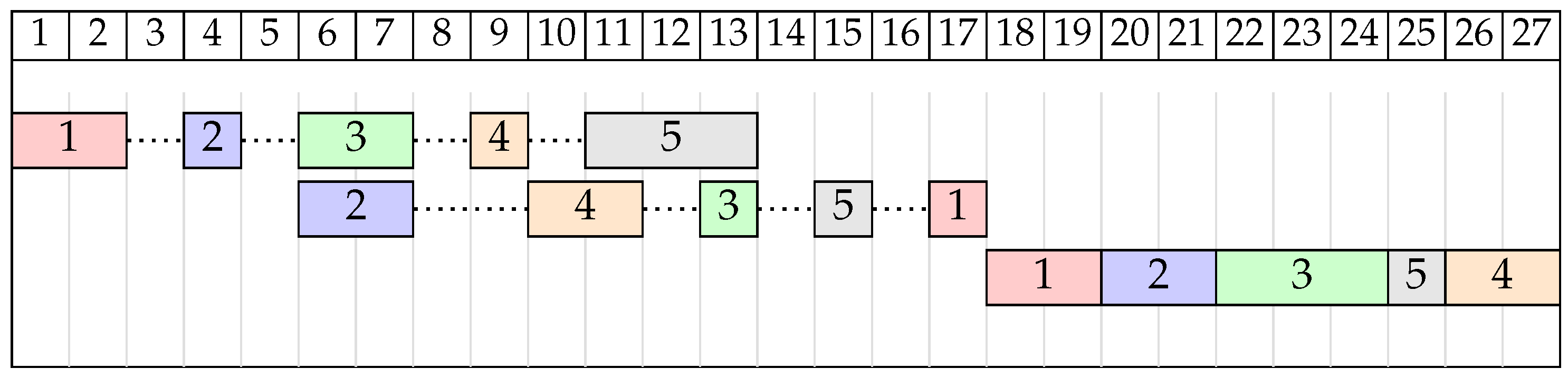
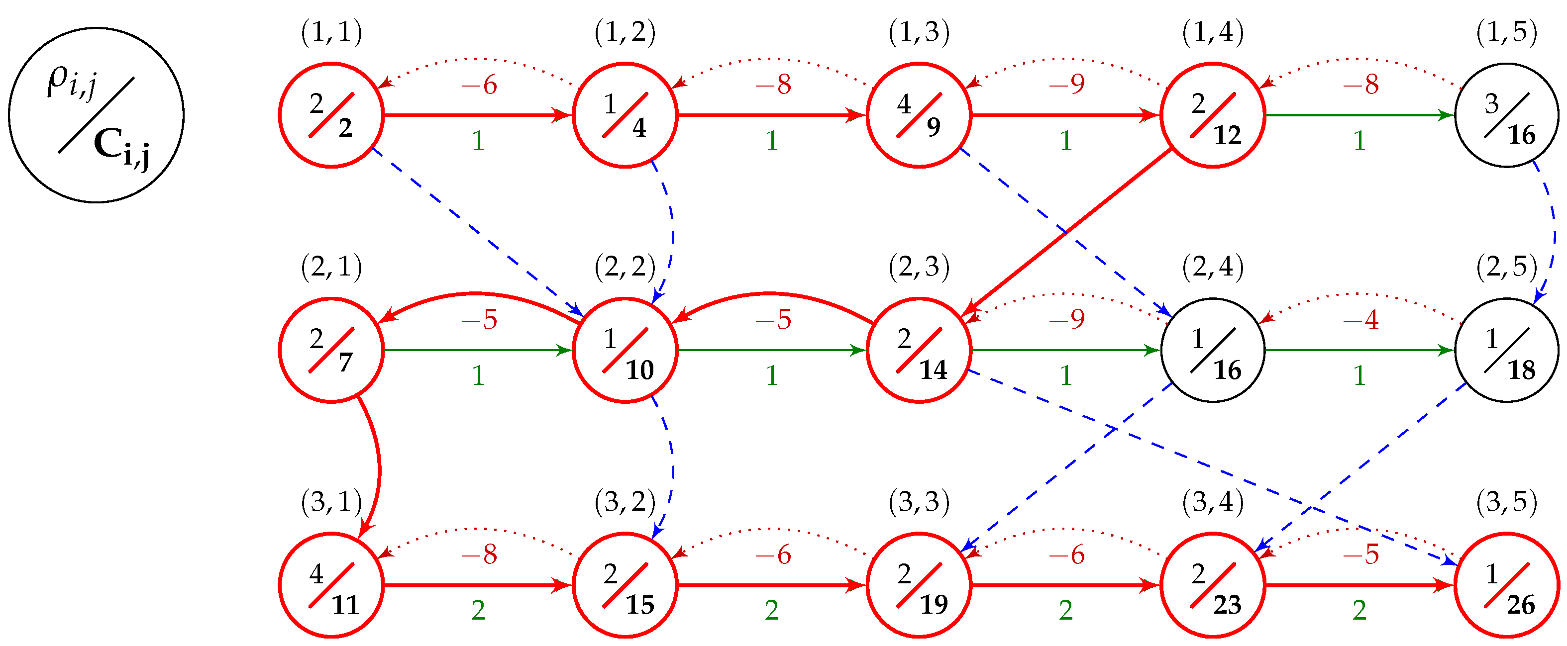
Example 2.

Consider the FSSP instance for $n=5$, $m=3$ from

Table 2. Problem instance from Example 2 for $n=5$ and $m=3$.

a	${\mathit{p}}_{\mathit{a},1}$	${\mathit{p}}_{\mathit{a},2}$	${\mathit{p}}_{\mathit{a},3}$	${\mathit{p}}_{\mathit{a},4}$	${\mathit{p}}_{\mathit{a},5}$	${\widehat{\mathit{r}}}_{\mathit{a}}$	${\widehat{\mathit{d}}}_{\mathit{a}}$
1	2	1	4	2	3	1	3
2	1	2	1	2	1	1	2
3	2	4	2	1	2	2	2

. Let us assume the order of jobs $\pi =({(1,2,3,4,5)}_{,} (2,1,4,3,5), (2,1,3,5,4))$. Solution graph $G\left(\pi \right)$ for this example is shown in Figure 3 with the critical path shown in bolded red. This critical path is composed of three blocks (one for each machine). On the first machine, we have a 4-operation R-block beginning at operation $(1,1)$ and ending at operation $(1,4)$. On the second machine, we have an L-block of size 3 starting at operation $(2,3)$ and going back to operation $(2,1)$. Finally, on the last machine, we again have an R-block which runs through all five operations of that machine. Let us also note that the sizes of the inner blocks are 2, 1, and 3, respectively. The left-shifted schedule for solution π, with $C_{\max }=26$, is shown as a Gantt chart in Figure 4.

With the concept of blocks and inner blocks defined, we can formulate the block elimination property for the $F|{\widehat{r}}_i,{\widehat{d}}_i|C_{\max }$ problem.

Theorem 2.

Let $\pi =({\pi }_1,{\pi }_2,\cdots ,{\pi }_m)$ be a solution to the $F|{\widehat{r}}_i,{\widehat{d}}_i|C_{\max }$ problem and let $B=(b_1,b_2,\cdots ,b_c)$, $c>2$ be a block on a critical path K in $G\left(\pi \right)$ consisting of operations from machine i. Next, let ${\pi }^{\prime }$ be a solution created from π by swapping any pair of operation from inner block of B i.e.,:

$${\pi }^{\prime }=\mathrm{swap}(i,j,k)j,k\in \{b_2,b_3,\dots ,b_{c-2},b_{c-1}\}, j\ne k,$$

(11)

then:

$$C_{\max }\left({\pi }^{\prime }\right)\ge C_{\max }\left(\pi \right).$$

(12)

Proof. 

Due to Property 1 and Corollary 1, there is at least one cycle-free critical path that contains the block B. We arbitrarily choose one of such paths to be our critical path K.

It follows that the critical path travels through block B in one direction (the critical path does not change direction in the middle of B). Thus, B is either an L-block or an R-block and we need to prove the elimination property for both types of blocks.

Let us notice that the “downwards” arc entering B from the previous machine (if $i>1$) always enters B either at the beginning (at operation $b_1$) or at the end (at operation $b_c$) of B, making the B and R- and L-block, respectively. The same happens for the arc exiting the block “downwards” onto the next machine (for $i<m$): that arc exits from $b_1$ for an L-block and and from $b_c$ for an R-block.

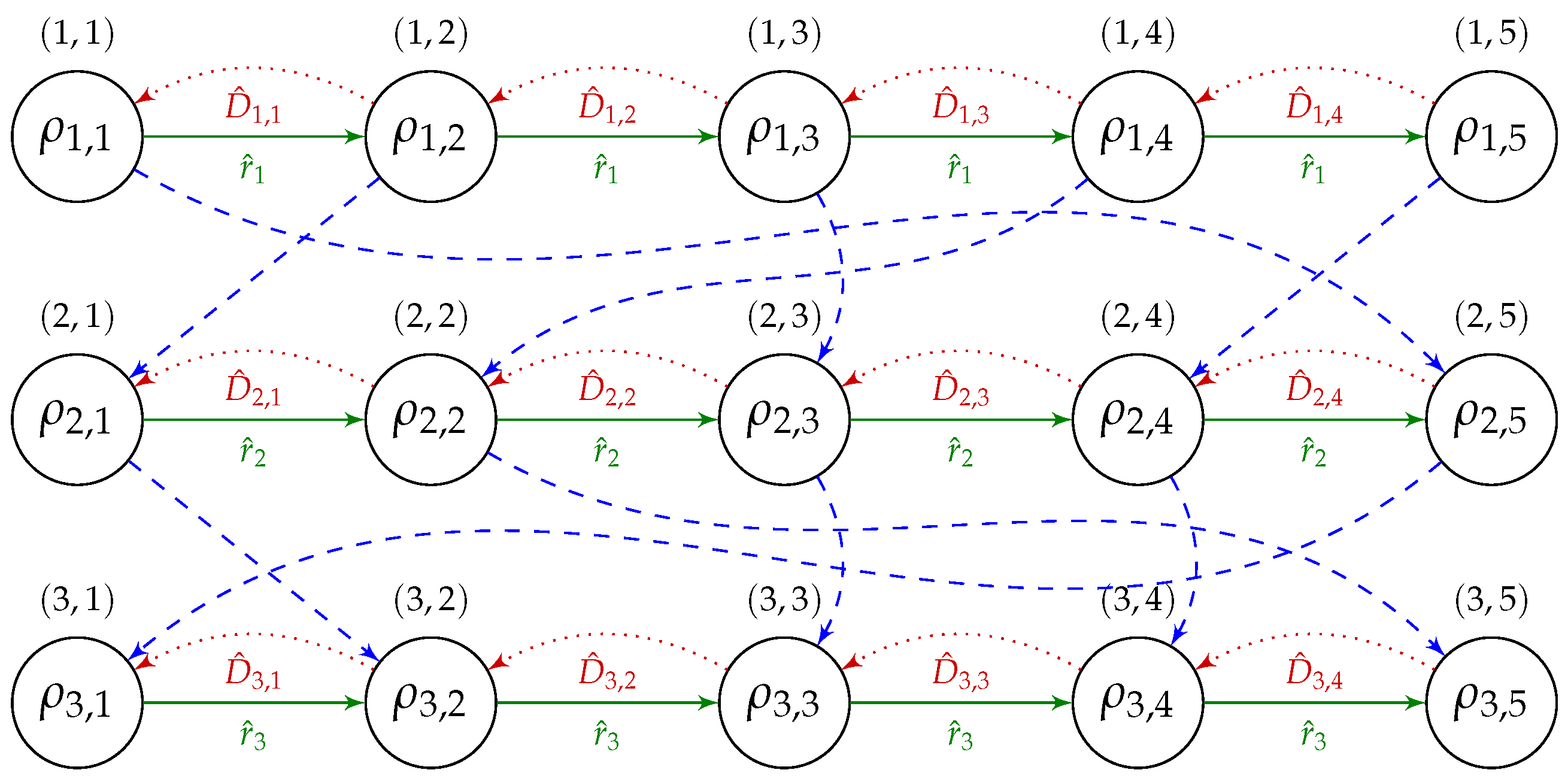
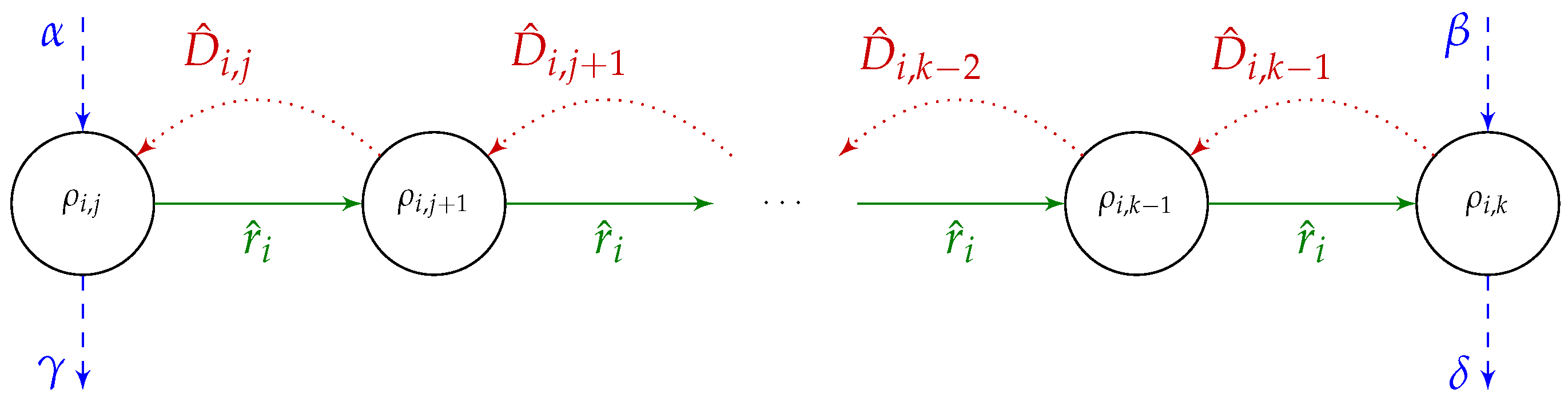
Let us assume that operations $(b_1,b_2,\dots ,b_c)$ of B are operations from jobs $j,j+1,\dots ,k-1,k$, respectively. Let $\alpha$ and $\gamma$ be the lengths of the longest paths ending and starting at vertex $(i,j)$, without the weight of that vertex. Similarly, let $\beta$ and $\delta$ be the lengths of the longest path ending and starting at vertex $(i,k)$ without the weight of that vertex. The relevant part of graph $G\left(\pi \right)$, including block B and paths $\alpha$, $\beta$, $\gamma$ and $\delta$ is shown in Figure 5.

Let us start with the R-block case. The length of the critical path will be:

$$\alpha +{\rho }_{i,j}+{\rho }_{i,j+1}+\cdots +{\rho }_{i,k-1}+{\rho }_{i,k}+{\widehat{r}}_i(k-j){\widehat{r}}_i+\delta .$$

(13)

The inner block for B is $B^{\prime }=(b_2,b_3,\dots ,b_{c-1})$. Now, let us consider swapping any two operations $b_x,b_y\in B^{\prime }$, with $x\ne y$. Such a swap will not affect the lengths of paths $\alpha$ and $\delta$. It will also not change values ${\rho }_{i,j}$ and ${\rho }_{i,k}$, as vertices $(i,j)$ and $(i,k)$ are outside of the inner block. Values ${\widehat{r}}_i$ are unaffected as well. The swap of operations $b_x$ and $b_y$ will change the order of the values ${\rho }_{i,j+1}$ through ${\rho }_{i,k-1}$, but their sum will remain unchanged. The length of the considered critical path will thus remain the same. Thus, graph $G\left({\pi }^{\prime }\right)$ will contain a path with the length at least as large as the length of path K in $G\left(\pi \right)$ and in conclusion:

$$C_{\max }\left({\pi }^{\prime }\right)\ge C_{\max }\left(\pi \right).$$

(14)

Now, let us consider the L-block case. The length of the critical path is then:

$$\beta +{\rho }_{i,j}+{\rho }_{i,j+1}+\cdots +{\rho }_{i,k-1}+{\rho }_{i,k}+{\widehat{D}}_{i,j}+{\widehat{D}}_{i,j+1}+\cdots +{\widehat{D}}_{i,k-1}+\gamma .$$

(15)

Once again, we consider swapping operations $b_x$ and $b_y$ from inner block of B. The length of paths $\beta$ and $\gamma$ does not change, similar to weights of vertices $(i,j)$ and $(i,k)$ because they are outside the inner block. The swapping of $b_x$ and $b_y$ will also not affect the sum of weights of vertices $(i,j+1)$ to $(i,k-1)$ as they will all still be a part of the inner block after the swap, just in a different order.

All that is left to consider are the arc weights ${\widehat{D}}_{i,j}$ through ${\widehat{D}}_{i,k-1}$. Part of those weights are the ${\widehat{d}}_i$ terms which will not change as they are independent from solution $\pi$ (or ${\pi }^{\prime }$). Values ${\rho }_{i,j}$ and ${\rho }_{i,k}$ that are part of weights ${\widehat{D}}_{i,j}$ and ${\widehat{D}}_{i,k-1}$ will not change because they are dependent on weights of vertices $(i,j)$ and $(i,k)$, which were unaffected by the swap. The last remaining contribution to weights ${\widehat{D}}_{i,z}$ for z from j through $k-1$ are the values $-{\rho }_{i,z}$ and $-{\rho }_{i,z+1}$. Those values are dependent on vertex $(i,z)$ and its weight of ${\rho }_{i,z}$. However, we know that all weights ${\rho }_{i,z}$ will remain in the inner block (just changing their order). Thus, the operation swap will not change their total contribution into weights ${\widehat{D}}_{i,z}$, and the final sum of weights ${\widehat{D}}_{i,j}$ through ${\widehat{D}}_{i,k-1}$ does not change.

As a result, the graph $G\left({\pi }^{\prime }\right)$ will contain a path of the length the same as critical path K in $G\left(\pi \right)$, thus:

$$C_{\max }\left({\pi }^{\prime }\right)\ge C_{\max }\left(\pi \right).$$

(16)

 □

The above theorem proves that the swapping of operations in an inner block will not result in an immediate improvement of $C_{\max }$. It is similar for the swapping of operations outside of the block (they lie outside of the critical path). Thus, the most promising option is to perform a swapping move where one operation is from the inner block and one is outside of it.

4. Solving Methods

In this section, we will propose three methods for solving the $F|{\widehat{r}}_i,{\widehat{d}}_i|C_{\max }$ problem: a Branch and Bound ($\mathrm{B}\&\mathrm{B}$) method, as well as Tabu Search (TS) and Genetic Algorithm (GA) metaheuristics. Due to its ability to obtain an optimal solution, the B&B method will be used as a reference for evaluating the quality of the TS method for smaller instances. Similarly, GA will serve as a baseline comparison to TS for larger instances.

4.1. Branch and Bound

Branch and Bound ($\mathrm{B}\&\mathrm{B}$) [19] is an exact method using lower and upper bounds to skip parts of the solution space that cannot contain the optimal solution. Our implementation is based on a priority queue $\mathcal{Q}$ of nodes. Each queue element $\nu$ contains a partial solution (${\nu }_{\pi }$), the machine on which a current algorithm branch is executing (${\nu }_{\mathrm{L}}$), a set ${\nu }_{\mathrm{N}}$ of jobs not yet scheduled on this machine, and the lower bound $LB\left(\nu \right)$.

The branching method is similar to the one used for the Job Shop Scheduling Problem [42]: first, we consider all jobs on the current permutation level before proceeding to the next one, avoiding having to process the same node twice. If ${\nu }_{\mathrm{L}}=m$ and ${\nu }_{\mathrm{N}}=\varnothing$, then $\nu$ is a leaf element (${\nu }_{\pi }$ contains a full solution), and we compute makespan $C_{max}$. If the resulting value is better than the best-known solution so far, then we update the current upper bound $\mathrm{UB}$. The initial $\mathrm{UB}$ is generated by an NEH-like [21] greedy heuristic. The lower bound $\mathrm{LB}$ for $\mathrm{node}$ is computed as follows:

$$LB\left(\nu \right)=\underset{i\in \mathcal{M}}{max}\left(\mathit{PRV}+\sum _{j\in \mathit{SET}}({\widehat{r}}_i+p_{i,j})+\sum _{k=i+1}^m\underset{j\in \mathcal{J}}{min}{p}_{k,j}\right),$$

(17)

where:

$$\mathit{PRV}=\left\{\begin{array}{ll}{C}_{i,{\mathsf{\Omega }}_i\left({\nu }_{\pi }\right)}& \mathrm{if}{\mathsf{\Omega }}_i\left({\nu }_{\pi }\right)>0,\\ C_{i-1,1}& \mathrm{if}{\mathsf{\Omega }}_i\left({\nu }_{\pi }\right)=0\wedge i>1,\\ 0& \mathrm{if}{\mathsf{\Omega }}_i\left({\nu }_{\pi }\right)=0\wedge i=1,\end{array}\right.\mathit{SET}=\left\{\begin{array}{cc}\hfill \varnothing & \mathrm{if}i<{\nu }_{\mathrm{L}},\\ \hfill {\nu }_{\mathrm{N}}& \mathrm{if}i={\nu }_{\mathrm{L}},\\ \hfill \mathcal{J}& \mathrm{otherwise}.\end{array}\right.$$

(18)

and ${\mathsf{\Omega }}_i\left({\nu }_{\pi }\right)$ is the last job scheduled on machine i in partial solution ${\nu }_{\pi }$. The algorithm stops either when Q becomes empty or the best node on Q is worse than current $\mathrm{UB}$.

4.2. Tabu Search

Tabu search (or TS) is one of the most well-known local search metaheuristics [23]. In each iteration, we search the neighborhood of the current solution. The neighborhood $\mathcal{N}\left(\pi \right)$ of solution $\pi$ is defined as all solutions ${\pi }^{\prime }$ that can be obtained from $\pi$ by applying a pre-defined move function. In our implementation, we considered three types of moves:

• Swap move $\mathtt{S}(\pi ,i,j,k)$. Neighboring solution ${\pi }^{\prime }$ is obtained by swapping together values ${\pi }_i\left(j\right)$ and ${\pi }_i\left(k\right)$, where $i\in \mathcal{M}$, $j\in \mathcal{J}$, $k\in \mathcal{J}\setminus \left\{j\right\}$. This neighborhood has exactly $\frac{n(n-1)}{2}m$ solutions.
• Adjacent swap move $\mathtt{A}(\pi ,i,j)$. Neighboring solution ${\pi }^{\prime }$ is obtained by swapping together values ${\pi }_i\left(j\right)$ and ${\pi }_i(j+1)$, where $i\in \mathcal{M}$, $j\in \mathcal{J}\setminus \left\{n\right\}$. This neighborhood has exactly $(n-1)m$ solutions.
• Block swap move $\mathtt{B}(i,j,k)$. This move is similar to $\mathtt{S}(\pi ,i,j,k)$, except it takes into account the results of Theorem 2. Specifically, if ${\mathcal{B}}_i$ is an inner block on machine i, then the move is only performed when either $j\in {\mathcal{B}}_i\wedge k\notin {\mathcal{B}}_i$ or $j\notin {\mathcal{B}}_i\wedge k\in {\mathcal{B}}_i$. The size of this neighborhood is dynamic, based on on the size of blocks in $\pi$, but its size is between the sizes of neighborhoods generated by moves $\mathtt{A}$ and $\mathtt{S}$ with $\frac{n^{2}m}{8}$ solutions on average.

Let us also note that all of the above move types are involutions.

Example 3.

Let us consider the solution from the graph in Figure 3 for $n=5$ and $m=3$. For the adjacent swap move, the neighborhood size is 12. This is because we swap only adjacent operations; thus, on the first machine, we can swap operation 1 with 2, 2 with 3, 3 with 4 or 4 with 5. This can be applied to any machine, hence $3\times 4=12$ possible moves. In the case of the swap move, for each of five machine operations, we can swap it with any of the remaining four operations, yielding 20 possible swaps on machine and 60 moves in total. Finally, for the block swap move, the number of possible swap moves on machine i is given as $(c_i-2)(n-c_i+2)$, for $c_i>2$ and 0 for $c_i\le 2$, where $c_i$ is the size of the block on machine i. This is because we can swap any operation from the inner block (which has size $c_i-2$) with any operation out of the inner block (which means $n-(c_i-2)=n-c_i+2$ operations). In our example, the block sizes are 4, 3, and 5, which yields 6 + 4 + 6 = 16 possible swap moves.

In each iteration i of the TS algorithm, we generate the neighborhood of the current solution $x_i$ (according to the chosen move type) and then evaluate (i.e., compute $C_{\max }$) all resulting solutions. The best of those solutions will become the current solution in the next iteration ($x_{i+1})$. In addition, if the best neighbor $x_{\mathcal{N}}$ is better then the best known global solution $x_g$, we replace $x_g$ with $x_{\mathcal{N}}$. The initial solution ($x_1$) is either random or generated using a simple greedy heuristic.

One of the well-known drawbacks of such neighborhood search strategy is that the algorithm quickly reaches a local optimum and a cycle of solutions is repeated indefinitely. In order to alleviate this, the TS metaheuristic has a short-term memory, usually called tabu list, which is used to define which moves are forbidden (or tabu). Solutions obtained by forbidden moves are generally ignored when choosing $x_{\mathcal{N}}$. One exception to this rule is when the forbidden neighbor improves $x_g$; such a neighbor can be chosen as $x_{\mathcal{N}}$, despite being forbidden.

When the move is performed, we store its attributes $i,j$ and k on the tabu list for the subsequent C iterations, where C is a parameter called cadence. Moreover, we implemented the tabu list as a three-dimensional matrix. This allowed us to perform all tabu list operations in time $O\left(1\right)$. Finally, even with the tabu list in place, the algorithm can still enter a cycle. Thus, we restart TS (by setting current solution to randomly generated) after K subsequent iterations did not improve $x_g$, where K is a TS parameter.

Due to different neighborhood size, value C was set separately for each neighborhood type: $nm$ for swap, $\lfloor \sqrt{nm}\rfloor$ for adjacent swap and $\lfloor nm/2\rfloor$ for block swap. After preliminary research, the value K was set to 20.

4.3. Genetic Algorithm

In order to better verify the effectiveness of our approach, we have decided to use an available general (i.e., not relying on any specific block properties) computation framework, which could serve as a “baseline” compared to our approach. In particular, we have chosen Distributed Evolutionary Algorithms in Python (DEAP) [43], which is used, among others, to implement and run GA methods for a wide class of optimization problems (e.g., [44] or [45]). Moreover, GA is among the most commonly used metaheuristic algorithms for FSSP [2].

While DEAP has many built-in functionalities, such as multi-objective optimisation (NSGA-II, NSGA-III, etc.) or co-evolution of multiple populations, allowing for quick development and prototyping, it does not have the out-of-the-box support for solution representation we needed (sequence of permutations $\pi$). Thus, we needed to implement our own version of the following parts of the algorithm:

• generation of the initial population—this was done by applying the default DEAP method (random permutation) for all m permutations in $\pi$.
• crossover operator—the operator consisted of applying the pre-defined OX operator to each element in $\pi$.
• mutation operator—the operator consisted of applying the pre-defined Shuffle Indexes operator (which works by applying a simple swap move for each gene with a given probability) to each element in $\pi$.

As for the hyperparameters, we used either generic ones used for GA or the ones suggested by the DEAP framework. In particular, crossover and mutation probabilities were set to $0.8$ and $0.2$, respectively. The population size was set to 100. We also used tournament selection with tournament size 3.

5. Computer Experiments

In order to verify the effectiveness of the proposed elimination property, we have prepared a set of computer experiments using solving methods described in Section 4 as well as a number of benchmark problem instances.

We will start by describing the benchmark instances. Such benchmarks for basic scheduling problems are available in the literature with one of the most well-known being benchmarks proposed by Taillard [46], which include a set of instances for the FSSP. However, Taillard’s benchmarks do not account for our concept of time couplings. Thus, we have decided to employ our own instance generator, which is based closely on the generator proposed by Taillard. The pseudocode of the instance generation procedure is shown in Algorithm 2. The procedure input is the seed (s), problem size (n and m), and range of processing and coupling times given by lower (L) and upper (U) bounds. Lines 1–4 are identical to basic Taillard’s generator except that Taillard simply assumes $L=1$ and $U=99$. Lines 5–12 are used to generate values ${\widehat{r}}_i$ and ${\widehat{d}}_i$ and ensure that ${\widehat{r}}_i\le {\widehat{d}}_i$.

Algorithm 2: Instance generation procedure.

We have prepared two sets of testing instances: A and B. The first set contains instances of small size, which we will use to test the effectiveness of the TS metaheuristic by comparing it to the exact $\mathrm{B}\&\mathrm{B}$ method. The second set contains larger instances meant to represent a more practical setting. For the set B, we employ an approach similar to Taillard’s: there are 12 size groups from $20\times 5$ to $500\times 20$, with 10 instances per group. We use the same seeds as the ones proposed by Taillard. However, while Taillard assumed processing times from range 1 to 99 only, we decided to use five groups of processing times and minimum/maximum machine idle times: (1) 1–99, (2) 10–90, (3) 30–70, (4) 40–60, (5) 45–55. Thus, set B contains $12\times 10\times 5=600$ instances in total.

Our next point of interest is establishing a measure of quality that will allow for comparing instances of different sizes and different goal function values. In our case, that measure is Percentage Relative Deviation ($\mathit{PRD}$). Let $\pi \left(I\right)$ be the solution obtained by the considered algorithm for instance I and ${\pi }^{*}\left(I\right)$ be a reference solution for that instance. Then, $\mathit{PRD}\left(I\right)$ is defined as follows:

$$PRD\left(I\right)=\frac{C_{\max }\left(\pi \left(I\right)\right)-C_{\max }\left({\pi }^{*}\left(I\right)\right)}{C_{\max }\left({\pi }^{*}\left(I\right)\right)}·100\%.$$

(19)

In practice, the value of $C_{\max }\left({\pi }^{*}\left(I\right)\right)$ was either the optimal solution (obtained through the $\mathrm{B}\&\mathrm{B}$ method) or the best known solution (i.e., the best of tested algorithms for that instance) if an optimal solution was not known.

All experiments were conducted on a machine with an AMD Ryzen Threadripper 3990X processor @ 3.8 GHz with 63 GB of RAM using Windows Subystem for Linux. The TS method was written in C++ and compiled with g++ 9.3.0 using the -O3 compilation flag. The GA method was run using Python3 version 3.8.2.

In the first experiment, we compared TS and $\mathrm{B}\&\mathrm{B}$ methods for instance set A. The results are shown in

Table 3. Average running times T (in seconds) and average $\mathit{PRD}$ (in percent) for instances from groups 1–5 and set A. No PRD is reported for B&B, as it is an exact method.

$\mathit{n}\times \mathit{m}$	Branch & Bound					Tabu Search
	${\mathit{T}}_1$	${\mathit{T}}_2$	${\mathit{T}}_3$	${\mathit{T}}_4$	${\mathit{T}}_5$	T†	${\mathit{PRD}}^{ †}$
$4\times 4$	0.54	0.16	0.07	0.05	0.05	0.004	0.54
$4\times 5$	1.71	0.77	0.10	0.07	0.07	0.010	0.58
$5\times 4$	46.33	18.13	2.15	0.50	0.51	0.015	1.28
$5\times 5$	213.56	65.61	1.37	0.85	0.75	0.034	2.30

^† Averaged over all instance groups 1–5 (the differences were insignificant).

. For a given instance size, $T_f$ is the running time of $\mathrm{B}\&\mathrm{B}$ for subgroup f, with different subgroups having different values of L and U as described earlier. We observe that, while the running time of $\mathrm{B}\&\mathrm{B}$ increases with problem size, it also decreases with the subgroup number. For size group $5\times 5$, the $\mathrm{B}\&\mathrm{B}$ method in subgroup 5 is over 280 times faster than for subgroup 1. This means instances with a smaller range of processing and machine idle times are much easier to solve. We also observe that running times of the TS metaheuristic are much shorter than that of the $\mathrm{B}\&\mathrm{B}$ method, staying under 35 ms. In this test, ${\pi }^{*}$ was the solution provided by $\mathrm{B}\&\mathrm{B}$ (i.e., the optimal solution). Thus, the TS metaheuristic on average provided solutions with a makespan under $2.3\%$ away from optimum even for instances of size $5\times 5$.

For the second experiment, we used instance set B to compare four algorithms against each other. The algorithms are as follows:

• TS metaheuristic from Section 4 employing the block swap move proposed in this paper.
• Same as above, but employing the regular swap move.
• Same as above, but employing the adjacent swap move.
• The baseline GA metaheuristic from Section 4. Since GA is a probabilistic method, we have run it 10 times. The reported results are averaged over those 10 runs.

The stopping condition in all four cases was a time limit. Moreover, for each instance, $C_{\max }\left({\pi }^{*}\left(I\right)\right)$ was set to the best makespan found by those four algorithms in the given time limit. The results, averaged over instances for each size group, are shown in

Table 4. Average $\mathit{PRD}$ and running times T for the TS method with block swap, adjacent swap, and swap neighborhoods as well as the GA method for instances from set B.

$\phantom{0}\mathit{n}\times \mathit{m}$	$\left|\mathcal{O}\right|$	$\mathit{PRD}[\%]$				$\mathit{T}\left[\mathit{s}\right]$
		TS (Block)	TS (Adjacent)	TS (Swap)	GA
$20\times 5$	100	0.52	12.04	12.02	20.95	0.00
$20\times 10$	200	0.00 †	15.29	18.58	26.49	0.00
$20\times 20$	400	0.00 †	09.48	11.83	16.28	0.02
$50\times 5$	250	1.59	1.51	11.72	21.92	0.02
$50\times 10$	500	0.43	1.48	11.71	16.76	0.10
$50\times 20$	1000	0.06	2.95	10.20	12.83	0.57
$100\times 5$	500	1.65	08.12	13.13	1.87	0.14
$100\times 10$	1000	0.00	3.61	10.81	9.30	0.97
$100\times 20$	2000	0.00 †	7.08	9.31	11.17	10.72
$200\times 20$	4000	0.00 †	4.71	9.95	11.43	60.42
$500\times 20$	10,000	0.00 †	6.62	8.10	8.43	1201.58
average	-	0.35	6.30	11.49	14.24	-

^†PRD_B was equal to 0 for all 50 instances in the group.

.

We observe that, for five size groups (marked by † in the table), the best solution was always found by the TS method employing the block swap neighborhood. In fact, this method found the best solution out of all four algorithms in 523 out of 600 instances (87.17%). Moreover, $\mathit{PRD}$ for that neighborhood did not exceed $1.65\%$, with an average of $0.35\%$. The most difficult instances for this neighborhood were the ones with $m=5$. Without those, $\mathit{PRD}$ for that neighborhood generally did not exceed 0.43. The next best algorithm was TS with adjacent swap move, followed by TS with a swap move and then finally by the GA method. However, average $\mathit{PRD}$ values for those last three algorithms were dozens of times larger. These results indicate that the block elimination property from Theorem 2 was a deciding factor, allowing the TS method to outperform its other variants and the baseline GA method in the given time limit. Moreover, the TS method with block neighborhood converged very quickly, obtaining good solutions in under one second for instances of size up to $100\times 10$ (1000 operations), meaning 75% of all instances. However, due to average neighborhood size, the total complexity of TS method is $O\left(n^2{m}^2\right)$, resulting in longer running times (up to 20 min) for largest instances. However, this is true for the remaining TS variants as well.

To verify the statistical significance of the differences between the performances of the algorithms, a Wilcoxon signed-rank test was used. The results were grouped by the instance sizes, and then the algorithms were compared pairwise for each group. With significance $p<0.05$ reported, for the majority of algorithms pairs, $H_0$ was rejected. The three cases where the hypothesis could not be rejected are:

• $20\times 5$ group, TS with adjacent neighborhood and TS with swap neighborhood;
• $50\times 5$ group, TS with block neighborhood and TS with adjacent neighborhood;
• $100\times 5$ group, TS with block neighborhood and GA.

6. Conclusions and Future Work

In this paper, we considered the non-permutation Flow Shop Scheduling Problem with Time Couplings and makespan criterion, based on a real-life concreting process in industry. We presented a mathematical model and formulated several problem properties based on the graph representation, including the computation of the goal function and its complexity. More importantly, we used the concept of L- and R-blocks to introduce and prove an elimination property. The elimination property allowed for defining a new type of neighborhood, which is smaller than the regular swap neighborhood and contains more promising solutions than the adjacent swap neighborhood. This means that this elimination method can be easily used with a wide class of local-search metaheuristics, which are commonly used to solve large scheduling problems. Examples besides Tabu Search include Simulated Annealing and Genetic Algorithms (which often uses neighborhoods to implement mutations). Neighborhoods can be also introduced into other metaheuristics (e.g., Artificial Bee Colony).

We proposed three solving methods: an exact Branch and Bound approach as well as Tabu Search and Genetic Algorithm metaheuristics. Computer experiments on Taillard instances showed low (under $2.3\%$ for smaller instances) values of deviation from the optimum for the Tabu Search approach and a high influence of processing and machine idle times on running time of the Branch and Bound method. Furthermore, the results showed the Tabu Search method with a neighborhood employing the proposed block property outperforms the two non-block neighborhoods and the Genetic Algorithm in solution quality and convergence speed, allowing for obtaining high-quality solutions in seconds. In practice, tighter schedules obtained using our Tabu Search could allow for less costs and less waste, at the same time ensuring that the equipment is properly used. It is especially important in the context of the concreting process, as incorrect mixing times can lead to potential equipment damage or poor concrete quality.

In future research, the proposed approach can be extended to formulate properties for other scheduling problems with time couplings. In particular, both the Job Shop Scheduling Problem and the permutation variant of the Flow Shop Scheduling Problem seem promising, as those two problems are commonly considered in practice. Secondly, the solving method itself can be upgraded. The Tabu Search algorithm we presented in this paper was meant mainly to illustrate the viability and benefits of our approach and can be further improved or interchanged entirely for a different metaheuristic. For example, a promising research direction would be to investigate a procedure for a fast computation of the goal function (via a dedicated accelerator) or a fast neighborhood browsing (via parallel computing) in which both can be used with virtually any underlying local-search based algorithm. These and other improvements would result in a state-of-the-art method, viable for commercial use.