Article

Multi-Area State Estimation: A Distributed Quasi-Static Innovation-Based Model with an Alternative Direction Method of Multipliers

1
Department of Electrical & Computer Engineering, University of Florida, Gainesville, FL 32611-6200, USA
2
Department of Electrical & Computer Engineering, University of Sao Paulo, Sao Carlos 13566-590, Brazil
*
Author to whom correspondence should be addressed.
Appl. Sci. 2021, 11(10), 4419; https://doi.org/10.3390/app11104419
Submission received: 9 April 2021 / Revised: 7 May 2021 / Accepted: 10 May 2021 / Published: 13 May 2021
(This article belongs to the Special Issue Intelligent Fault Diagnosis of Power System)

Abstract

:
In the modern power system networks, grid observability has greatly increased due to the deployment of various metering technologies. Such technologies enhanced the real-time monitoring of the grid. The collection of observations are processed by the state estimator in which many applications have relied on. Traditionally, state estimation on power grids has been done considering a centralized architecture. With grid deregulation, and awareness of information privacy and security, much attention has been given to multi-area state estimation. Considering such, state-of-the-art solutions consider a weighted norm of residual measurement model, which might hinder masked gross errors contained in the null-space of the Jacobian matrix. Towards the solution of this, a distributed innovation-based model is presented. Measurement innovation is used towards error composition. The measurement error is an independent random variable, where the residual is not. Thus, the masked component is recovered through measurement innovation. Model solution is obtained through an Alternating Direction Method of Multipliers (ADMM), which requires minimal information communication. The presented framework is validated using the I E E E 14 and I E E E 118 bus systems. Easy-to-implement model, build-on the classical weighted norm of the residual solution, and without hard-to-design parameters highlight potential aspects towards real-life implementation.

1. Introduction

Power System State Estimation (PSSE) was originally introduced by Schweppe in the early 1970s [1], and the operation of the grid has relied on such model ever since. Through State Estimation (SE), the operators in the control rooms are able to make decisions and perform actions in order to operate the grid efficiently and reliably. Hence, SE is an essential part of monitoring the status of the grid in real-time. With the advent of the Smart Grid (SG) concept, the architecture of the grid has changed by the integration of many different technologies [2]. In specific, new sensors technology are deployed in order to enhance monitoring of the grid. Such integration has not only advanced the SE accuracy, but also has increased the computation burden considering real-time monitoring.
As the existing power networks are migrating to the SG paradigm, one of the numerous additional challenges is privacy and security [3]. The power network is typically composed of a large number of buses that are operated and monitored by several regional centers. With grid deregulation, the need of a distributed real-time monitoring process of large inter-connected power grid becomes imperative towards reliable operation. Since PSSE are traditionally performed in a centralized architecture, substantial research efforts aimed towards developing distributed approaches for advancing the SE process have been in place.
One main characteristic of Distributed State Estimation (DSE) is enabling regional control centers to perform their own SE process with enhanced robustness. Considering DSE, the state-of-the-art literature can be divided into two categories: hierarchical and neighbor-to-neighbor SE. In the hierarchical approach, each local control center performs their own SE, and upon convergence, estimated states are communicated with a central control for coordination. The works in [4,5,6,7,8,9,10] have explored this approach. The main shortcoming of this method is that there is still a need for a central controller to consent the global estimation of the states by matching with the boundary bus measurements. The neighbor-to-neighbor SE approach, on the other hand, eliminates the need for the central processor. In this approach, the communication happens between neighboring control centers. The authors in [11,12,13,14,15] have proposed different techniques for designing a fully DSE. In [11], a relaxed semidefinite programming non-linear SE is used to achieve near-optimal solution. However, the method may fail in the absence of voltage magnitude meters at all buses. In [12], a distributed non-linear SE is presented. However, the main drawback is the need for estimating the global state vector for each local area. In [14], a decomposition method is proposed. However, local observability is required and convergence is not always guaranteed. In [15], the authors developed a DSE based on Alternating Direction Method of Multiplier (ADMM). However, the method considers only a linear measurement model, known as DC SE. In the DC SE model, measurements are assumed to be linearly related with the system states. DC SE model is an approximation model that might not be suitable for applications where accurate representation of the underlying physical system is needed. In fact, the relationships between recorded measurements and state variables are non-linear [16,17]. A review on the concept of multi-area SE can be found in [18].
This paper presents a distributed non-linear multi-area state estimator which is based on the Gauss solution. The specific contributions of this work towards the state-of-the-art are two-fold:
  • A distributed measurement model for non-linear multi-area state estimation which utilizes ADMM;
  • Applying the Innovation Concept, which takes into account the masked error component in the Jacobian range space.

2. Background

2.1. State Estimation with the Innovation Concept

The power system with n buses and m measurements is modeled as a set of non-linear equations as follows [19]:
z = h ( x ) + e
where z R m is the measurement vector, x R N is the state variables vector, h ( x ) : R m R N , ( m > N ) is a non-linear differentiable function that relates the states to the measurements, e is the measurement error vector assumed with zero mean, standard deviation σ and having Gaussian probability distribution, and N = 2 n 1 is the number of unknown state variables.
Weighted Least Square (WLS) is a classical state estimator that searches for the best estimates of the states x of the well-known problem that minimizes the cost function as follows:
J ( x ) = z h ( x ) R 1 2 = [ z h ( x ) ] T R 1 [ z h ( x ) ]
where R is the measurement covariance matrix. J ( x ) index is a norm in the measurements vector space. Let x ^ be the solution of the aforementioned minimization problem. Then, the estimated measurement vector is z ^ = h ( x ^ ) . The residual is defined as the difference between z ^ and z: r = z z ^ .
Linearizing (1) at a certain operating point x * yields:
Δ z = H Δ x + e
where H = h x is the Jacobian matrix of h calculated at the point x * . Δ z = z h ( x * ) = z z * and Δ x = x x * are the correction of measurement and state vector, respectively.
Under an observable condition, i.e., rank ( H ) N , the vector space of measurements can be decomposed into two sub-spaces that are orthogonal to each other. Let P be a linear operator such that Δ z ^ = P Δ z and the residual vector r be Δ z Δ z ^ . Then, the vector Δ z ^ = H Δ x ^ is orthogonal to the residual vector r, since P projects the measurement vector mismatch Δ z orthogonality in the range space of H. Equivalently, in mathematical form one can write the following:
< Δ x ^ , r > = ( H Δ x ) T R 1 ( Δ z H Δ x ^ ) = 0
Solving for Δ x ^ , one can obtain the following:
Δ x ^ = ( H T R 1 H ) 1 H T R 1 Δ z
The projection matrix P is found to be the idempotent matrix that can be derived as follow: using the solution in (5), the estimated increment in measurement is:
Δ z ^ = H Δ x ^ .
Therefore, by substituting (5) into (6), the projection matrix P can be calculated using the following expression:
P = H ( H T R 1 H ) 1 H T R 1 .
It is possible to decompose the measurement error vector into two components. The component e D is the detectable error which is the residual in the classical WLS model while the component e U is the undetectable error. e D is in the orthogonal space to the range space of Jacobian whereas e U is hidden in the Jacobian space. Hence, the error can be written as follows:
e 2 = e D 2 + e U 2 .
The error vector in (8) is called Composed Measurement Error ( C M E ). In order to find the masked error and compose it, the Innovation Index (II) introduced in [20] is used to quantify the undetectable error as presented in the following:
I I i = e D i e U i = 1 P i i P i i .
A low Innovation Index, i.e., II, indicates there is a large component of error which is not reflected in the residual. Therefore, the residual will be very small even if there is a gross error. By using (8) and (9), the CME in its normalized form will be as follows:
C M E i N = r i σ i 1 + 1 I I i 2 .
where σ i is the standard deviation of the measurement i. Since measurement error has a unique decomposition, the authors in [19] showed that the minimization should be performed on the norm of the error in the detection stage. Therefore, the objective function in SE to be minimized is the following:
m i n x i = 1 m 1 + 1 I I i 2 R i i 1 r i 2 .

2.2. Alternating Direction Method of Multiplier (ADMM)

The algorithm was introduced in 1970 by Gabay, Mercier, Gowinski, and Marrocco [21]. ADMM is a simple algorithm that incorporates the features of Dual Ascent and the Method of Multipliers. The powerful feature of dual ascent is that in some cases, decomposition can be applied. The method of multipliers, on the other hand, provide robustness to the the dual ascent in a sense that convergence can be achieved without strict assumptions on the objective function. Therefore, ADMM can be used towards the solution of a multi-area state estimation, as the interconnected system measurement model in a distributed architecture. The general form of ADMM can be written as follows [21]:
m i n i m i z e f ( x ) + g ( z ) subject to A x + B z = c
with variables x R n and z R m , where A R p × n , B R p × m , and c R p . By using the method of multiplier, the augmented Lagrangian can be written as follows:
L ρ x , z , v : = f ( x ) + g ( z ) + v T A x + B z c + ρ 2 A x + B z c 2 2 .
Therefore, the structure of ADMM consists of the following iterations:
x t + 1 : = arg min x L ρ x , z t , v t
z t + 1 : = arg min z L ρ x t + 1 , z , v t
v t + 1 : = v t + ρ A x t + 1 + B z t + 1 c
where ρ > 0 . The iteration in (14) is just a minimization over x while fixing other variables, i.e., z and v. Then, a minimization over z is performed in (15) while fixing v and using updated x from (14). The last iteration is simply an update of the dual variable v. Actually, the dual variable can be viewed as a running sum of the error, analogous to integrator controller in control theory. This version of ADMM is often called unscaled form. Another version of ADMM known as scaled version can be obtained. The process starts by defining the residual r = A x + B z c , and combining the linear and quadratic terms in the augmented Lagrangian function to be as follows:
v T r + ρ 2 r 2 2 = ρ 2 r + 1 ρ v 2 2 1 2 ρ v 2 2 = ρ 2 r + u 2 2 ρ 2 u 2 2
where u = 1 ρ v is the scaled dual variable. Hence, the ADMM cycles in the scaled version can be expressed as follows:
x t + 1 : = arg min x f ( x ) + ρ 2 A x + B z t c + u t 2 2
z t + 1 : = arg min z g ( z ) + ρ 2 A x t + 1 + B z c + u t 2 2
u t + 1 : = u t + A x t + 1 + B z t + 1 c
From the provided two versions of ADMM iterations, both approaches are equivalent. The scaled form, however, is relatively shorter regarding formulation size.

3. Multi-Area AC State Estimation Model Using ADMM

The power system network is a wide-area interconnected system that is typically partitioned into regions based on geographical location. The system states of each region are monitored and supervised by a local control center. The overall PSSE goal is to estimate the states in each control region in an optimal way. If each control center estimates their local states without communicating with neighboring regions, then the estimated solution is sub-optimal. At the same time, if there are measurements pertaining to lines connecting boundary buses between areas or injection measurements associated with those boundary buses, then there is a need for communication between those control centers in order to utilize those measurements. For illustration purposes of interconnected power network, the IEEE 14 bus system is partitioned into four areas as shown in Figure 1. As seen, area 1 has a connection with area 2 through the tie-lines connecting buses 5 and 2 (in area 1) with buses 3 and 4 (in area 2), respectively. At the same time, area 1 has a connection with area 3 through the transmission line connecting bus 5 with bus 6. Therefore, towards optimal estimation, area 1 would require to communicate with areas 2 and 3. This could be done through information sharing of states of buses 3, 4, and 6 if there is a power flow measurements in those lines and/or power injections at buses 2 and 5. Similar scenario is applied for other areas. Hence, for a multi-area state estimation, each area would augment shared states with neighboring areas to their local states when performing local SE.
The advantage of ADMM algorithm in the state estimation process is pertained to the decomposition of the process of state estimation while constraining the estimates of bordering buses if they are shared with neighboring areas. In that way, communication is limited only between neighboring regions, which leads to estimating the system states in fully distributed manner and without a central process. In addition, upon convergence, global estimation is optimal and carried out with minimal computations (and requirements of information sharing).
The framework for the multi-area state estimation is initialized with the partition of the grid into K control centers. Each control center is aiming to solve the following model:
z k = h k ( x k ) + e k
where z k R M k is the measurement vector of region k, x k R N k is the state variables vector of region k associated with the measurement in z k , h k ( x k ) : R M k R N k is a non-linear differentiable function that relates the states to the measurements, e k is the measurement error vector assumed with zero mean, standard deviation σ and having Gaussian probability distribution, M k is the number of measurements in region k, and N k is the number of unknown state variables in region k. The model in (1) is non-linear. Hence, a linearization is required in order to solve the non-convex optimization problem. Using Gauss–Newton approximation, as described in Section 2.1, one can write the following model:
Δ z k = H k Δ x k + e k
Solving for Δ x ^ k , one can obtain the following:
Δ x ^ k = ( H k T R k 1 H k ) 1 H k T R k 1 Δ z k
Then, the estimated state can be updated simply as:
x k t + 1 = x k t + Δ x k t + 1
The process is solved iteratively until a convergence criterion is achieved. In [15], a framework for applying ADMM for distributed state estimation is established considering a multi-area linear measurement model. In some applications, as fault diagnosis of power systems, a more accurate model is required. Hence, the ADMM framework considering a multi-area non-linear state estimation model is developed in this work.
The main characteristic of the power system grid is that some of the states in the state vector x k are common between region k and their neighbors due to measurements collected and related to those states. Hence, for neighboring regions k and l, define x k [ l ] ( x l [ k ] ) to be a sub-vector of the states in region k (l) that are shared between the two regions. One can define auxiliary variables for each shared state between two regions. For instance, the auxiliary variable x k l can be introduced to represent x k [ l ] . Similarly for region l, the auxiliary variable x l k represents the variable x l [ k ] . Define for a region k the set N k which represents the number of regions that share states with region k. In addition, for each entry in the state vector in region k, i.e., x k ( i ) , define the set N k i which consists of the set of regions sharing the state x k ( i ) with region k. Since the state is a simple update that relies on the increment (as described in Section 2.1), the augmented Lagrangian (as described in Section 2.2) can be written for the increment of the states as follows:
L ρ Δ x k , Δ x k l , v k l : = k = 1 K f k ( Δ x k ) + l N k ( v k , l Δ x k [ l ] Δ x k l + ρ 2 Δ x k [ l ] Δ x k l 2 2 ) .
ADMM consists of the following iterations:
Δ x k t + 1 : = arg min Δ x k L ρ Δ x k t + 1 , Δ x k l t , v k l t
Δ x k l t + 1 : = arg min Δ x k l L ρ Δ x k t + 1 , Δ x k l t + 1 , v k l t
v k , l t + 1 : = v k , l t + ρ Δ x k t + 1 [ l ] Δ x k l t + 1
By applying the minimization of the increment of states as in (23), ADMM iterations can be simplified [15] and outlined in the following steps:
Step 1:
P = H k H k T W k H k + ρ D k H k W k
( I I ) i = 1 P i i P i i
( E k I I ) i i = 1 + 1 I I i 2 W k i i
Δ x k t + 1 : = H k T E k I I H k + ρ D k 1 H k T E k I I Δ z k + ρ D k p k t
x k t + 1 = x k t + Δ x k t + 1
Step 2:
v k , l t + 1 : = v k , l t + ρ 2 x k t + 1 [ l ] x k t [ l ] x l t + 1 [ k ] x l t [ k ]
Step 3:
p k t + 1 ( i ) = 1 2 ( x k t + 1 ( i ) x k t ( i ) + ( 1 | N k i | l N k i x l t + 1 [ i ] x l t [ i ] ) ) 1 ρ | N k i | l N k i v k , l t + 1 [ i ]
where D k is a diagonal matrix with entry ( i , i ) is | N k i | , i.e., the number of regions sharing the state x k ( i ) with region k, v k , l is the Lagrange multiplier associated the constraint between region k and region l, x l [ i ] is the entry in the vector x l corresponding to the state x k ( i ) .

4. Case Study

The presented framework is tested on two I E E E systems, i.e., I E E E -14 bus and I E E E -118 bus system. To apply multi-area state estimation, the I E E E -14 bus system is dived into 4 control regions [4] while IEEE-118 is partitioned into 3 regions [13]. In all cases, MATLAB package MATPOWER [22] is used to generate measurement sets with Gaussian noise for each scenario. The measurement sets consist of line power flows (real and reactive) for each line, bus power injections, and all voltage magnitudes. The implementation of the proposed framework and evaluation of results were conducted using MATLAB.

4.1. I E E E -14 Bus System

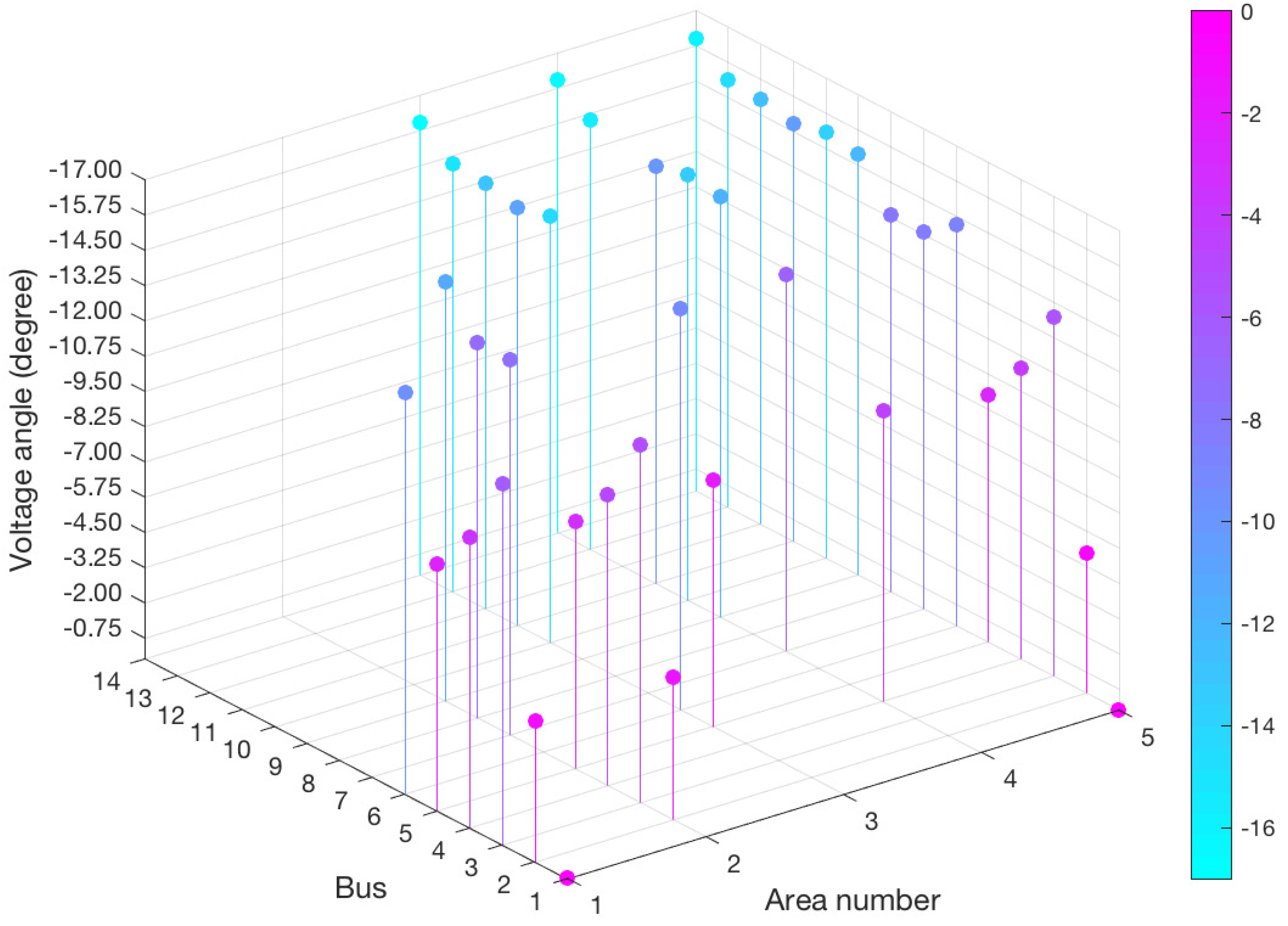
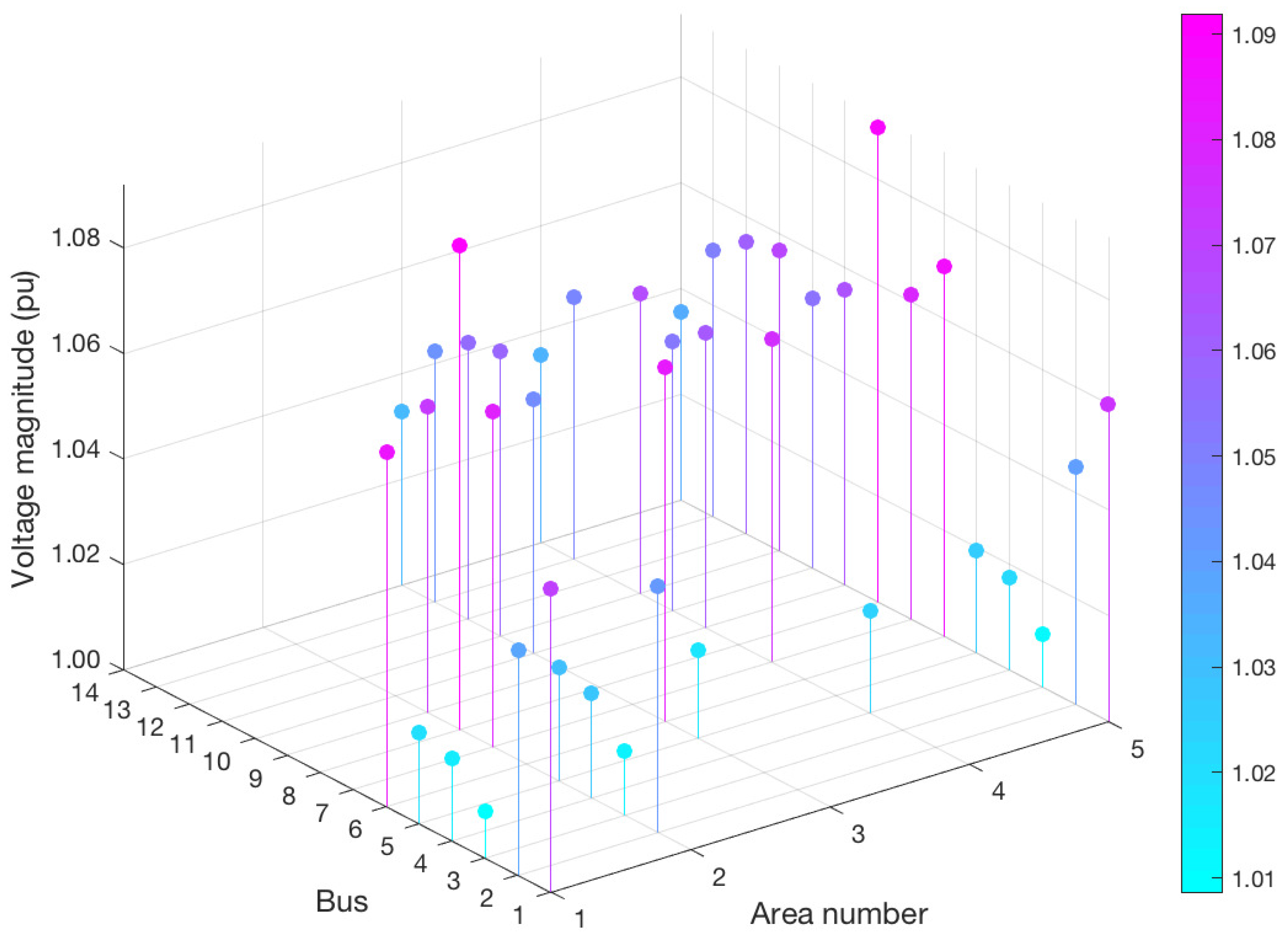
In this case study, the partitioned I E E E -14 bus system is used and illustrated in Figure 1. The multi-area non-linear state estimation model presented previously is applied and, upon convergence, the final estimates of the states are shown in Figure 2 and Figure 3. As shown, in the “Area Number” axis, area number 5 is the power flow solution while the different bars associated with a bus across areas indicate the specific bus is shared with the corresponding areas. The results show that the converged solution are much close to the power flow solution.
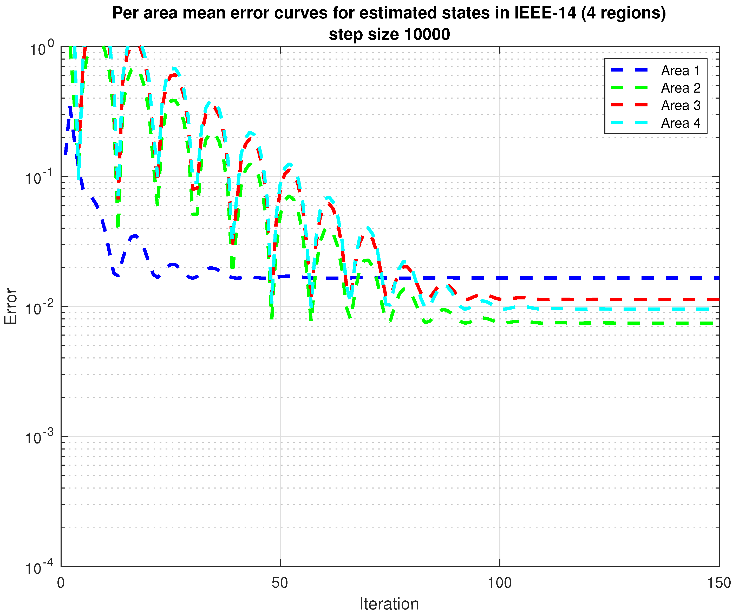
To show the performance of the presented model, the error metric e k = x k x p f 2 / N k in log scale is utilized. A 100 Monte Carlo simulation is generated and the average error curves for each area is shown in Figure 4. From the results, one can see that the presented model is able to achieve a per area mean error smaller than 10−2 within a few more iterations compared to the centralized solution, which in this case took 11 iterations. Using the Monte Carlo simulation, Table 1 and Table 2 present the error statistics per area per state. In other words, the difference between estimated states and power flow solution is calculated for each state. In Table 1, local and shared states are included in the calculation while in Table 2 only local states are considered. Table 2 further presents final estimates of the states in each area.
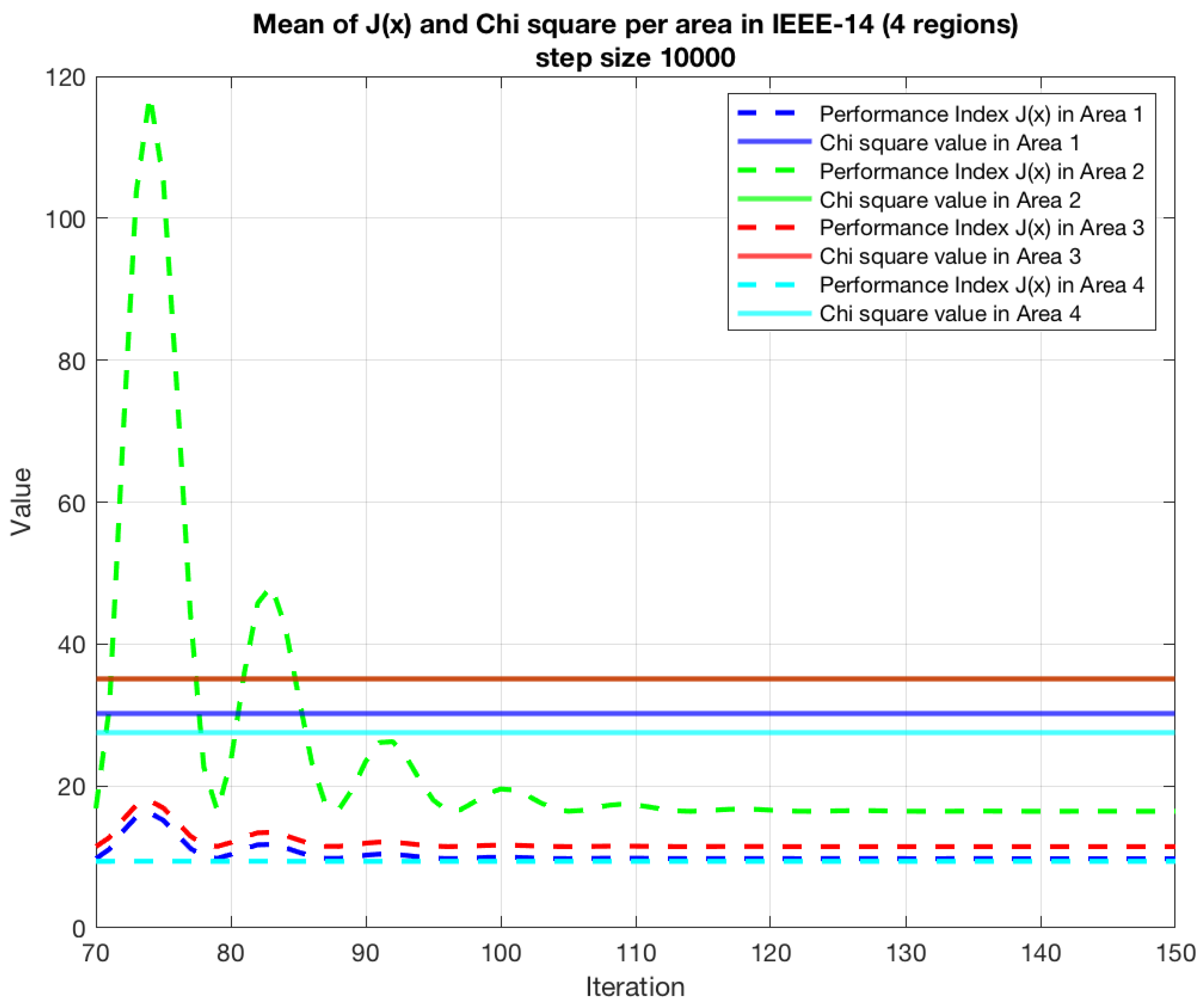
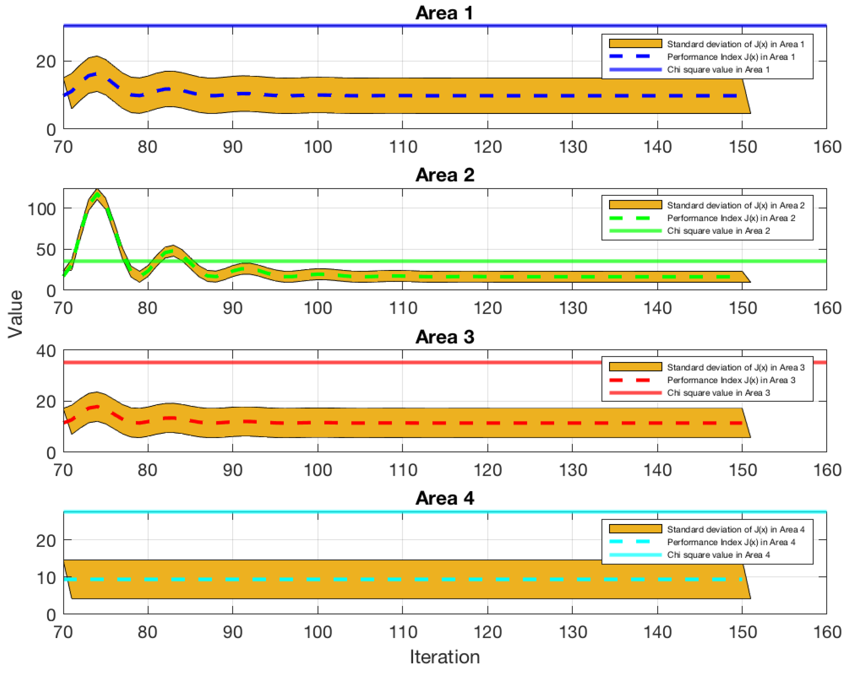
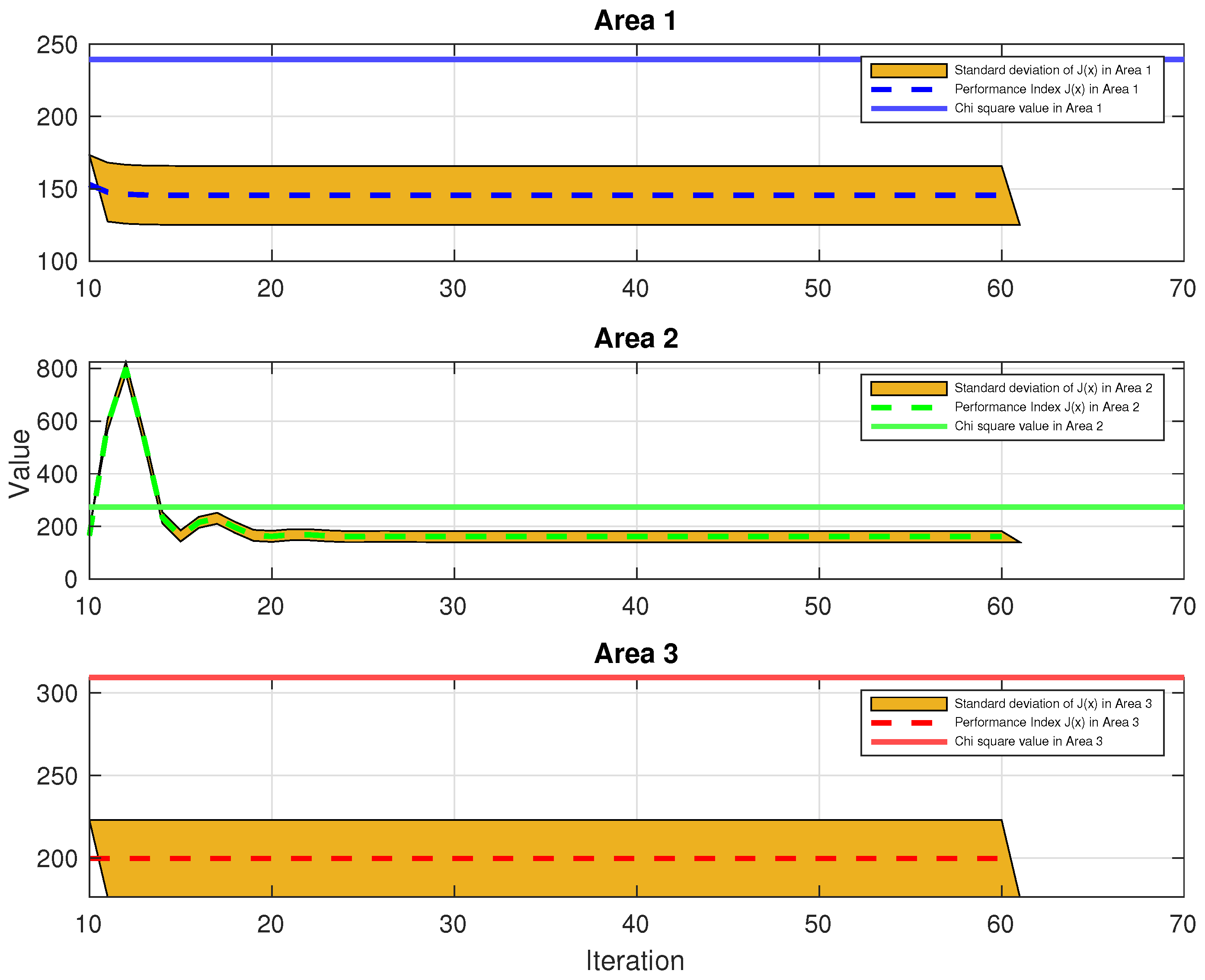
To evaluate the presented model’s robustness, measurements’ noise conditions are simulated. Figure 5 and Figure 6 show the performance index J ( x ) , which is the norm of the measurements error in each area after convergence, over iterations. In this figure, the index J ( x ) and the χ 2 threshold associated with each area are plotted on the same window. As one can see, upon convergence, the performance index is smaller than the threshold value, which indicates that no gross error is present. Hence, the estimated states are optimal and the measurements error are minimal.
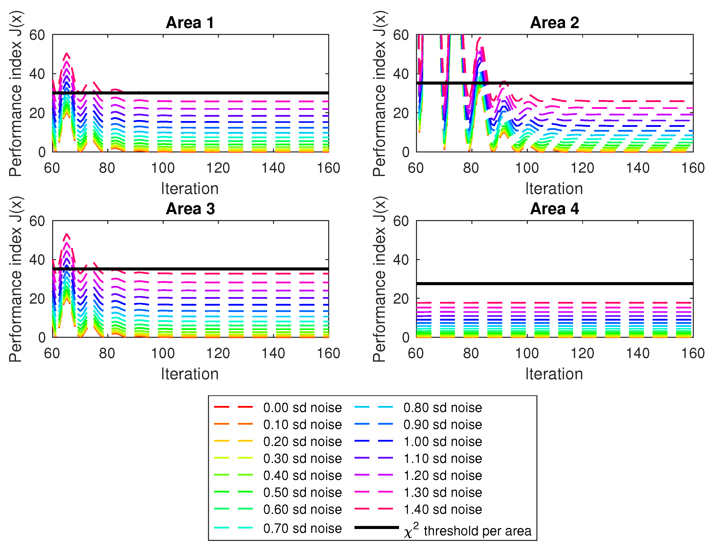
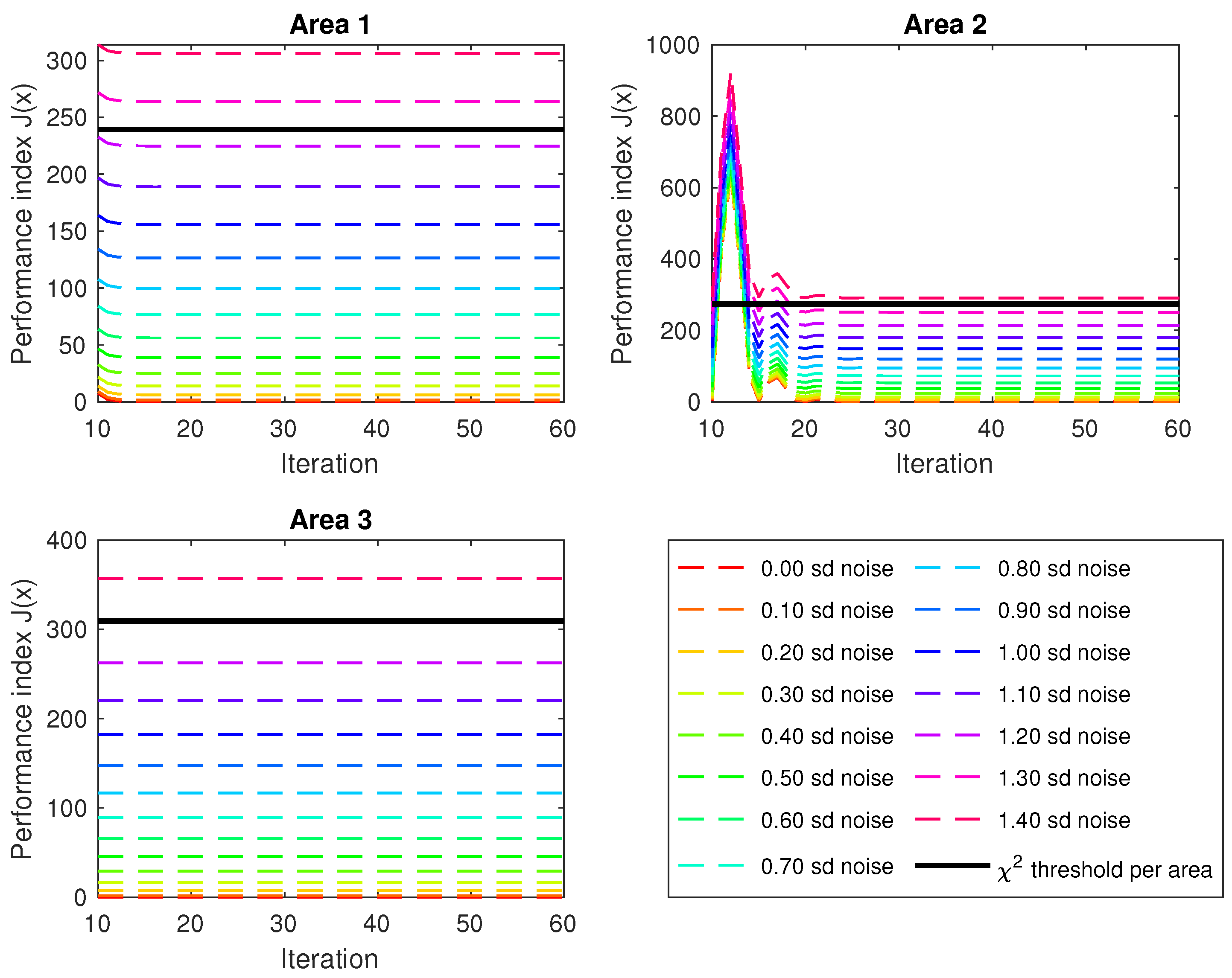
To further analyze the robustness of the presented model, the noise level in the measurements is varied from 0 to 1.4 % of the measurements’ standard deviation (sd). Test result is presented in Figure 7. This figure highlights the effect of noise level in the measurements associated with each area on the performance index J ( x ) . Each area has different χ 2 threshold because of different measurement set across areas. The results show that even with noise level above 1 % , the performance index J ( x ) per area is smaller than the threshold value, which reduces the false positive alarms.

4.2. IEEE-118 Bus System

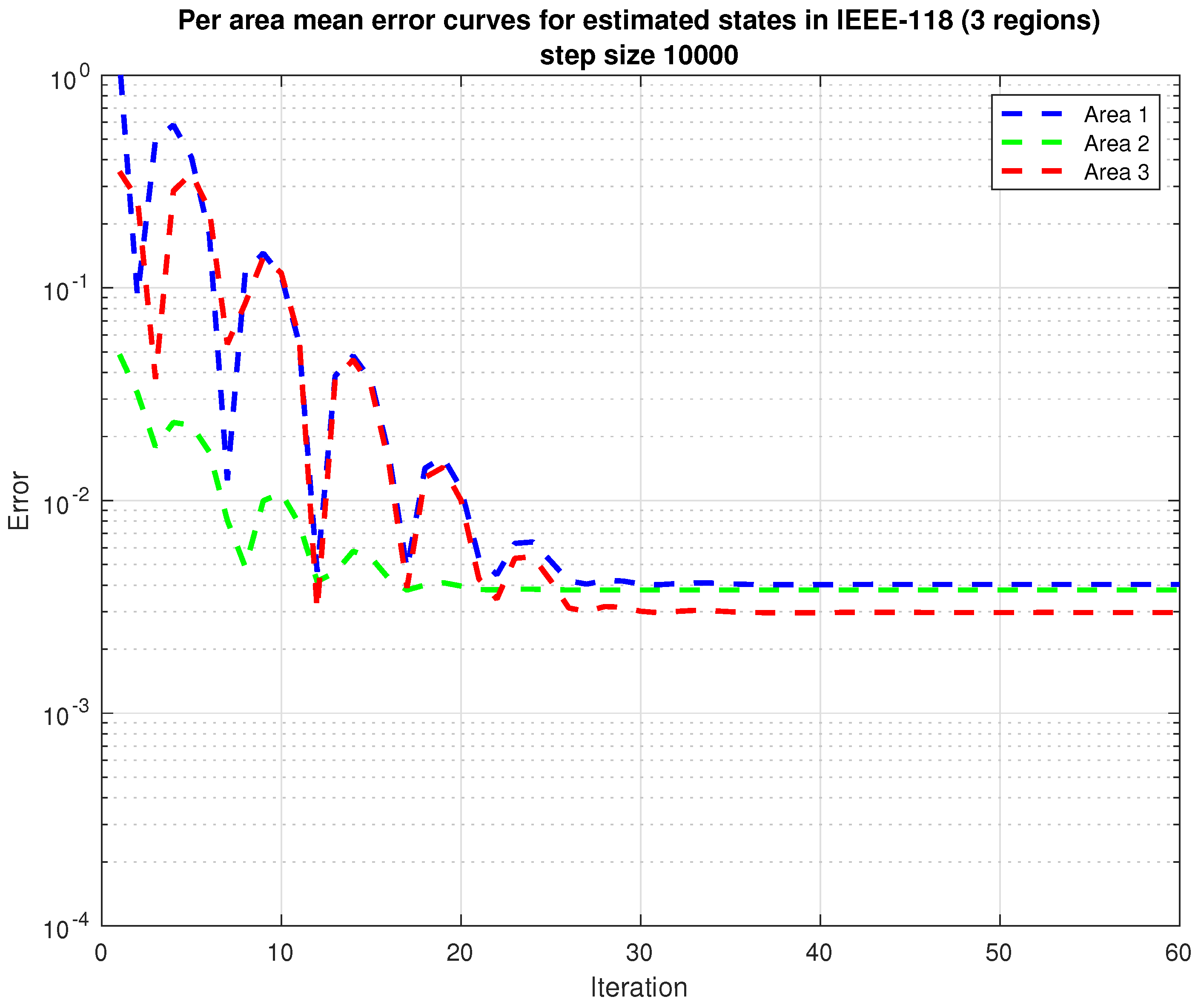
In this case study, the multi-area non-linear state estimation model is applied to a partitioned I E E E -118 bus system. Since the number of states in this system is large compared to the I E E E -14 bus system, it is difficult to visualize the final estimates. However, the same error metric used in the I E E E -14 bus system is applied to this system. Hence, a 100 Monte Carlo simulation is generated and the average error curves for each area is shown in Figure 8. From the shown results, one can see that the presented model has achieved error below the order of 10 2 within less iterations compared to the system in Figure 1. The main reason for such is that the number of shared states within an area is less, which depicts a realistic scenario in real-life. Table 3 and Table 4 present the error statistics per area per state for the considered system. In Table 3, local and shared states are included in the calculation while in Table 4 only local states are considered. Table 4 presents statistics regarding area states final estimates.
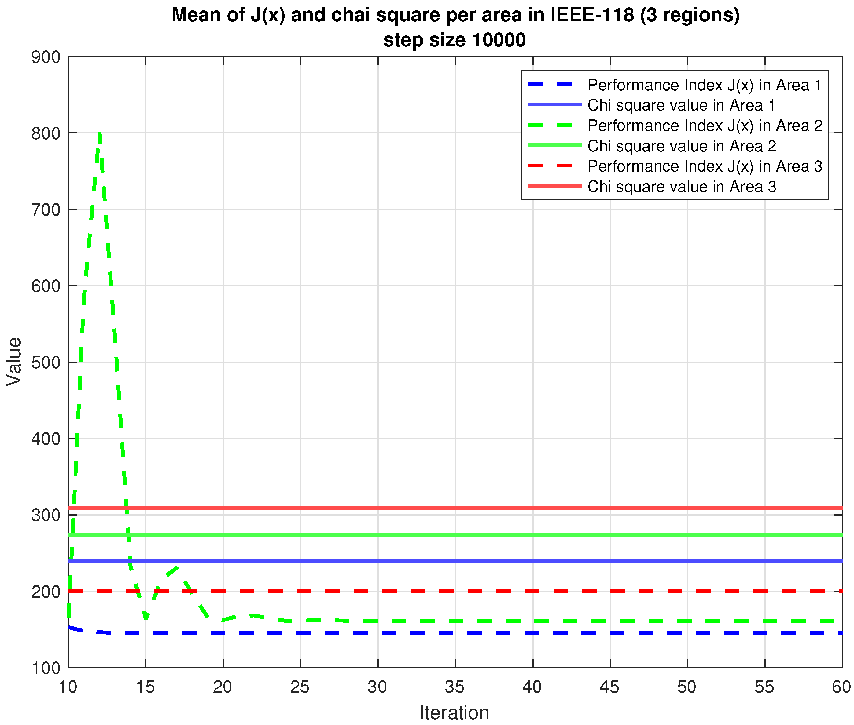
The behavior of the performance index J ( x ) is recorded over the iteration process and is presented in Figure 9 and Figure 10. Upon convergence, the performance index is less than the threshold value. Hence, no gross errors are detected based on χ 2 test.
The robustness the presented model against the noise level in the measurements is also evaluated considering this test system. Similar to the previous case study, the noise level is varied from 0 to 1.4 % of the measurements’ standard deviation. The result is presented in Figure 11. The results show that with noise level up to 1.1 % , the performance index J ( x ) per area is below the threshold value, which reduces the false positive alarms.

5. Conclusions

In this paper, a multi-area nonlinear state estimation model is presented. The model considers the Innovation Index ( I I ) concept, which estimates the masked error component pertaining to the Jacobian null space and then composes the measurement error. The multi-area measurement model is solved with the alternative direction method of multipliers, which enables minimal information sharing. Validation is made considering two I E E E test systems. The two systems are partitioned to emulate different control centers controlling and monitoring interconnected power system. Tests include comparison with the benchmark centralized quasi-static measurement model. Test results statistics regarding robustness to measurement noise and computational speed are analyzed. Presented results show that the model is capable of handling noise in shared states among areas while maintaining computational speed and precision. Further, multi-area model converges to centralized solution within acceptable range of errors. Considering that the majority of utilities companies software rely on a centralized nonlinear state estimation, the presented model can be easily integrated in real-life application without major changes.

Author Contributions

Conceptualization, N.A.; methodology, N.A.; software, N.A. and T.Z.; validation, N.A.; formal analysis, N.A.; investigation, N.A. and T.Z.; resources, N.A.; data curation, N.A.; writing—original draft preparation, N.A.; writing—review and editing, N.A. and T.Z.; visualization, N.A. and T.Z.; supervision, A.S.B. and N.G.B.; project administration, A.S.B.; funding acquisition, A.S.B. All authors have read and agreed to the published version of the manuscript.

Funding

This work was supported by NSF grant ECCS-1809739.

Institutional Review Board Statement

Not applicable.

Informed Consent Statement

Not applicable.

Data Availability Statement

Data is contained within the article or supplementary material.

Conflicts of Interest

The authors declare no conflict of interest.

References

  1. Schweppe, F.C.; Wildes, J. Power system static-state estimation, Part I: Exact model. In IEEE Transactions on Power Apparatus and Systems; IEEE: Piscataway, NJ, USA, 1970; pp. 120–125. [Google Scholar]
  2. Cecati, C.; Mokryani, G.; Piccolo, A.; Siano, P. An overview on the smart grid concept. In Proceedings of the IECON 2010—36th Annual Conference on IEEE Industrial Electronics Society, Glendale, CA, USA, 7–10 November 2010; IEEE: Piscataway, NJ, USA, 2010; pp. 3322–3327. [Google Scholar]
  3. McDaniel, P.; McLaughlin, S. Security and privacy challenges in the smart grid. IEEE Secur. Priv. 2009, 7, 75–77. [Google Scholar] [CrossRef]
  4. Korres, G.N. A distributed multiarea state estimation. IEEE Trans. Power Syst. 2010, 26, 73–84. [Google Scholar] [CrossRef]
  5. Korres, G.N.; Tzavellas, A.; Galinas, E. A distributed implementation of multi-area power system state estimation on a cluster of computers. Electr. Power Syst. Res. 2013, 102, 20–32. [Google Scholar] [CrossRef]
  6. Jiang, W.; Vittal, V.; Heydt, G.T. A distributed state estimator utilizing synchronized phasor measurements. IEEE Trans. Power Syst. 2007, 22, 563–571. [Google Scholar] [CrossRef]
  7. Gomez-Exposito, A.; Abur, A.; de la Villa Jaen, A.; Gomez-Quiles, C. A multilevel state estimation paradigm for smart grids. Proc. IEEE 2011, 99, 952–976. [Google Scholar] [CrossRef]
  8. Jiang, W.; Vittal, V.; Heydt, G.T. Diakoptic state estimation using phasor measurement units. IEEE Trans. Power Syst. 2008, 23, 1580–1589. [Google Scholar] [CrossRef]
  9. Zhao, L.; Abur, A. Multi area state estimation using synchronized phasor measurements. IEEE Trans. Power Syst. 2005, 20, 611–617. [Google Scholar] [CrossRef]
  10. Ebrahimian, R.; Baldick, R. State estimation distributed processing [for power systems]. IEEE Trans. Power Syst. 2000, 15, 1240–1246. [Google Scholar] [CrossRef]
  11. Zhu, H.; Giannakis, G.B. Power system nonlinear state estimation using distributed semidefinite programming. IEEE J. Sel. Top. Signal Process. 2014, 8, 1039–1050. [Google Scholar] [CrossRef]
  12. Xie, L.; Choi, D.H.; Kar, S.; Poor, H.V. Fully distributed state estimation for wide-area monitoring systems. IEEE Trans. Smart Grid 2012, 3, 1154–1169. [Google Scholar] [CrossRef]
  13. Min, L.; Abur, A. Total transfer computation for multi-area power systems. IEEE Trans. Power Syst. 2006, 21, 1141–1147. [Google Scholar] [CrossRef]
  14. Conejo, A.J.; de la Torre, S.; Canas, M. An optimization approach to multiarea state estimation. IEEE Trans. Power Syst. 2007, 22, 213–221. [Google Scholar] [CrossRef]
  15. Kekatos, V.; Giannakis, G.B. Distributed robust power system state estimation. IEEE Trans. Power Syst. 2012, 28, 1617–1626. [Google Scholar] [CrossRef] [Green Version]
  16. Monticelli, A. State Estimation in Electric Power Systems: A Generalized Approach; Springer Science & Business Media: Berlin, Germany, 1999; Volume 507. [Google Scholar]
  17. Abur, A.; Expósito, A. Power System State Estimation: Theory and Implementation; Power Engineering (Willis), CRC Press: Boca Raton, FL, USA, 2004. [Google Scholar]
  18. Gómez-Expósito, A.; de la Villa Jaén, A.; Gómez-Quiles, C.; Rousseaux, P.; Van Cutsem, T. A taxonomy of multi-area state estimation methods. Electr. Power Syst. Res. 2011, 81, 1060–1069. [Google Scholar] [CrossRef] [Green Version]
  19. Bretas, N.G.; Bretas, A.S. A two steps procedure in state estimation gross error detection, identification, and correction. Int. J. Electr. Power Energy Syst. 2015, 73, 484–490. [Google Scholar] [CrossRef]
  20. Bretas, N.G.; Bretas, A.S. The Extension of the Gauss Approach for the Solution of an Overdetermined Set of Algebraic Non Linear Equations. IEEE Trans. Circ. Syst. II Express Briefs 2018, 65, 1269–1273. [Google Scholar] [CrossRef]
  21. Boyd, S.; Parikh, N.; Chu, E. Distributed Optimization and Statistical Learning via the Alternating Direction Method of Multipliers; Now Publishers Inc.: Delft, The Netherlands, 2011. [Google Scholar]
  22. Zimmerman, R.D.; Murillo-Sánchez, C.E.; Thomas, R.J. MATPOWER: Steady-state operations, planning, and analysis tools for power systems research and education. IEEE Trans. Power Syst. 2010, 26, 12–19. [Google Scholar] [CrossRef] [Green Version]
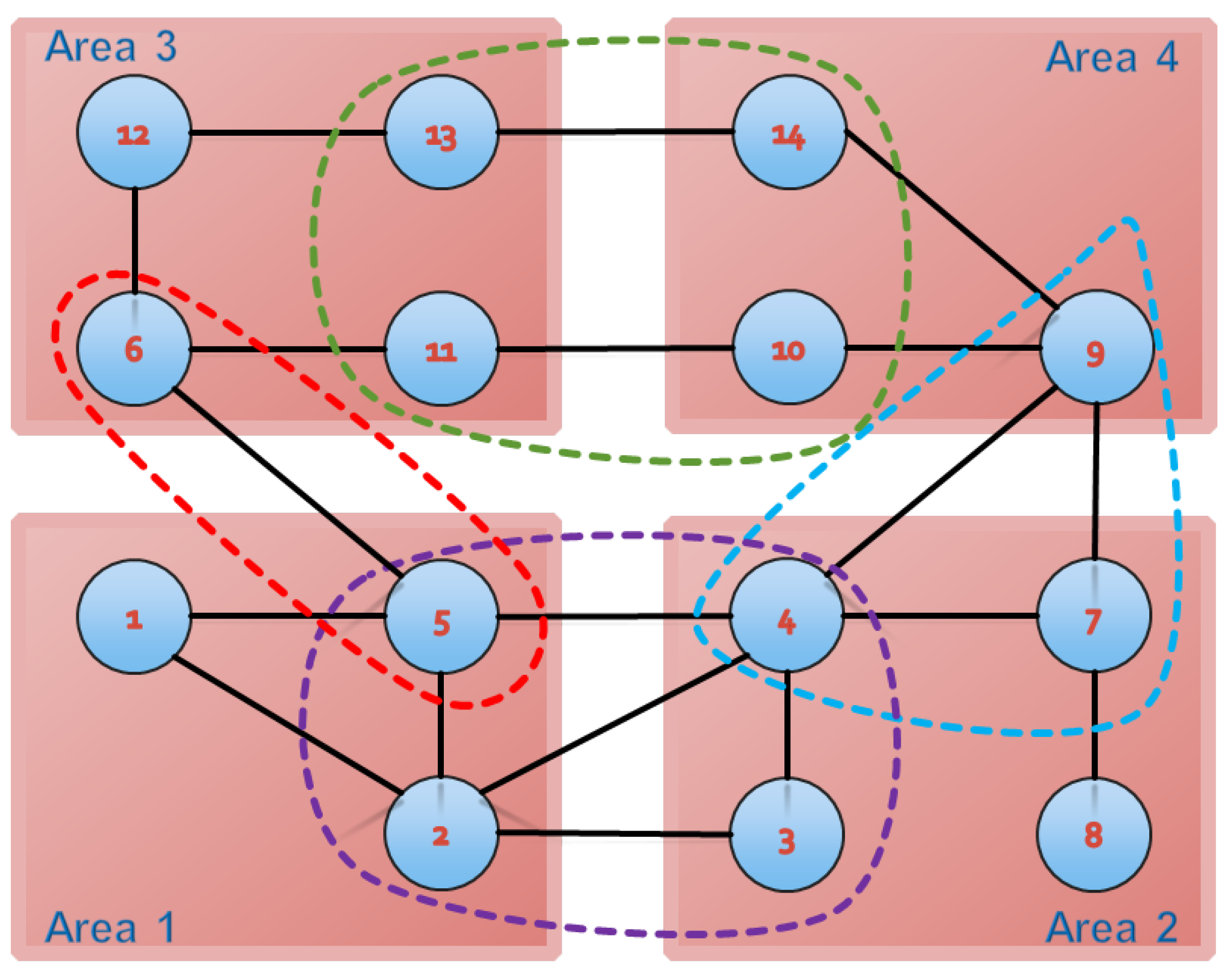
Figure 1. I E E E -14 bus system divided into four areas. Dotted lassos shows the the boundary buses between areas.
Applsci 11 04419 g001
Figure 2. Estimated state (angles) on the I E E E -14 bus system 4 regions.
Applsci 11 04419 g002
Figure 3. Estimated state (magnitude) on the I E E E -14 bus system 4 regions.
Applsci 11 04419 g003
Figure 4. Per area error curves on the I E E E -14 bus system 4 regions.
Applsci 11 04419 g004
Figure 5. Per area mean of J(x) on the I E E E -14 bus system 4 regions.
Applsci 11 04419 g005
Figure 6. Per area mean of J(x) on the I E E E -14 bus system 4 regions with standard deviation.
Applsci 11 04419 g006
Figure 7. Performance index for different noise level on the I E E E -14 bus system 4 regions.
Applsci 11 04419 g007
Figure 8. Per area error curves on the I E E E -118 bus system 3 regions.
Applsci 11 04419 g008
Figure 9. Per area mean of J(x) on the IEEE-118 bus system 3 regions.
Applsci 11 04419 g009
Figure 10. Per area mean of J(x) on the IEEE-118 bus system 3 regions with standard deviation.
Applsci 11 04419 g010
Figure 11. Performance index for different noise level on the IEEE-118 bus system 3 regions.
Applsci 11 04419 g011
Table 1. Statistic metric per state per area on I E E E -14.
StateArea 1Area 2Area 3Area 4
MeanAngle (degree) 1.43 e 2 2.40 e 2 2.19 e 2 2.36 e 2
Magnitude (pu) 0.8 e 3 1.7 e 3 1.4 e 3 1.5 e 3
Average std.Angle (degree) 1.09 e 2 1.79 e 2 1.69 e 2 1.81 e 2
Magnitude (pu) 0.6 e 3 1.2 e 3 0.9 e 3 1.0 e 3
Table 2. Statistic metric per state per area on I E E E -14 (local states only).
StateArea 1Area 2Area 3Area 4
MeanAngle (degree) 0.25 e 2 1.29 e 2 1.21 e 2 1.02 e 2
Magnitude (pu) 0.49 e 3 0.98 e 3 0.80 e 3 0.63 e 3
Average std.Angle (degree) 0.21 e 2 0.97 e 2 0.96 e 2 0.81 e 2
Magnitude (pu) 0.35 e 3 0.69 e 3 0.53 e 3 44 e 3
Table 3. Statistic metric per state per area on I E E E -118.
StateArea 1Area 2Area 3
MeanAngle (degree) 1.17 e 2 1.26 e 2 1.35 e 2
Magnitude (pu) 0.39 e 3 0.35 e 3 0.31 e 3
Average stdAngle (degree) 0.85 e 2 0.91 e 2 1.07 e 2
Magnitude (pu) 0.33 e 3 0.30 e 3 0.22 e 3
Table 4. Statistic metric per state per area on I E E E -118 (local states only).
StateArea 1Area 2Area 3
MeanAngle (degree) 1.01 e 2 0.79 e 2 1.27 e 2
Magnitude (pu) 0.35 e 3 0.29 e 3 0.30 e 3
Average std.Angle (degree) 0.74 e 2 0.58 e 2 1.0 e 2
Magnitude (pu) 0.29 e 3 0.25 e 3 0.21 e 3
Publisher’s Note: MDPI stays neutral with regard to jurisdictional claims in published maps and institutional affiliations.