Article

Comparison of the Shear Modulus of an Offshore Elastomeric Bearing between Numerical Simulation and Experiment

1
Department of Mechanical Engineering, Dong-A University, Busan 49315, Korea
2
Department of Mechatronics Engineering, Kyungsung University, Busan 48434, Korea
*
Author to whom correspondence should be addressed.
Appl. Sci. 2021, 11(10), 4384; https://doi.org/10.3390/app11104384
Submission received: 5 April 2021 / Revised: 10 May 2021 / Accepted: 10 May 2021 / Published: 12 May 2021
(This article belongs to the Section Mechanical Engineering)

Abstract

:
The most important item when indicating the mechanical properties of offshore elastomeric bearings is the shear modulus, and the method of measuring this is shown in EN 1337-3, a regulation related to offshore elastomeric bearings. In this work, we conducted an experimental and numerical study on an offshore elastomeric bearing to find its shear modulus. Shear modulus tests were conducted according to the procedure specified in EN 1337-3 Annex F, while simulations were performed using the finite element analysis (FEA) software, ANSYS. The main objective of this research work is to determine optimum analysis conditions for the simulation method that considers a nonlinear model for the elastomer material and predicts the experimental results accurately. We considered the Mooney–Rivlin (M-R) model that has two-parameter (2P), five-parameter (5P), and nine-parameter (9P) forms, depending on the number of terms in the series. We observed that the load-displacement graph is linear, and the percentage error between the results obtained with 2P and 5P M-R models is around 2.23% in the compression and 0.38% in the shear. The simulation results from 2P M-R model showed a good agreement with the experimental results with the correlation coefficient (R2) being 0.999 with an average error of about 2%. However, the deviation between the experimental and simulation results from the 9P M-R model is very high, with about 7%. Based on this study, we can say that the 2P M-R model can accurately predict the nonlinear behavior of hyperelastic material used in elastomer bearing. In addition, the shear modulus of elastic bearings for Class 3 Shore hardness was verified by comparing the numerical simulation values with those presented in EN 1337-3 Annex D.

1. Introduction

Elastomeric bearings for FPSO are located at the interfaces between topside modules and support stools on the deck of the offshore platform. Their major function is to minimize the structural interactions of the two bodies. Particularly, they shall reduce the shear loads and bending moments in the module plate girders supported on the stools. These bearings are manufactured by intersecting an elastomer made of neoprene and reinforcing steel plates in the same way as for land use [1,2]. Land elastomeric bearings are used in bridges and buildings so that they support high-frequency repetitive loads caused by earthquakes [3,4,5]. Unlike those land elastomeric bearings subjected to repeated loads, the offshore elastomeric bearings are to firmly support the heavy upper module from the wind load and motion of hull in various sea environments including towing, operating, and extreme conditions [6,7,8]. So, an offshore elastomeric bearing is larger in size and stronger in rigidity than that for land use, and it tends to have a square block shape to effectively support the translational and rotational movements of upper topside modules caused by 6DOF (degree of freedom) hull motions (surge, sway, heave, roll, pitch, yaw) [9]. In addition, since loads vary with types of modules on the platform, offshore elastomer bearings should have adequate shear stiffness to minimize their horizontal movements while elastically supporting the vertical loads [10].
The most important item when indicating the mechanical properties of such offshore elastomeric bearings is the shear modulus, and the method of measuring this is shown in EN 1337-3 [11], a regulation related to offshore elastomeric bearings. In the previous study [12] that analyzed the effect of reinforcing plate on the stiffness of elastomer bearing, the influence of reinforcing plate was dominant on compressive stiffness and bending stiffness. It was confirmed that the height ratio to the cross-sectional area mainly is affected. In addition, according to the EN 1337-3 regulation, it can be seen that the shore hardness of the elastomer is closely related to the shear modulus of the bearing. Many experimental and numerical studies have been reported on the effect of various parameters on the mechanical behavior of elastomeric bearings [13,14,15,16,17]. Konstantinidis et al. [13] performed an experimental analysis on the seismic response of three types of steel-reinforced elastomeric bearings (SREBs) used in bridges. They concluded that all SREBs they analyzed performed exceptionally well under seismic loading. Steelman et al. [14] conducted experiments on SREBs attached to a concrete layer on one side and bounded on the other side. They observed that shear strain increases nonlinearly with vertical load (compressive pressure). Li and Wu [15] experimentally studied the ultimate state of shear failure and the friction sliding performance of SREBs in bridges. Peng et al. [16] performed experimental tests on natural rubber-laminated bearings for bridges to investigate the effects of vertical load and peak acceleration of ground motion. They also performed numerical simulations using a finite element method and proposed an accurate method for calculating seismic responses of bridges with laminated bearings. Recently, Kaloo et al. [17] investigated the effect of various parameters on the mechanical properties of SREBs under large shear deformations numerically and experimentally. In all the literature mentioned above, experimental and/or numerical studies were conducted on elastomeric bridge-bearings only. However, till now, there have been no studies on finding the shear modulus of an offshore elastic bearing by using the EN 1337-3 regulation procedure to the authors’ knowledge. The reason is that the size of marine elastomer bearings is significantly larger than that for land use, and the applied load reaches thousands of tons, so experiments cannot be carried out with existing equipment. In addition, the method and regulations for measuring the shear modulus of elastomeric bearings for land and offshore are different, so the results of existing studies on bridge bearings cannot be applied to offshore applications. Therefore, the necessity of this research work is to analyze the shear modulus of offshore elastomeric bearings according to the procedure mentioned in EN 1337-3 regulation.
Offshore elastomeric bearings must be physically tested with full-size products in accordance with EN 1337-3 regulation. However, the experimental set-up incurs high cost due to large capacity of the test equipment and a dedicated shear test device. On the other hand, the numerical simulation can analyze various conditions at low cost, but in order to accurately analyze elastomers, which are hyperelastic (nonlinear) materials, it is necessary to find suitable analysis conditions. Therefore, finding the optimum analysis conditions for the numerical simulation technique that reproduce corresponding experimental results is necessary. The most crucial step in predicting the nonlinear behavior of a hyperelastic material through numerical simulations is considering the correct nonlinear model. When performing numerical simulations for hyperelastic materials such as rubber, the first-order, two-parameter (2P) Mooney–Rivlin (M-R) model is mainly used, which has a good response in compression within 30% and tension within 200%. On the contrary, the error is substantial in tensions of 200% or more. In this case, the responsiveness can be improved by using the 5P and 9P M-R models for the material behavior [18,19,20]. In this study, three types of M-R models, such as 2P (first-order), 5P (second-order), and 9P (third-order), are used to increase the reliability of numerical simulation for offshore elastomeric bearings. The main objective of this research work is to propose a suitable M-R model for simulating the behavior of an elastomeric bearing under compression and shear tests by comparing and analyzing load-displacement graphs obtained with 2P, 5P, and 9P models with the experiment. Overall aim is to match the simulation results of elastomeric bearing’s shear modulus values with the experimental results. The research procedure for this is as follows: First, actual-sized offshore elastomeric bearing specimens are fabricated, and the experiment was conducted according to the procedure specified in EN 1337-3 Annex F: Shear Modulus Test. Second, the numerical simulation of the elastomeric bearing with respect to the behavior model of hyperelastic material was performed for the same conditions as the experiment. Third, after obtaining a shear force-displacement graph in both the experiment and the numerical simulation, the shear modulus is calculated and compared by using the slope of the graph. Last, the shear modulus of the elastomeric bearing with respect to the shore hardness was verified by comparing the numerical simulation values with the values presented in EN 1337-3 Annex D. A 2500-ton press equipped with a shear test device with a capacity of 300-tons is used for the experiment, and ANSYS Mechanical APDL [21], a general-purpose finite element analysis program, is used for numerical simulation.

2. Experimental Procedure and Findings

2.1. Materials and Methods

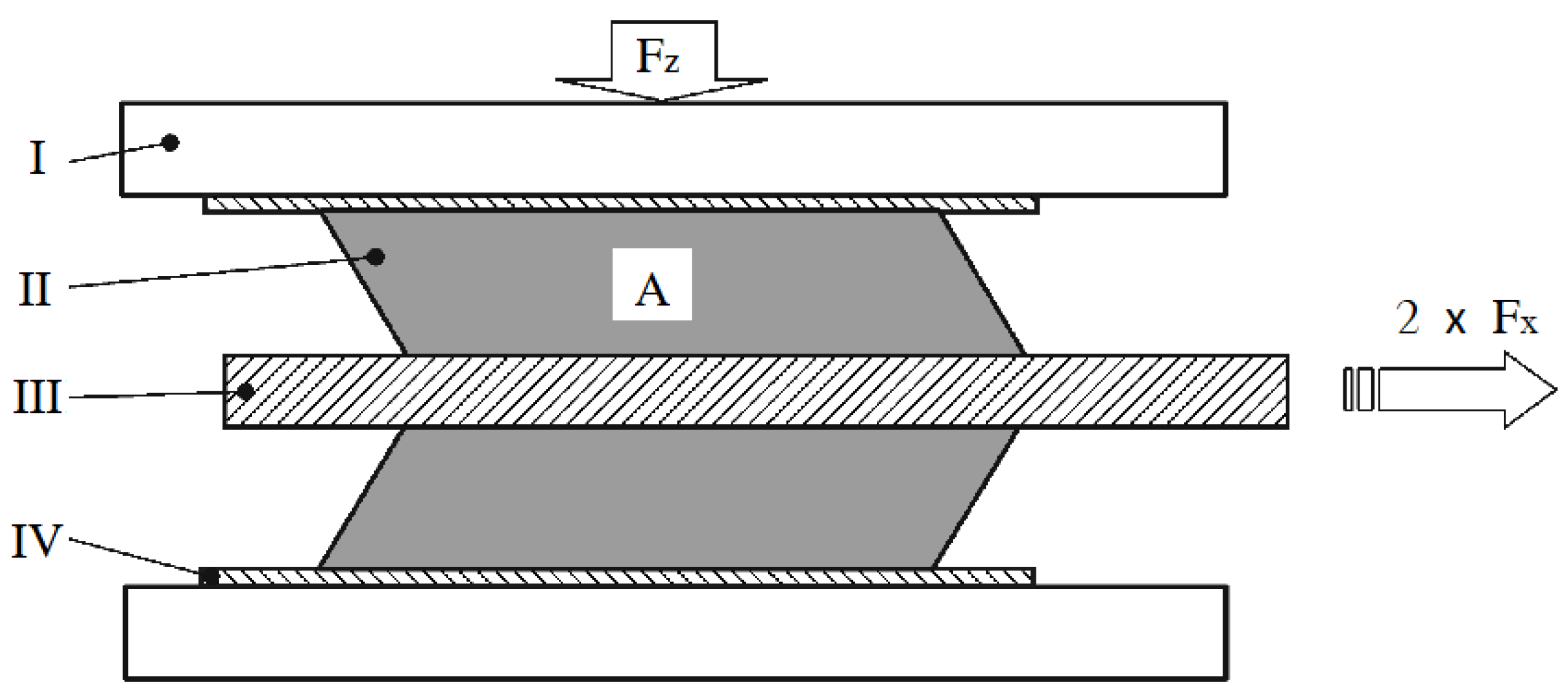
The shear modulus test procedure according to EN 1337-3 Annex F is as follows: The test pieces shall be placed symmetrically on each side of the movable plate so that the shear direction is across the width of the bearing. A mean pressure of 6 MPa shall be applied. The bearings shall be subjected to shear at a constant and maximum speed of 150 mm/minute to the maximum test deflection Dxm (0.7 Tq ≤ Dxm ≤ 0.9 Tq) and then returned to zero deflection. The compressive stress shall be removed and the test pieces left undisturbed for five minutes and then sheared again to Dxm. The horizontal deflection and force shall be recorded continuously or at a minimum of 10 equal intervals during the loading part of the cycle. The experimental conditions for the shear modulus test is shown in Figure 1.
According to EN 1337-3 Annex F, the conventional shear modulus Gg, in MPa, is obtained from the measurements, using an equation:
G g = ( τ s 2 τ s 1 ) ( ε q x 2 ε q x 1 )
where, τs2 is the shear stress and εqx2 the shear strain at a deformation Dx2 = 0.58 × Tq = 75.4 mm, τs1 is the shear stress and εqx1 the shear strain at a deformation Dx1 = 0.27 × Tq = 35.1 mm, Tq is the thickness of elastomer (in this specimen Tq = 130 mm), τs is the shear stress: τs = Fx/A (in this specimen A = L × B = 800 × 800 = 640,000 mm2), Fx is the horizontal force (shear force) and εqx is the shear strain: εqx = Dx/Tq.

2.2. Test Model and Instrument

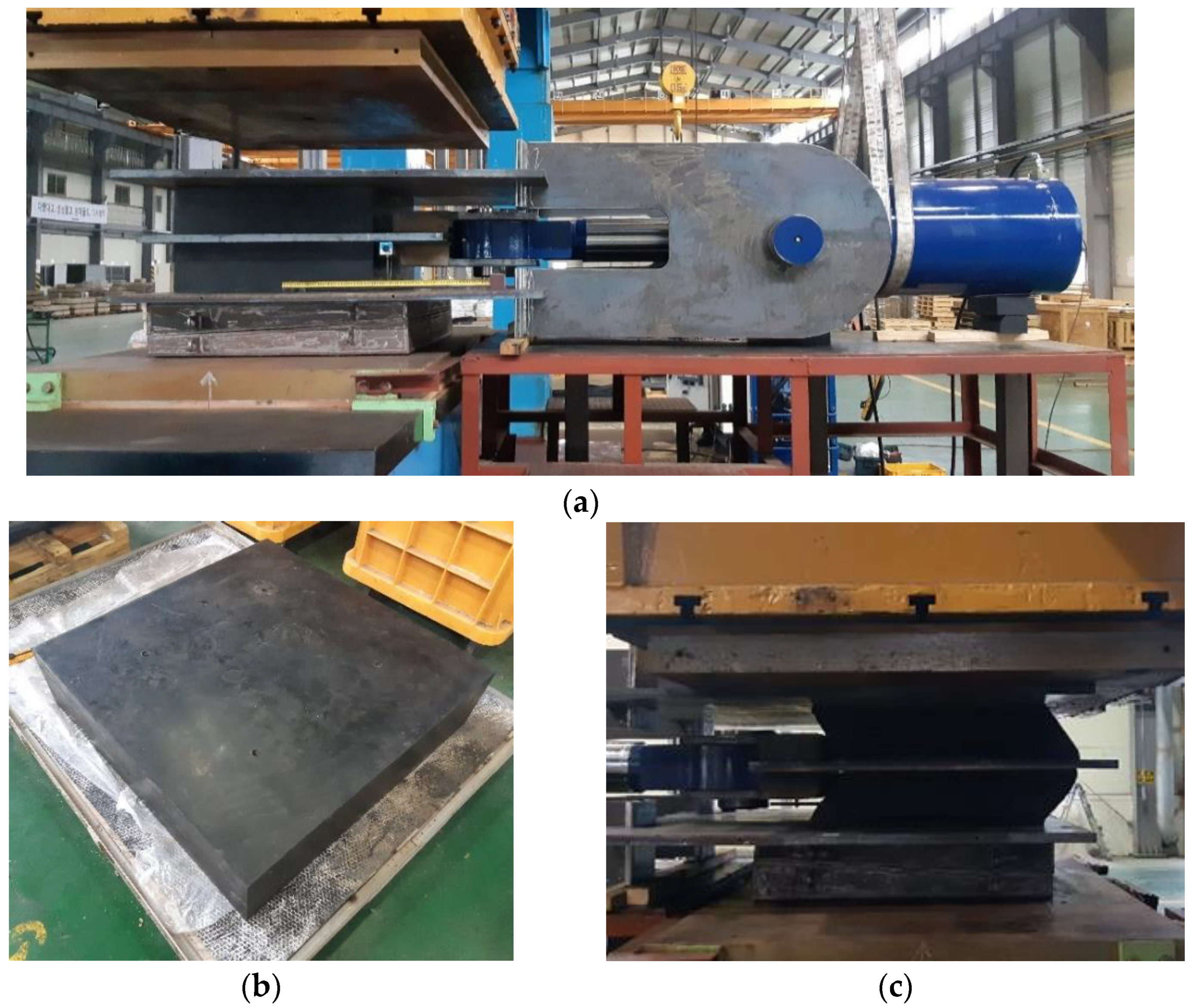
Offshore elastomer bearings are divided into a vertical bearing that supports the upper module and a horizontal bearing that blocks side movement. Since the vertical bearing is the main part, this study deals with the vertical bearing only. Vertical elastomeric bearings generally have a size of 600 × 600 mm~1400 × 1400 mm, and in order to measure the shear modulus, a bearing with an area of 800 × 800 mm suitable for the capacity of the test device is selected as a test model. The height of the test specimen is 200 mm, and three reinforcing plates of 6 mm thickness are inserted into the elastomer in the middle of two contact plates of 25 mm thickness at the top and bottom. Two test specimens of the same size are fabricated in accordance with EN 1337-3: Annex F, which is the shear modulus test standard. The compression/shear test instrument, test specimen, and shear test condition are shown in Figure 2.

2.3. Experimental Results

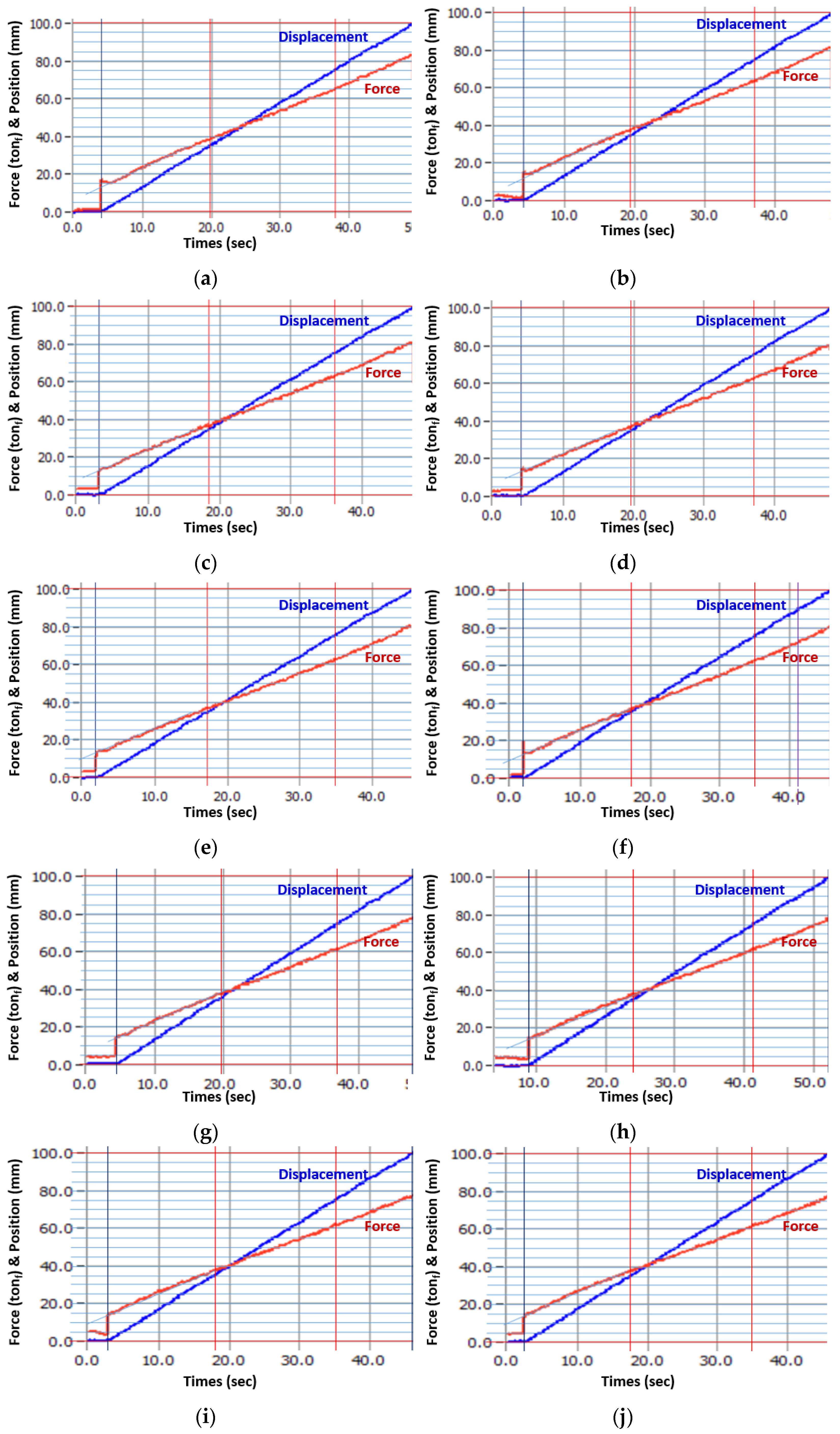
The shear modulus test conditions according to EN 1337-3 and actual test values are shown in Table 1. The shear force and displacement graphs measured through the performance evaluation (average values of 10 tests under the same conditions) are shown in Figure 3.
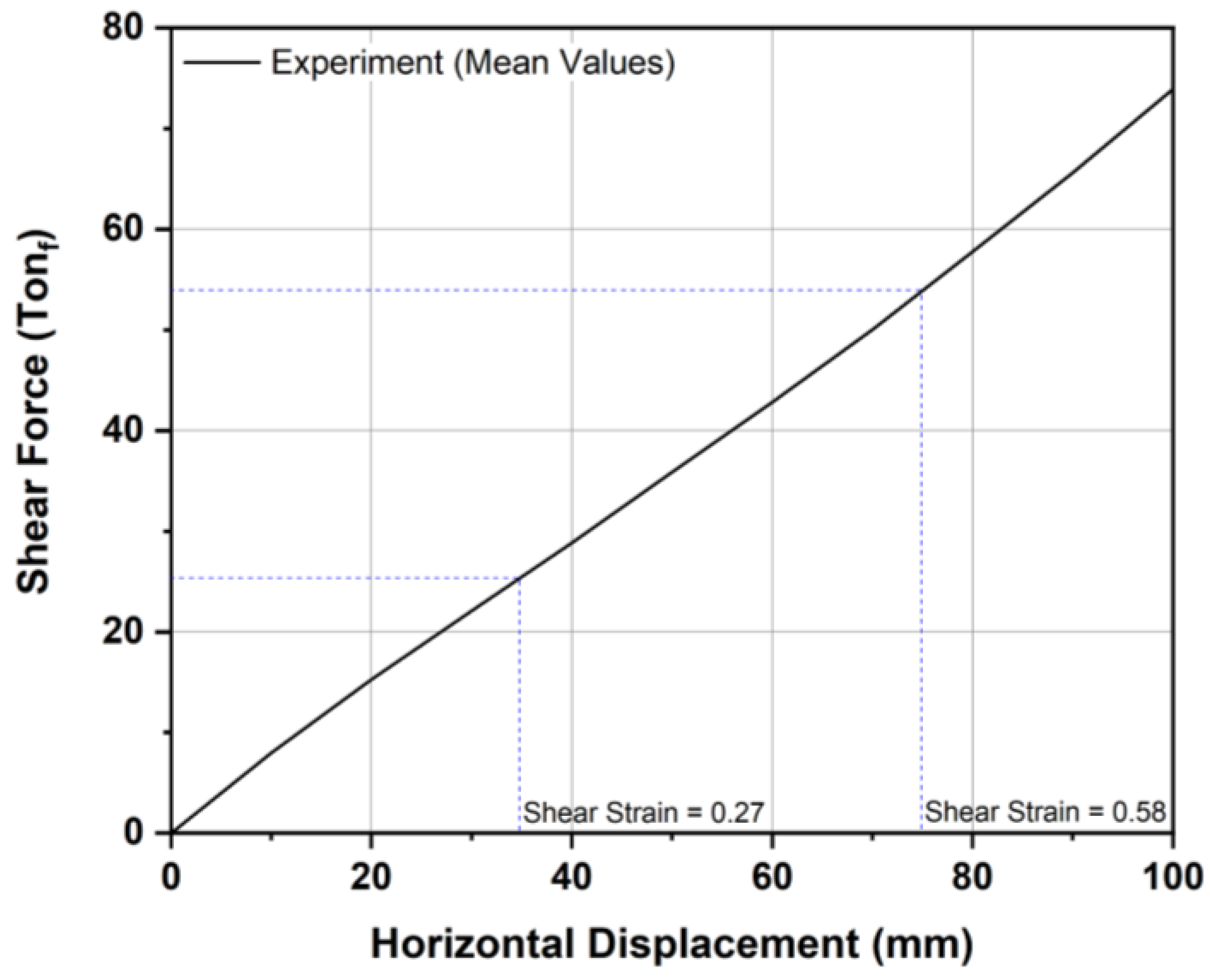
In order to calculate the shear modulus of the elastomeric bearing specimen, the mean values of 10 tests are plotted in Figure 4 as the shear force–displacement graph. In Figure 4, the mean forces at two strain points (0.27 and 0.58) are found, and the factors required for calculating the shear modulus are shown in Table 2. Since the shear test was performed by stacking two bearings, the shear force (Fx) acting on each bearing is calculated by dividing the measured force by 2.
Substituting the values in Table 2 into Equation (1), the conventional shear modulus Gg of the test specimen is calculated as below:
G g = ( τ s 2 τ s 1 ) ( ε q x 2 ε q x 1 ) = ( 0.413 0.195 ) ( 0.58 0.57 ) = 0.707   MPa
As a result of the test, the shear modulus of the specimen is found to be 0.707 MPa, and according to Table 3, which shows EN 1337-3 Annex D: Shear Modulus Comments, it can be seen that this value corresponds to shore A hardness 50 + 5 grade.

3. Numerical Simulation and Results

3.1. Analysis Model

In the numerical simulation of elastomeric bearings, it is very important to consider a proper M-R model for finding the nonlinear behavior of materials accurately. In the case of hyperelastic materials such as rubber, the Mooney–Rivlin (M-R) model is generally used, and, depending on the number of terms in the series, there are mainly three kinds of M-R models, such as 2P (first-order), 5P (second-order), and 9P (third-order). In order to find the most suitable model for numerical simulation of elastomeric bearings, the finite element analysis (FEA) for the compression and shear tests were performed with the above three types of M-R models and compared with experimental results. Numerical simulations were performed on the same domain size (800 × 800 × 200 mm) as the experimental specimen.
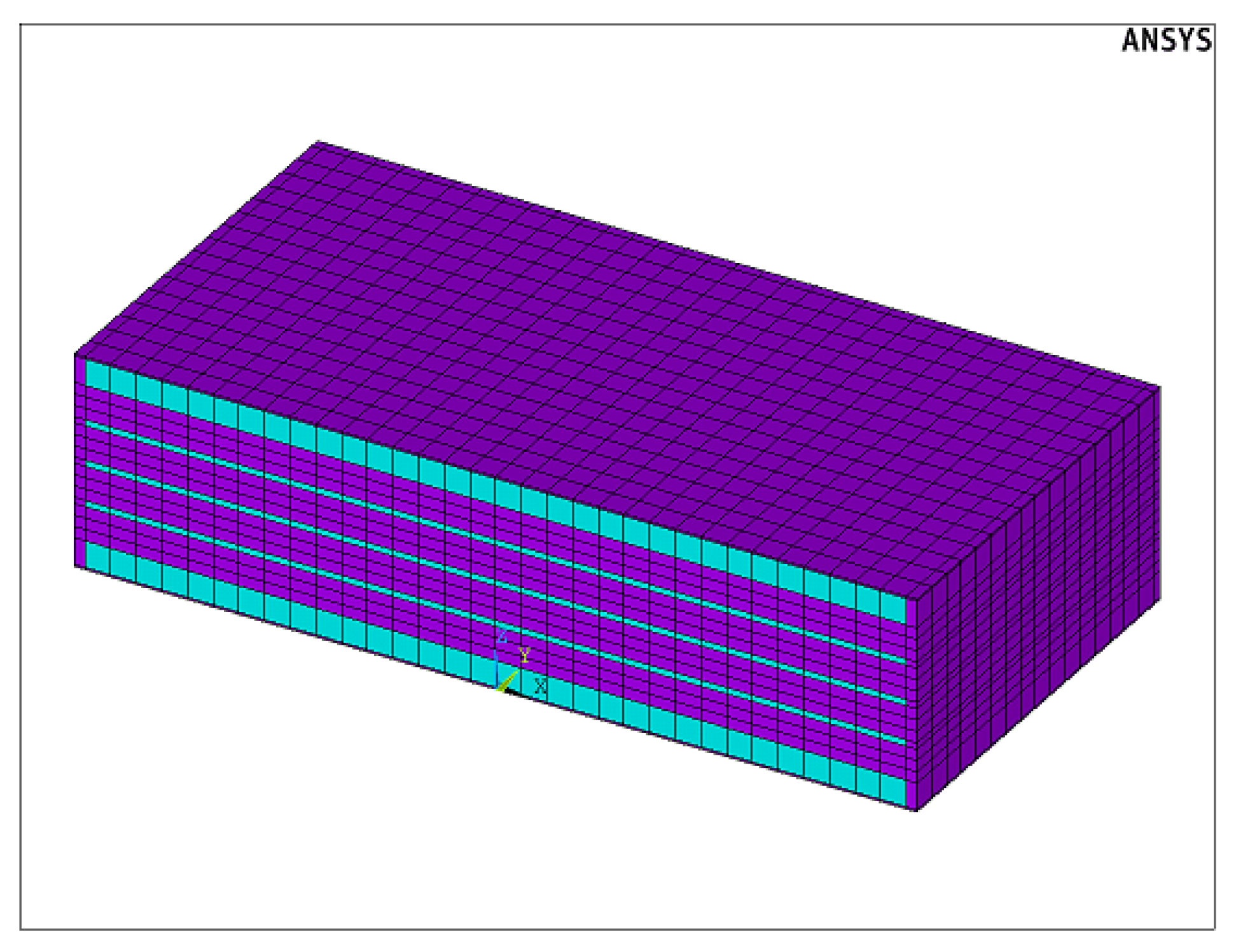
The finite element model for structural analysis of the elastomeric bearing was created so that the length of one side did not exceed 25 mm using an 8-node brick element with 3 degrees of freedom. The number of elements along the thickness direction of the elastomer layer between the reinforcing plates should be set to three or more because elastomer is a nonlinear material. Since the thickness of the elastomer layer is 32 mm, a finite element model was created by dividing the elastomer layer between the reinforcing plates into three, so that the aspect ratio of the brick element is 0.4 or more. Only half of the domain was modeled as the geometric shape and boundary conditions are symmetrical. The finite element models for numerical simulation (FEA) are shown in Figure 5.
The elastomeric bearing is a laminated structure of neoprene synthetic rubber and steel plate. In the experimental results for shear modulus in Section 2.3, it is confirmed that this value corresponds to an elastomer with a Shore hardness of 50A. Accordingly, the neoprene synthetic rubber with the shore hardness of 50A was used for the elastomeric bearings in this analysis, and S355 structural steel was used for the steel plate [12,20]. The mechanical properties for S355 structural steel are summarized in Table 4. The Mooney–Rivlin constants of the 2P, 5P, and 9P M-R models for the neoprene rubber are provided in Table 5, and the material behavior curve for the Mooney–Rivlin hyperelastic model is shown in Figure 6.

3.2. Load Conditions

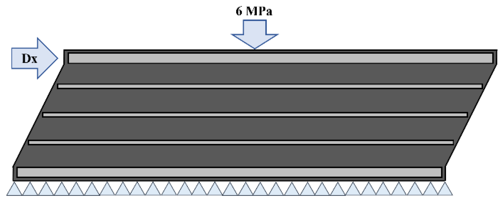
The load and boundary conditions for simulating the shear modulus test method specified in EN 1337-3: Annex F are as follows: All degrees of freedoms of nodes on the bottom of the bearing are fixed and symmetric boundary condition is applied to the symmetry plane. The shear force with respect to shear displacement (Dx) is calculated after moving horizontally from 0 to 100 mm (the shear strain of 0.77) at 10 mm intervals while pressing the upper surface of the bearing with a pressure of 6 MPa. The load and boundary conditions are shown in Figure 7.

3.3. Simulation Results and Discussion

3.3.1. Strength Analysis of Elastomeric Bearing

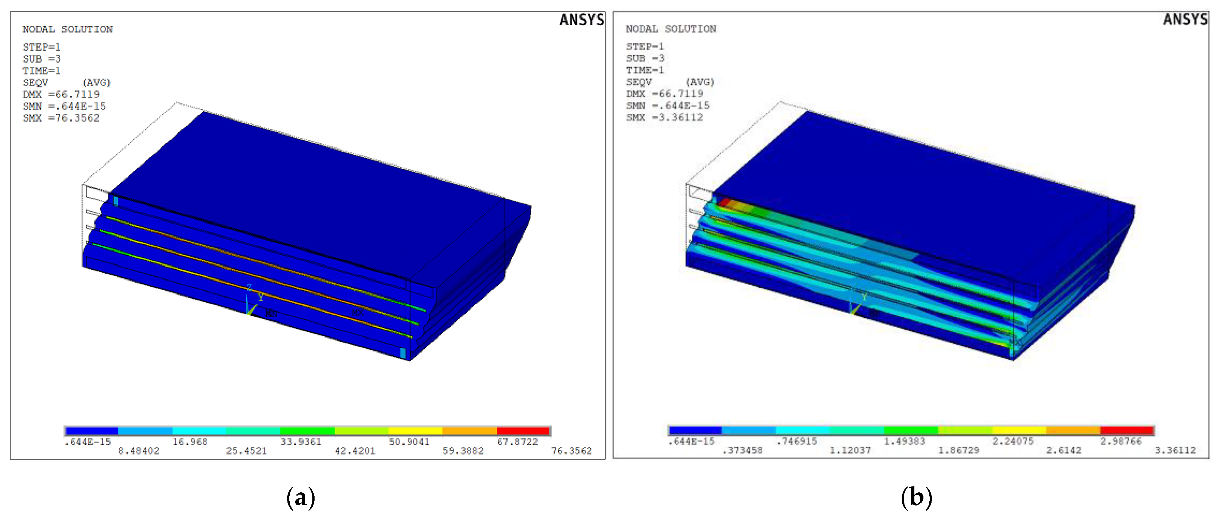
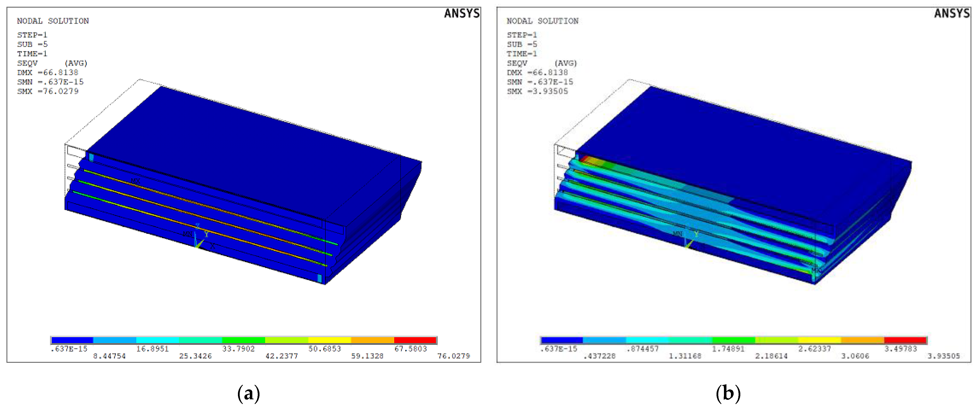
ANSYS Mechanical APDL, a commercial structural analysis software, was used to evaluate the effect of the three nonlinear M-R models (2P, 5P, and 9P) on the shear modulus of the elastomeric bearing. Figure 8, Figure 9 and Figure 10 show the stress distribution with 2P (Figure 8), 5P (Figure 9), and 9P (Figure 10) M-R models when the elastomeric bearing subjected to vertical pressure of 6 MPa (compression) and the shear strain of 0.5 (as shear displacement is 65 mm). The von-Mises stresses (equivalent stress) are plotted, so the values have only positive signs. In Figure 8, Figure 9 and Figure 10, the large equivalent stress of a steel reinforcing plate occurs in the center of the reinforcement plate during compression due to the resistance caused by the chemical bonding between the reinforcing plate and the elastomer. In contrast, the large stress of an elastomer is generated at both ends of the elastomer due to the resistance of the reinforcing plate.
The maximum equivalent stresses and their difference rate of the elastomeric bearing with respect to the three M-R models are shown in Table 6. In Table 6, the difference between stress obtained with 2P and 9P was more than 10 times larger than that between 2P and 5P. This indicates that the 2P and 5P M-R models predict the similar values, and the 9P M-R model predicts a larger value compared with 2P and 5P models. In other words, in the case of compression test, the 9P M-R model has a larger percentage error than other models.

3.3.2. Shear Modulus of Elastomeric Bearing

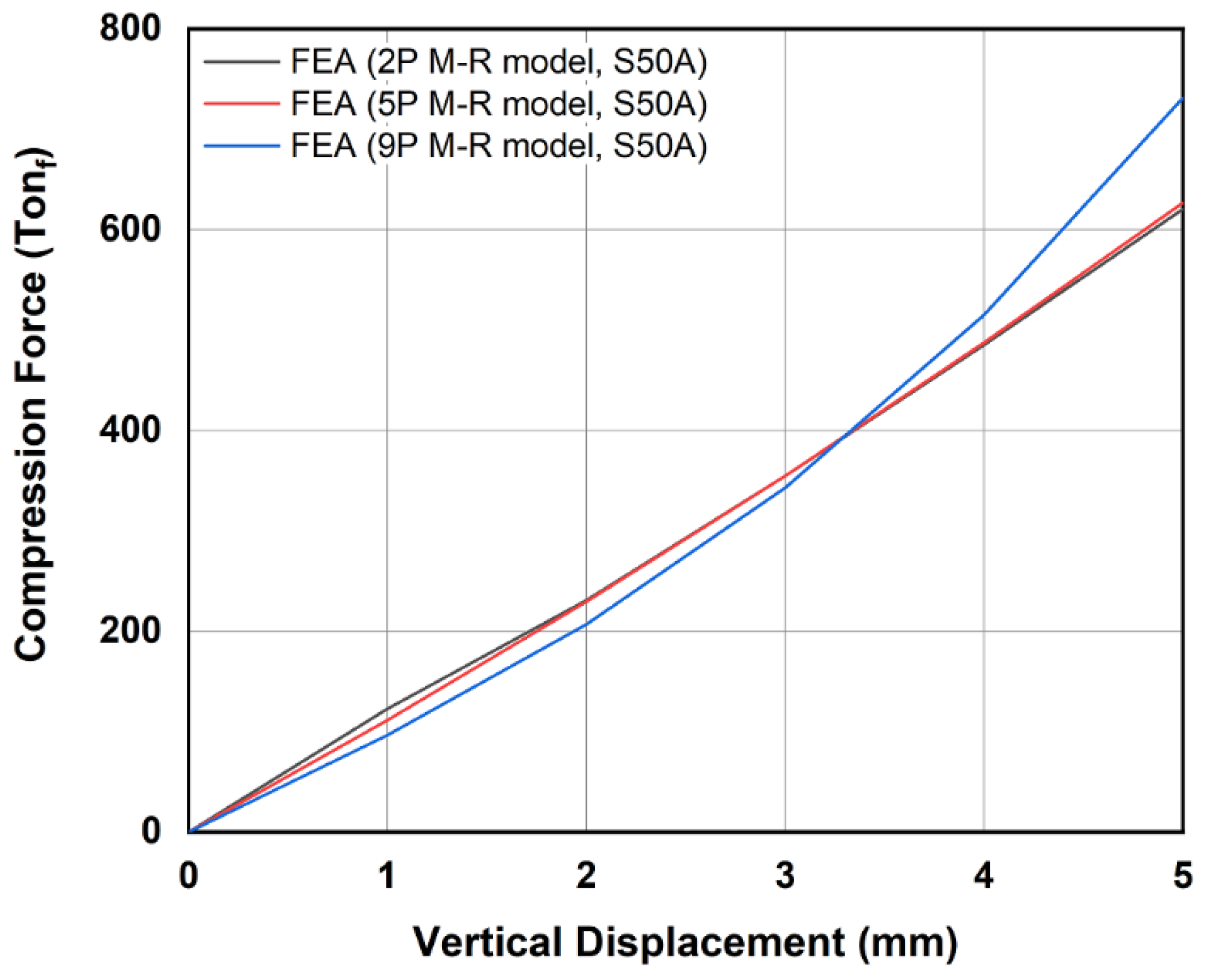
The effect of the three M-R models on the compression and shear of the elastomer bearing was evaluated through the finite element analysis. In order to analyze the effect of three M-R models on the compression of the bearing, the compression forces according to the vertical displacements of the bearing for 2P, 5P, and 9P were found and provided in Table 7. The values of Table 7 are plotted in Figure 11 as the force-displacement graph. Similarly, in order to analyze the effect of three M-R models on the shear of the bearing, the shear force according to the horizontal displacement of the bearing under compression of 392 tonf (corresponding to a pressure of 6 MPa) was found, and the values are provided in Table 8. The values of Table 8 are plotted in Figure 12 as force-displacement graphs. Figure 11 shows the compressive load-displacement graph obtained with the three M-R models. The load-displacement graphs obtained with the 2P and 5P models are almost linear, and the average percentage error between the results obtained with 2P and 5P models is around 2.23% (more details of the error are provided in Table 7), which is negligible. In comparison, we observe a nonlinear trend for the compressive load-displacement graph for the 9P model. The deviation between 2P and 9P model results is around 11.83% (from Table 7), which means that the 9P M-R model is not suitable for simulating compression behavior.
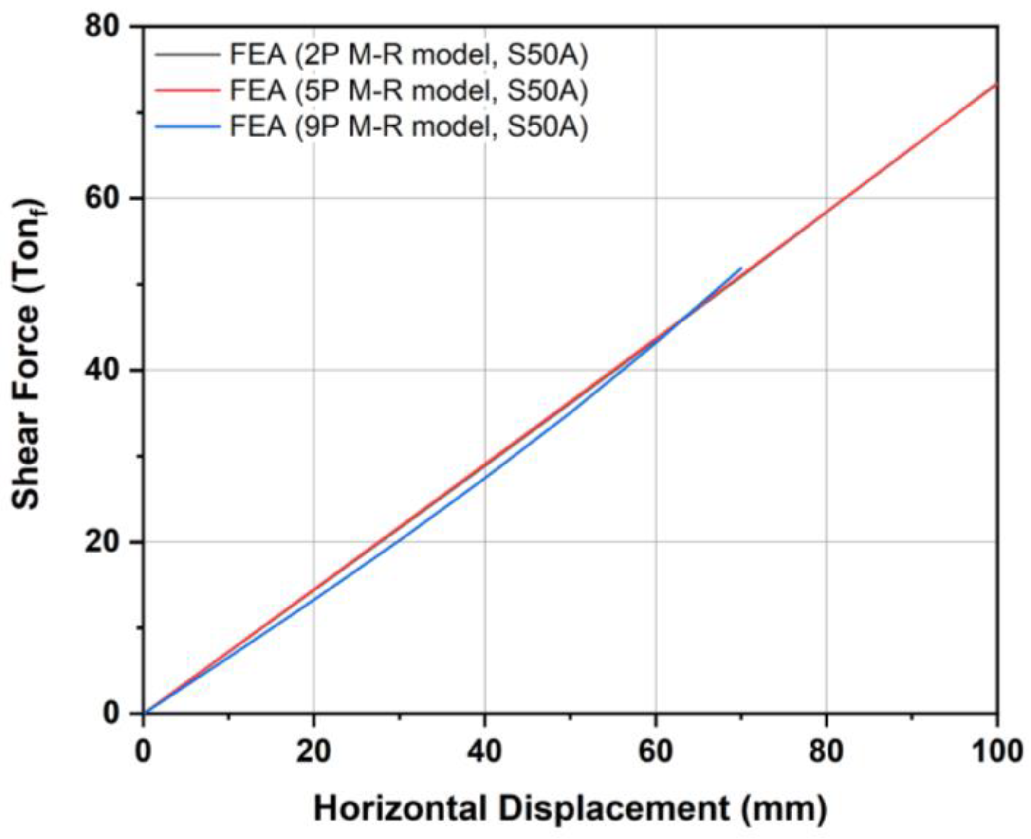
Figure 12 shows the shear force-displacement graph obtained with the three M-R models. All three models almost predict the linear behavior in the shear load, although a slight nonlinear trend is found for the 9P model when the shear strain rate is below 0.5. From Table 8, the deviation between the results of shear force and displacement from 2P and 5P models is almost zero (around 0.38%). On the other hand, the percentage error between 2P and 9P results is nearly about 4.82%. Overall, the third-order 9P M-R model showed a nonlinear curve for both compression and shear load graphs. However, the second-order 5P and the first-order 2P M-R model showed a linear trend for force-displacement graphs with negligible difference between the two results. Therefore, we can say that the 2P M-R model can be successfully applied for simulating the nonlinear behavior of elastomeric bearing under compression and shear loading.

4. Comparing Experimental and Numerical Results

4.1. The Effect of the Number of Elements across an Elastomer Layer

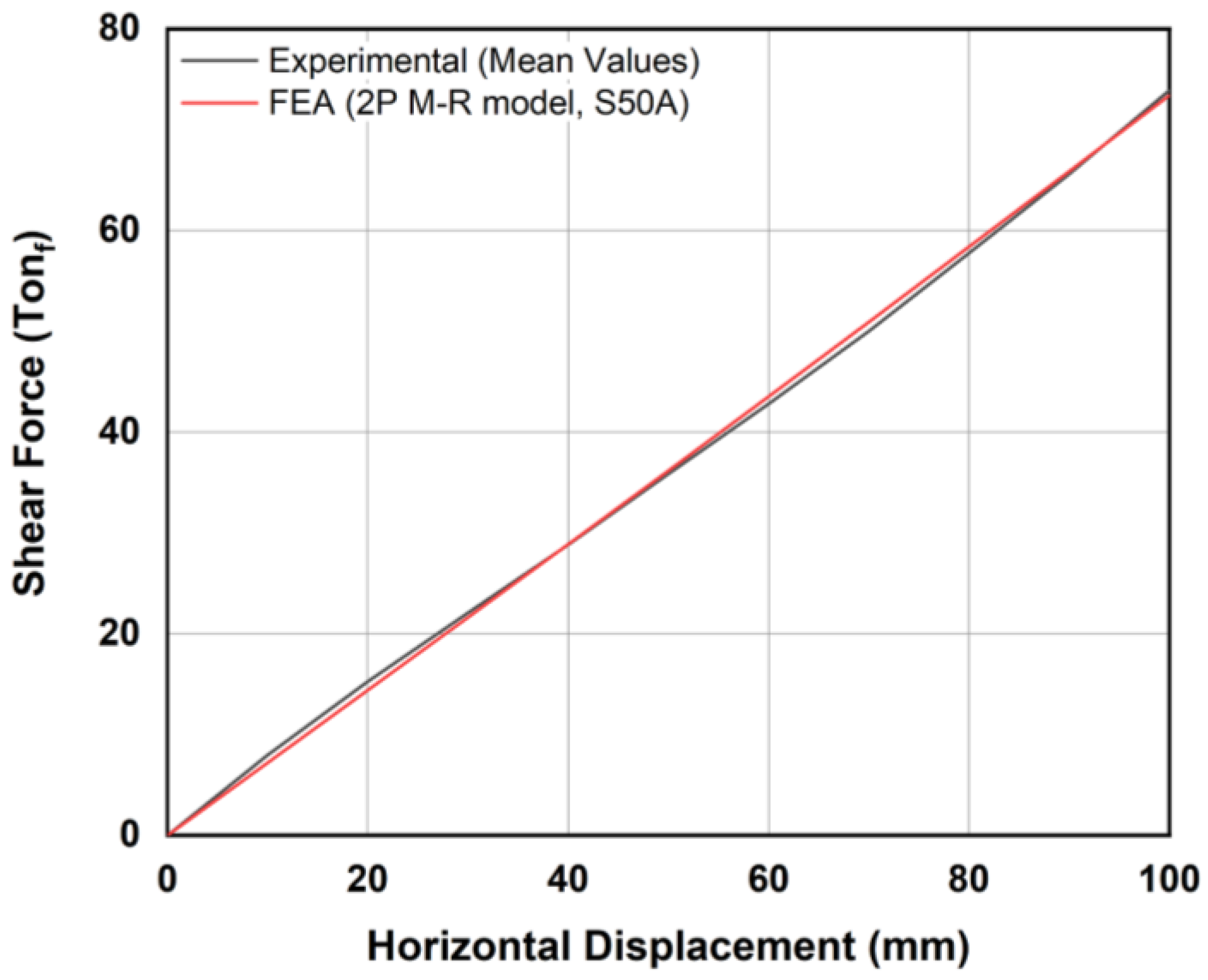
The comparison of the shear force of elastomeric bearing according to the horizontal displacement between the numerical simulation (FEA) and the experiment is shown in Figure 13. The graph in Figure 13 shows that the shear force-displacement graph measured through the experiment changes to a slightly curved shape, whereas the graph calculated through the numerical simulation shows a straight line. This is because the physical properties of the elastomer are defined using the Mooney–Rivlin coefficient in the numerical simulation, while the actual elastomer exhibits nonlinear behavior. However, the difference between the two graphs is negligibly small.
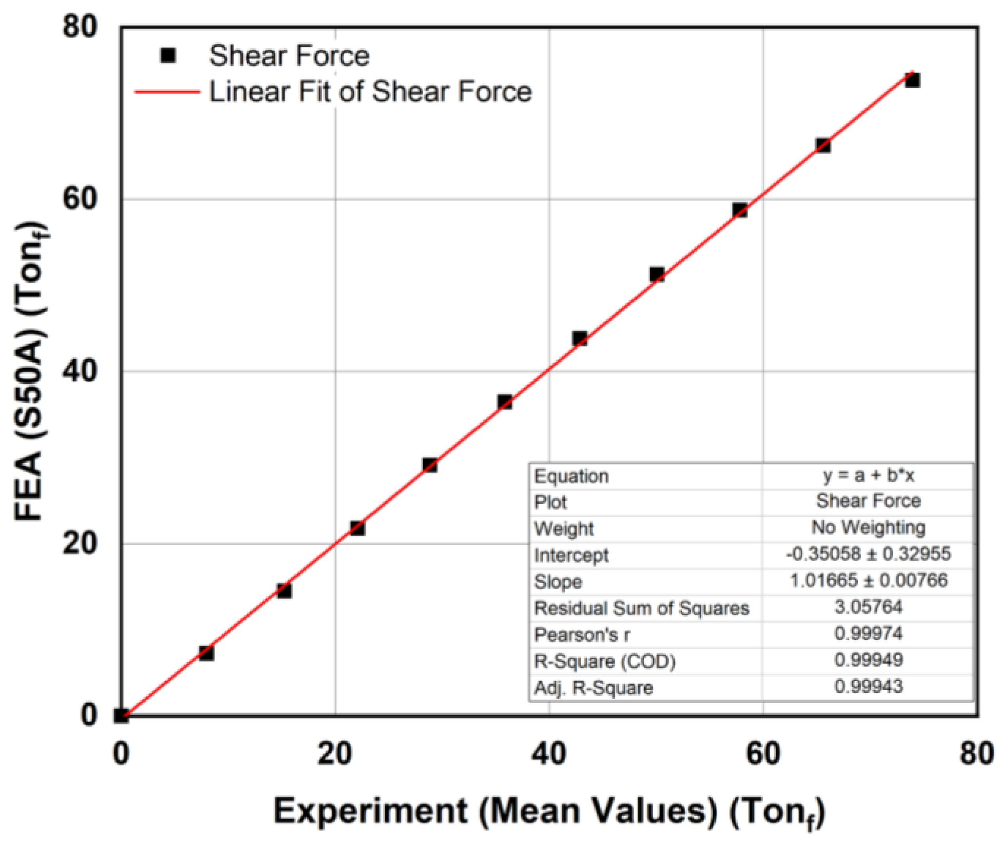
In order to analyze a more quantitative correlation between the experimental and the numerical simulation (at 2P M-R model), a linear fit is performed on the shear force with the horizontal axis as the experiment value and the vertical axis as the FEA value at the shore hardness of 50A; the graph is shown in Figure 14. In Figure 14, the correlation coefficient (R2) for a regression model for the linear relationship between the experiment and the FEA results is 0.99949, indicating a very good fit. It shows that the FEA result of the model with shore hardness of 50A almost corresponds to the experiment result. By comparing the numerical simulation and the experiment result of the elastomeric bearing’s shear modulus, it is confirmed that the finite element analysis conditions for the elastomer bearing are reliable.

4.2. Verification for the Suggested Analysis Conditions

In order to verify the analysis conditions presented in the previous section, the shear force according to the horizontal displacement of the analytical model was obtained through numerical simulations at 60A and 70A as well as the hardness of the elastomer 50A. Table 9 shows the material properties of the elastomer according to the shore hardness.
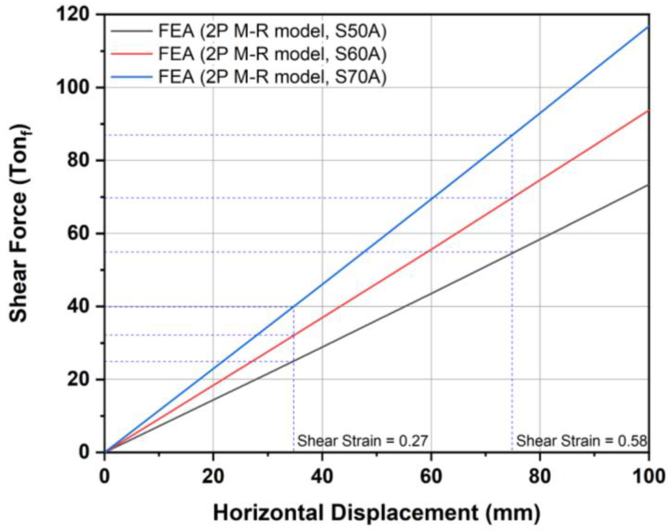
The shear forces according to the horizontal displacement for the elastomeric bearing with 3 types of shore hardness (50A, 60A, and 70A) under compression of 392 tonf (corresponding to a pressure of 6 MPa) was found through the numerical simulation (FEA) when the number of elements across an elastomer layer is 3, and is shown in Table 10. The values of Table 10 are plotted in Figure 15 as force-displacement graphs in order to calculate the shear modulus with respect to the shore hardness of an elastomer. The shear forces of the elastomeric bearing are found at the two deformation points (shear strain of 0.27 and 0.58) of each graph in Figure 15, and the shear modulus is calculated using Equation (1), and the values are represented in Table 11.
In Table 11, the shear modulus of the bearing through the numerical simulation (FEA) is 0.731 MPa (when shore hardness is 50A), 0.935 MPa (when 60A), and 1.165 MPa (when 70A). This indicates that the shear modulus of the bearing through the numerical simulation is corresponding to the values in Table 3: EN 1337-3 Annex D: Shear Modulus Comments. This means that numerical simulations by using Mooney–Rivlin constants in Table 10 as mechanical properties and dividing the number of elements across the elastomer layer by 3 are reliable. It shows that the present numerical modeling can reasonably represent the physical model so that it can repeatedly be used for the design.

5. Conclusions

The most important item when indicating the mechanical properties of offshore elastomeric bearings is the shear modulus, but the experiment incurs a high cost due to a large capacity test equipment and a dedicated shear test device. As an alternative, a method for designing offshore elastomeric bearings through numerical simulation is proposed. In this study, the relationship between the experiment and the numerical simulation on the shear force of the bearing was analyzed to improve the accuracy of the numerical simulation. The conclusions are as follows:
(1) In the experiment according to EN 1337-3 Annex F: Shear Modulus Test, 10 tests for the bearing specimen (800 × 800 × 200 mm) were performed with a shear strain of 0.77 (shear displacement of 100 mm). The measured average shear modulus of the bearing specimen is 0.707 MPa, which corresponds to a Shore A hardness of 50 + 5 grade with reference to EN 1337-3: Annex D.
(2) In the numerical simulation, the Mooney–Rivlin (M-R) model is generally used for the hyperelastic materials, and there are three types of M-R models, such as 2P, 5P, and 9P based on the number of the terms in the series. The results of the compressive load-displacement from 2P and 5P M-R models are almost linear, and the difference between the two values is 2.23% on average, but in the case of 9P model, showing a difference of 11.83% from the 2P model. On the other hand, the shear-force displacement results obtained from the 5P model showed negligible difference with the 2P model, with an average error of 0.38%, and 9P showed an average error of 4.82%. In addition, the correlation coefficient (R2) for a regression model for the linear relationship between the experiment and the numerical simulation (for 2P M-R model) results is 0.99949, indicating a very good fit. Therefore, it can be seen that the nonlinear behavior model suitable for numerical simulation of marine elastomer bearings is the 2P M-R model.
(3) In order to verify the analysis conditions suggested in this study for the numerical simulation, the shear force according to the horizontal displacement of the analytical model was obtained through numerical simulations at 60A and 70A as well as the hardness of the elastomer 50A. The shear modulus of the bearing through the numerical simulation (FEA) is 0.731 MPa (when shore hardness is 50A), 0.935 MPa (when 60A), and 1.165 MPa (when 70A). This indicates that the shear modulus of the bearing through the numerical simulation is corresponding to the values in EN 1337-3 Annex D: Shear Modulus Comments.
(4) Therefore, it is confirmed that the analysis conditions suggested in this study for the numerical simulation of the elastomeric bearing are capable of reproducing the experimental results for the shear modulus.
Author Contributions

Conceptualization, D.H. and W.C.; methodology, D.H. and W.C.; software, D.H.; validation, D.H. and W.C.; formal analysis, D.H. and W.C.; investigation, D.H.; resources, D.H.; data curation, W.C.; writing—original draft preparation, D.H.; writing—review and editing, W.C.; visualization, D.H.; supervision, W.C.; project administration, D.H.; funding acquisition, W.C. All authors have read and agreed to the published version of the manuscript.

Funding

This research received no external funding.

Institutional Review Board Statement

Not applicable.

Informed Consent Statement

Not applicable.

Data Availability Statement

Not applicable.

Acknowledgments

This work was supported by the Dong-A University research fund.

Conflicts of Interest

The authors declare no conflict of interest.

Nomenclature

AArea of elastomeric bearing (B × L)
BBreadth of elastomeric bearing
C1, C10Mooney–Rivlin coefficients
DxHorizontal deformation of elastomeric bearing
DxmMaximum test deflection
EYoung’s modulus
FxHorizontal force (shear force)
FzVertical force (compressive force)
GgConventional shear modulus
LLength of elastomeric bearing
NENumber of elements across an elastomer layer
TqThickness of elastomer
εqx Shear strain
εqx1 Shear strain at a deformation Dx1 = 0.27Tq
εqx2 Shear strain at a deformation Dx2 = 0.58Tq
νPoisson’s ratio
σUUltimate strength
σYYield strength
τs Shear stress
τs1 Shear stress at a deformation Dx1 = 0.27Tq
τs2 Shear stress at a deformation Dx2 = 0.58Tq

References

  1. Abe, M.; Yoshida, J.; Fujino, Y. Multiaxial behaviors of laminated rubber bearings and their modeling I: Experimental study. J. Struct. Eng. 2004, 130, 1119–1132. [Google Scholar] [CrossRef]
  2. Nittmannova, L.; Magura, M. Interaction of reinforced elastomeric bearings in bridge construction. Slovak J. Civ. Eng. 2016, 24, 34–40. [Google Scholar] [CrossRef] [Green Version]
  3. Koo, G.H.; Lee, J.H.; Lee, H.Y.; Yoo, B. Stability of laminated rubber bearing and its application to seismic isolation. KSME Int. J. 1998, 13, 595–604. [Google Scholar] [CrossRef]
  4. Wang, R.Z.; Chen, S.K.; Liu, K.Y.; Wang, C.Y.; Chang, K.C.; Chen, S.H. Analytical simulations of the steel-laminated elastomeric bridge bearing. J. Mech. 2014, 30, 373–382. [Google Scholar] [CrossRef]
  5. Zhao, G.; Ma, Y.; Li, Y.; Luo, J.; Du, C. Development of a modified Mooney-Rivlin constitutive model for rubber to investigate the effects of aging and marine corrosion on seismic isolated bearings. Earthq. Eng. Eng. Vib. 2017, 16, 815–826. [Google Scholar] [CrossRef]
  6. Yang, C.K.; Bae, Y.H.; Kim, M.H.; Ward, E.G. Loads on tie-down systems for floating drilling rigs during hurricane conditions. J. Offshore Polar Eng. 2010, 20, 1–8. [Google Scholar]
  7. Yang, C.K.; Kim, M.H. The structural safety assessment of a tie-down system on a tension leg platform during hurricane events. Int. J. Ocean Syst. Eng. 2011, 1, 263–283. [Google Scholar] [CrossRef]
  8. Hong, S.K.; Lew, J.M.; Jung, D.W.; Kim, H.T.; Lee, D.Y.; Seo, J.S. A study on the impact load acting on an FPSO bow by steep waves. Int. J. Nav. Archit. Ocean Eng. 2017, 9, 1–10. [Google Scholar] [CrossRef] [Green Version]
  9. Lapidaire, P.J.M. The effect of ship motions on FPSO topsides design. Proc. Offshore Technol. Conf. 1996, 28, 411–420. [Google Scholar]
  10. Han, D.S.; Jang, S.H.; Lee, G.H. Stiffness evaluation of elastomeric bearings for leg mating unit. J. Korea Acad. Ind. Coop. Soc. 2017, 18, 106–111. [Google Scholar]
  11. BSi. EN 1337-3:2005 Structural Bearings—Part 3: Elastomeric Bearings; British Standards Institution: London, UK, 2006. [Google Scholar]
  12. Han, D.S.; Kim, M.H. The effect of reinforcing plate on the stiffness of elastomeric bearing for FPSO. Energies 2020, 13, 6640. [Google Scholar] [CrossRef]
  13. Konstantinidis, D.; Kelly, J.M.; Makris, N. Experimental Investigation on the Seismic Response of Bridge Bearings; Report No. EERC 2008-02; Earthquake Earthquake Engineering Research Center, University of California: Berkeley, CA, USA, 2008. [Google Scholar]
  14. Steelman, J.S.; Fahnestock, L.A.; Filipov, E.T.; LaFave, J.M.; Hajjar, J.F.; Fouch, D.A. Shear and friction response of nonseismic laminated elastomeric bridge bearings subject to seismic demands. J. Bridge Eng. 2013, 18, 612–623. [Google Scholar] [CrossRef]
  15. Li, Y.; Wu, Q. Experimental study on friction sliding performance of rubber bearings in bridges. Adv. Mater. Sci. Eng. 2017, 2017, 5845149. [Google Scholar] [CrossRef] [Green Version]
  16. Peng, T.B.; Ni, Y.H.; Wu, Y.C. Real-time substructure tests and numerical simulation of mechanical characteristics of natural rubber-laminated bearings. Strength Mater. 2018, 50, 20–28. [Google Scholar] [CrossRef]
  17. Khaloo, A.; Maghsoudi-Barmi, A.; Moeini, M.E. Numerical parametric investigation of hysteretic behavior of steel-reinforced elastomeric bearings under large shear deformation. Structures 2020, 26, 456–470. [Google Scholar] [CrossRef]
  18. Lee, K.S.; Ki, M.S.; Park, B.J. Comparative study on the nonlinear material model of hyperelastic material due to variations in the streatch ratio. J. Ocean Eng. Technol. 2018, 32, 253–260. [Google Scholar] [CrossRef] [Green Version]
  19. Kumar, N.; Rao, V.V. Hyperelastic Mooney-Rivlin model: Determination and physical interpretation of material constants. Mit Int. J. Mech. Eng. 2016, 6, 43–46. [Google Scholar]
  20. Rao, M.R.; Satayanarayana, M.R.S. On the behavior of hyperelastic materials, a Mooney-Rivlin approach. Int. J. Eng. Res. Technol. 2019, 7, 1–5. [Google Scholar]
  21. ANSYS, Inc. ANSYS Mechanical APDL Material Reference; ANSYS, Inc.: Canonsburg, PA, USA, 2012; pp. 47–57. [Google Scholar]
Figure 1. Shear modulus test conditions.
Applsci 11 04384 g001
Figure 2. Test instruments and shear modulus test of elastomeric bearing specimen: (a) test instrument (2500-ton press and 300-ton horizontal actuator); (b) test specimen; (c) shear deformation of 100 mm (shear strain of 0.77).
Applsci 11 04384 g002
Figure 3. Shear force (red line) and displacement (blue line) graph through performance evaluation (10 times raw test data): (a) test #1; (b) test #2; (c) test #3; (d) test #4; (e) test #5; (f) test #6; (g) test #7; (h) test #8; (i) test #9; (j) test #10.
Applsci 11 04384 g003
Figure 4. Mean shear force-displacement graph of elastomeric bearing specimen measured through the experiment. The thickness of elastomer in this specimen (Tq) is 130 mm.
Applsci 11 04384 g004
Figure 5. Half finite element model of elastomeric bearing (800 × 800 × 200 mm).
Applsci 11 04384 g005
Figure 6. Material behavior curve for the Mooney–Rivlin hyperelastic model.
Applsci 11 04384 g006
Figure 7. Loads and boundary conditions for analysis.
Applsci 11 04384 g007
Figure 8. Stress distribution of elastomeric bearing with 2P M-R model as shear strain is 0.5 under the vertical pressure of 6 MPa: (a) for all domain; (b) for elastomer only.
Applsci 11 04384 g008
Figure 9. Stress distribution of elastomeric bearing with 5P M-R model as shear strain is 0.5 under the vertical pressure of 6 MPa: (a) for all domain; (b) for elastomer only.
Applsci 11 04384 g009
Figure 10. Stress distribution of elastomeric bearing with 9P M-R model as shear strain is 0.5 under the vertical pressure of 6 MPa: (a) for all domain; (b) for elastomer only.
Applsci 11 04384 g010
Figure 11. Compression force-displacement graph with respect to the three M-R models through the numerical simulation.
Applsci 11 04384 g011
Figure 12. Shear force-displacement graph with respect to the three M-R models through the numerical simulation.
Applsci 11 04384 g012
Figure 13. Comparison of shear force-displacement graph between the experiment (mean values of 10 test results) and the numerical simulation (2P M-R model results) at a shore hardness of 50A.
Applsci 11 04384 g013
Figure 14. Correlation of the shear force between the experiment and the FEA when shore hardness of the elastomer is 50A.
Applsci 11 04384 g014
Figure 15. Shear force-displacement graph with respect to the shore hardness of an elastomer through the numerical simulation (FEA). The thickness of elastomer in this specimen (Tq) is 130 mm.
Applsci 11 04384 g015
Table 1. Shear modulus test conditions.
ItemsSpec. ConditionsActual Test Values
Vertical force (pressure)391.8 Tonf * (6 MPa)392.5 Tonf (6.01 MPa)
Shear strain0.7~0.90.77
Test speed150 mm/min138 mm/min
* Tonf stands for Ton-force.
Table 2. Shear modulus test conditions.
εqxDx (mm)Fx (Tonf)Fx (kN)τs (MPa)
0.2735.112.75 (= 25.5/2)125.00.195
0.5875.426.95 (= 53.9/2)264.10.413
Table 3. Shear modulus (Gg) and hardness (Shore A): EN 1337-3 Annex D: Shear Modulus Comments.
Hardness (Shore A)50 + 560 + 570 + 5
Shear modulus (MPa)0.70.91.15
Table 4. Mechanical properties for S355 structural steel (EN 10025-2).
ItemsSignUnitsValues
Young’s modulusEGPa200
Poisson’s ratioν 0.29
Yield strengthσYMPa355
Ultimate strengthσUMPa510~680
Table 5. Mooney–Rivlin constants for neoprene sheet (Shore 50A).
ConstantsUnits2-Parameter5-Parameter9-Parameter
C10MPa0.302−0.0630.590
C01MPa0.0760.436−0.272
C20MPaN/A0.0170.004
C11MPaN/A−0.0140.374
C02MPaN/A−0.003−0.295
C30MPaN/AN/A0
C21MPaN/AN/A−0.107
C12MPaN/AN/A0.109
C03MPaN/AN/A−0.001
D11/MPa000
Table 6. Maximum equivalent stresses and its difference rate of the elastomeric bearing with respect to the Mooney–Rivlin model under compression and shear.
Mooney–Rivlin ModelsSteel PlateElastomer
Stress (MPa)Difference RateStress (MPa)Safety Factor
2-Parameter76.40.0%3.360.0%
5-Parameter76.0−0.5%3.94+17.3%
9-Parameter86.1+12.7%9.16+172.6%
Table 7. Compression force and displacement with respect to the three M-R models through the numerical simulation.
DispacementCompression Forces (Tonf)
(mm)2-Parameter5-Parameter9-Parameter
00.00.00.0
1122.7111.696.4
2231.0229.8207.2
3355.2355.1343.4
4485.3487.8515.3
5620.6627.2731.6
Difference * (%)N/A2.23%11.83%
* Difference (%) is the difference rate between the 5P or 9P value and the 2P value.
Table 8. Shear force and displacement with respect to the number of elements across an elastomer layer (NE) through the numerical simulation (FEA). The thickness of elastomer in this specimen (Tq) is 130 mm.
Dispacement
(mm)
Shear StrainFEA
2-Parameter5-Parameter9-Parameter
000.00.00.0
100.087.37.27.2
200.1514.514.414.4
300.2321.821.621.6
400.3129.128.928.9
500.3836.536.236.2
600.4643.843.543.5
700.5451.350.950.9
800.6258.758.458.4
900.6966.365.965.8
1000.7773.873.473.4
Difference * (%)N/A0.38%4.82%
* Difference (%) is the difference rate between the 5P or 9P value and the 2P value.
Table 9. Mechanical properties for an elastomer according to shore hardness.
ItemsSignUnitValues
S50AS60AS70A
Mooney–Rivlin ConstantsC10MPa0.3020.3820.474
C1MPa0.0760.0960.118
Poisson’s ratioνN/A0.490.490.49
Tensile strengthσUMPa15.015.015.0
Table 10. Shear force and displacement with respect to the shore hardness of an elastomer through the numerical simulation (FEA) when the number of elements across an elastomer layer is 3.
Dispacement
(mm)
Shear StrainShear Forces (Tonf)
S50AS60AS70A
000.00.00.0
100.087.29.211.5
200.1514.418.423.0
300.2321.627.734.5
400.3128.936.946.1
500.3836.246.357.7
600.4643.555.769.4
700.5450.965.181.2
800.6258.474.693.0
900.6965.984.2104.9
1000.7773.493.8116.9
Table 11. Shear forces and shear modulus of the elastomeric bearing with respect to the shore hardness of an elastomer through the numerical simulation (FEA).
Shore Hardnessεqx (N/A)Dx (mm)Fx (Ton)τs (MPa)Gg (MPa)
S50A0.2734.125.340.1940.731
0.5875.454.960.421
S60A0.2734.132.400.2480.935
0.5875.470.230.538
S70A0.2734.140.400.3091.165
0.5875.454.910.670
Publisher’s Note: MDPI stays neutral with regard to jurisdictional claims in published maps and institutional affiliations.