Reducing Motion Blur in Ghost Imaging Via the Hessian Matrix

Abstract

Different from conventional imaging, ghost imaging (GI) is an indirect modality of imaging that needs multiple measurements of the second-order correlation of data collected from two detectors. In some particular cases, the exposure time of two detectors or the rotation speed of the ground glass may not meet the need of experimental condition, resulting in motion blur that reduces the quality of the reconstructed image. In this paper, we propose a method to solve this problem. By convolving the data from the reference arm with the Hessian matrix, the intensity of the light in the data is replaced by the gradient of intensity and the influence of the motion blur in the reconstructed image can be reduced.

1. Introduction

As an indirect modality of imaging, ghost imaging (GI) is a new method of imaging that needs multiple measurements for one imaging process. In the experiment system, the pseudo-thermal light produced by a laser passing through a rotating ground glass (RGG) is split into two arms by a beam splitter (BS); the arm with the illuminated object is called the signal arm and the data without spatial resolution from this arm is recorded by the bucket detector, which means that the data from the detector is the sum of all of the light intensities within the captured range of the detector. The other arm is called the reference arm in which a series of data is recorded by the Complementary Metal Oxide Semiconductor (CMOS) camera [1,2]. After the collection of the data, the image can be reconstructed by some algorithms with data from both arms. When the RGG rotates through the size of the laser spot, the distribution of the laser speckle is gradually changed. Until it rotates out of the entire range of the laser spot, which corresponds to the “coherence time” of the pseudo-thermal light [3], the distribution of the laser speckle could be totally different from the original one. In order to observe the second-order intensity correlation, the coherence time should be close to or shorter than the integration time (exposure time) of the detector in the reference arm, which requires a shorter exposure time or a lower rotation speed of the RGG [4].

Compared with conventional imaging, GI hosts a number of advantages such as high resolution and high sensitivity and could be widely applied in many fields ranging from remote imaging to lidar detection and microscopy [5,6]. The first visualization of GI was realized using entangled photon pairs in 1995 [3] and then it was proved that the experiment could also be realized with pseudo-thermal light sources and even true-thermal light [7,8,9,10]. Recently, modulated light and other types of light sources were applied in an experiment [11,12,13,14]. Due to its convenience in application, the pseudo-thermal source is still commonly used in GI experiments.

In recent years, with the development of ghost imaging, the object is no longer limited to static targets [15,16,17] and different kinds of algorithms and methods have been investigated to deal with the problems in the imaging process with moving objects [18,19]. One of these problems is motion blur, which causes the visual quality decline in the reconstructed image. Due to that, ghost imaging requires multiple samplings in one imaging. The position of the object and speckle should remain relatively static in each acquisition process when it is a moving object, which means a short exposure time and coherence time are needed, leading to the requirement of a fast speed of the RGG and a fast speed of the RGG leads to motion blur.

To overcome this defect, in this paper we introduce the Hessian matrix to compensate for the influence of motion blur caused by the fast speed of the RGG. Based on a table top experimental setup, we measured the image quality of a reconstructed image under different numbers of coincident measurements ranging from under-sampling to over-sampling. The experimental results demonstrated that, with the post-processing method using the Hessian matrix, GI can effectively reconstruct an image with a higher image quality and less influence of motion blur.

2. Materials and Methods

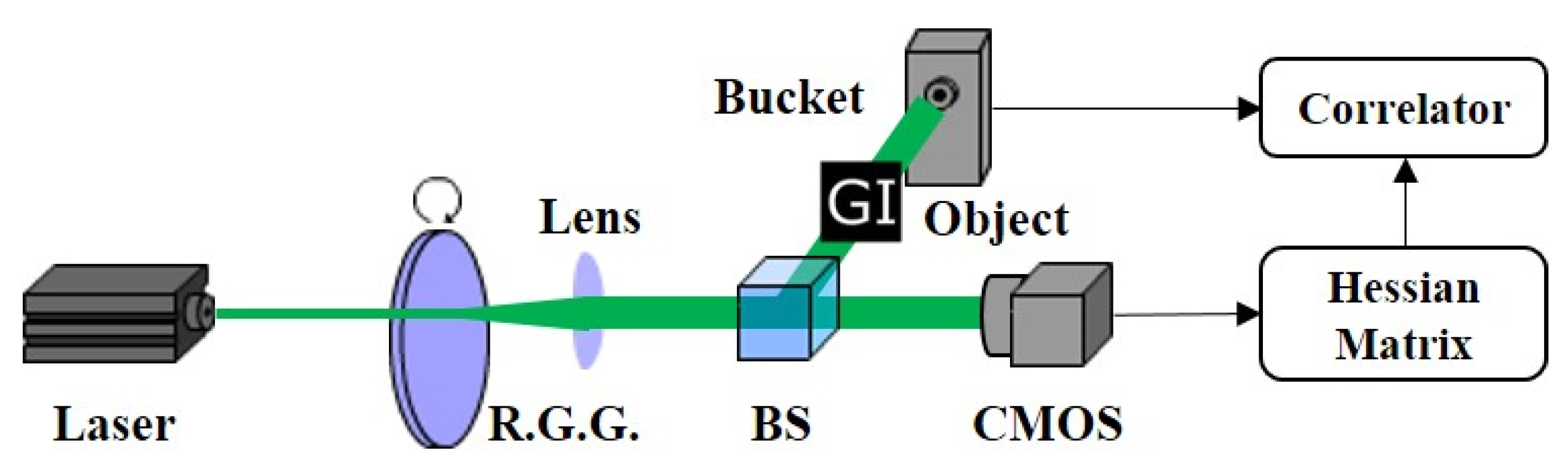
The experimental setup of GI with the Hessian matrix experiment is shown in Figure 1. A 532 nm laser passing through a RGG (Edmund 100 mm diameter 220 grit) made a pseudo-thermal light source. The pseudo-thermal light was split into two arms by a BS. The signal arm penetrated a transitive object (0.3 mm square “GI” pattern) and was summed to be registered by a bucket detector (Thorlabs PDA100/A) while the reference arm, with no object on the path, was recorded by a CMOS camera (xiQ MQ003MG-CM).

In the experiment, we set up the experiment system according to Figure 1 and set the exposure time of the CMOS as 15 ms. Five sets of data were collected including data from the reference arm and the signal arm under different rotation speeds of the RGG, which varied from $\frac{5}{36}$ rad/s to $\frac{25}{36}$ rad/s. The data from the reference arm occupied a field of view of 300 × 300 pixels and the number of samplings in each set of data was 10,000.

The reconstructed image of the object in ghost imaging can be written as [15]:

$$O\left(x,y\right)= \frac{1}{N}{\displaystyle \sum }_{i=1}^N\left(B_i-\langle B\rangle \right)\left(I_i\left(x,y\right)\right)$$

(1)

where $B_i$ was the response of the bucket detector in the $i$th sampling, $\langle B\rangle$ was the ensemble average of $B_i$, $I_i\left(x,y\right)$ was the intensity distribution of the light field recorded by the CMOS camera and N was the number of samplings. Usually, $B_i$ and $I_i\left(x,y\right)$ could be written as the integral of the detectors’ response during the exposure time ${\tau }_e$. This assumes that ${\tau }_e$ is set to be an appropriate value and the reconstructed image has no motion blur. The speed of the RGG was $v_0$ and the speed of the RGG was then set to $v_0+∆v$ for moving object imaging. The speckle field was generated by directing the laser through the RGG and the speckle in the current moment was produced by displacement of it in the previous moment; thus, the faster speed led to a longer distance, which is also called motion blur.

The coherence time could be calculated according Equation (2):

$$\tau =l/\left(\omega \times r\right)$$

(2)

where $\tau$ was the coherence time, $l$ was the diameter of the laser spot, $\omega$ was the angular velocity (RGG) and r was the radius at the laser spot; thus, the coherence time of five sets of data were between 28.64 ms and 5.72 ms (l = 0.5 mm, r = 0.04 m,$\omega$ varied from $\frac{5}{36}$ rad/s to $\frac{25}{36}$ rad/s). In order to mimic the case of motion blur caused by fast speed of the RGG, the camera’s exposure time was set to be 15 ms and the rotation speed of the RGG was set to different values. This made the coherence time vary from less than the exposure time to over the exposure time, which led to a motion blur in both the reference samples and the reconstructed images. We then introduced the Hessian matrix and applied it in the reference samples as a filtering process to get rid of the GI image degradation.

As this is different from the conventional image calculation procedure of GI, before we did the correlation, we first calculated the Hessian matrix of the data in the reference arm. The Hessian matrix can be described as the second-order partial derivative of a matrix [20] and it represents the gradient of the intensity the image. According to the concepts of linear scale-space theory, taking the second-order partial derivative of the image can be written as the convolution of the image and the derivatives of Gaussian functions [21]; thus, Equation (1) can be written as:

$$O^{\prime }\left(x,y\right)= \frac{1}{N}{\displaystyle \sum }_{i=1}^N\left(B_i-\langle B\rangle \right)\left(I_i\left(x,y\right)\otimes \frac{{\partial }^{2}G\left(x,y;\sigma \right)}{\partial x\partial y}\right)$$

(3)

where $\otimes$ is the convolution operator.

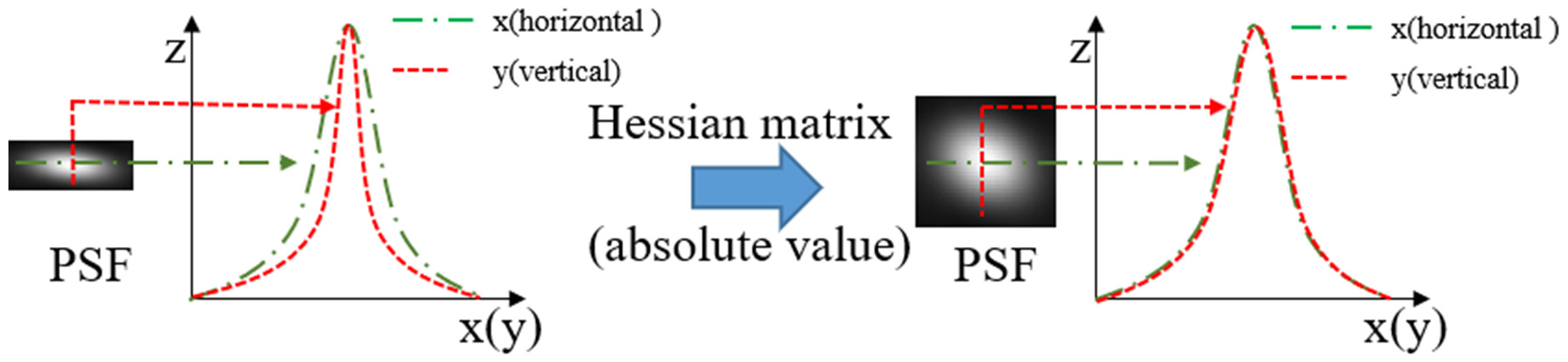
In our method, we first set the value of standard deviation $\sigma$ of the Gaussian function empirically and obtained the convolution window $w$. We then calculated the second-order partial derivative of the Gaussian function, which we think of as the Hessian matrix, then we used the matrix to process the data collected in the reference arm. The data processed by the Hessian matrix were then transferred to compute the correlation with the data from the signal arm instead of the data collected by the CMOS. To state how the Hessian matrix works, we demonstrated the change of the point spread function (PSF) between it being processed by Hessian matrix and not being processed by the Hessian matrix. The PSF of a reconstructed image with motion blur in GI and its projection in the x-z plane and y-z plane is shown in Figure 2. Due to motion blur, the shape of the projection in the x-y plane changed from a circle to an oval. Usually, the projection in the x-z plane and the y-z plane are called a sombrero function. As shown in Figure 3, when we put the sombrero functions into the same coordinates, the difference between the functions was clear. The full width at half maximum (FWHM) of the sombrero function in the x-z plane was larger than that in the y-z plane, which meant that the gradient of the intensity of the sombrero function in the y-z plane dropped faster, leading to a bigger absolute value of the gradient. When the Hessian matrix was introduced to process the data recorded in the reference arm, we actually used the gradient of the intensity instead of the intensity in the data to reconstruct the image. After being filtered by the Hessian matrix, the value of the sombrero function in the y-z plane was increased compared with the function in the z-x plane. This equivalently broadened the FWHM, making the projection in the x-y plane close to a circle; thus, the influence of motion blur was reduced.

3. Results

A brief, related work was published earlier [22]. The results proved that the method worked well when dealing with motion blur. Here, we performed further research. We verified the effect of the method under different rotating speeds of the RGG, compared the method with another deblur algorithm and studied the influence of parameters in our method. Thus, we may provide some reference for others to use this method.

Five groups of data were collected in the experiments. The rotation speed of the RGG was set to $\frac{5}{36 }$ rad/s, $\frac{10 }{36}$ rad/s, $\frac{15 }{36}$ rad/s, $\frac{20}{36}$ rad/s and $\frac{25}{36}$ rad/s and each group was repeated several times in different rotation speeds of the RGG. We used second-order correlation (SC) to reconstruct the images and compared the results with the images reconstructed by SC with the Hessian matrix and the image filtered by the Lucy–Richardson filter [23]. The PSF Lucy–Richardson filter could be calculated during reconstructing the images (as shown in Figure 2a) and the number of iterations in the Lucy–Richardson was set to be 1000. The comparison was implemented on the platform of a MATLAB 2019b with an Intel Core i7-5500U CPU and 12 GB RAM. The computation time of the SC fluctuated between 96 s and 112 s, while the time of the SC with the Hessian matrix increased to about 153 s to 177 s and the time of the SC filtered by the Lucy–Richardson fluctuated between 122 s to 164 s according to the iteration time.

Figure 4 shows the reconstructed image of the Hessian enhanced GI experiment at different rotation speeds of the RGG under 10,000 samplings. As we can see from the figure, compared with the Lucy–Richardson filter, the boundary of the object in the image reconstructed by the SC with the Hessian matrix (II) was much more continuous and clearer, while the noise of the reconstructed images filtered by the Lucy–Richardson filter was much lower. In the condition proposed in the experiment, motion blur was not caused by the moving blur but the high rotational speed of the RGG, making the SC with the Hessian matrix better than the Lucy–Richardson algorithm if we needed a clearer object. When the rotational speed was higher than $\frac{25}{36}$ rad/s, it was almost impossible to reconstruct the image. When the rotational speed was lower than $\frac{5}{36 }$ rad/s, motion blur was no longer an important factor in reducing the image quality.

Taking the third line of data shown in Figure 4 as an example where the rotation speed of the RGG was $\frac{15}{36}$ rad/s, we introduced the signal-to-noise ratio (SNR) to evaluate the performance of the Hessian filter. The SNR can be written as

$$\mathrm{SNR}=10{\log }_{10}\left(\frac{{\sum }_x{\sum }_{y}T{\left(x,y\right)}^2}{{\sum }_x{\sum }_y{\left(O\left(x,y\right)-T\left(x,y\right)\right)}^2}\right)$$

(4)

where $T\left(x,y\right)$ represented the value of the object expected as shown in Figure 5 and $O\left(x,y\right)$ was the reconstructed image.

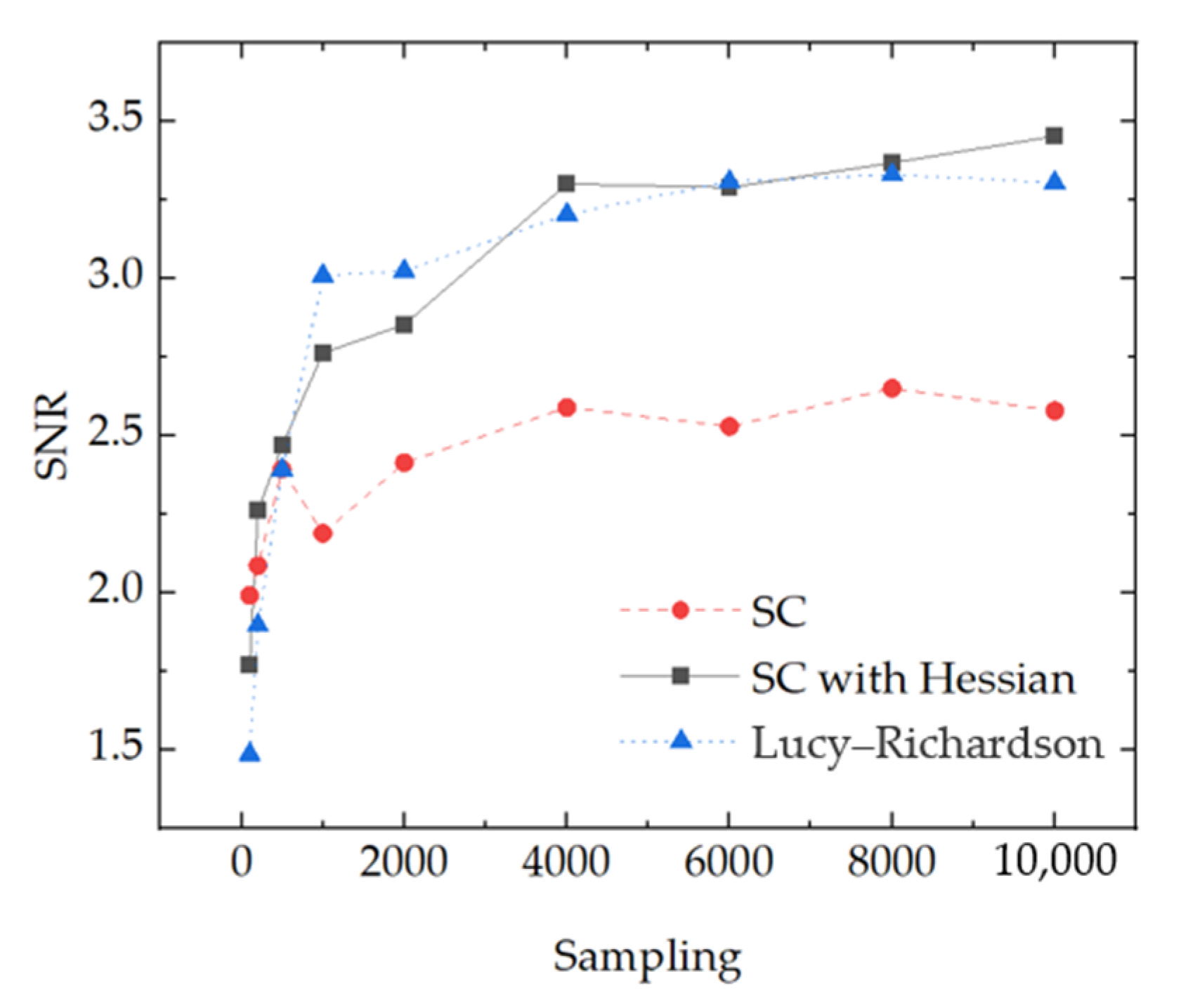
As is shown in Figure 6, the SNR increased as the measurement number increased. When the measurement number was less than 1000, the information in the data collected was not enough to fully reconstruct the image. In contrast, when the measurement number was over 4000, motion blur became an important factor that reduced the image quality. As shown in Figure 4, the Lucy–Richardson filter reduced the noise in the reconstructed images effectively, making the SNR of images reconstructed by SC with the Hessian matrix and those filtered by Lucy–Richardson filter nearly equal.

In addition, it is worth noting that there were two important parameters: the standard deviation $\sigma$ and the convolution window $w$ when calculating the Gaussian second-order partial derivative, which made a big difference to the reconstructed images. The equation between $\sigma$ and $w$ can be written as [24]

$$w=\left(\frac{\sigma -0.8}{0.3}+1\right)\times 2+1$$

(5)

where $w$ determined the range of the pixels where the gradient of intensity was to be calculated; thus, it influenced the performance of the Hessian matrix. In the experiment, the standard deviation $\sigma$ varied from 1 to 5, making the convolution window $w$ vary from 4.3 (considering that the number of pixels is integer and $w$ here was set to be 5) to 31. The reconstructed images of the SC with the Hessian matrix are shown in Figure 7 and Figure 8.

As is shown in Figure 7 and Figure 8, the different value of $\sigma$ led to different reconstructed images. To provide a reference for others to use this method, we studied the relationship between the optimal value of $\sigma$ and the data collected. As the method changed the shape of the PSF from an oval to a circle, we speculated that the optimal value of $\sigma$ related to the ratio of the major axis to the minor axis of the projection in the x-y plane.

As listed in the

Table 1. The ratio and the optimal value of $\sigma$ under different rotational speeds of the RGG.

Rotational Speed of the RGG	Ratio	$\mathbf{Optimal}\mathbf{Value}\mathbf{of}\mathit{\sigma }$
5/36 rad/s	1.5	2
10/36 rad/s	1.8	2
15/36 rad/s	2.1	2
20/36 rad/s	2.4	2
25/36 rad/s	2.9	1

, the ratio of the five sets of data were 1.5, 1.8, 2.1, 2.4 and 2.9 and the optimal value of $\sigma$, as shown in Figure 9, was 2, 2, 2, 2 and 1, respectively. According to the speculation, the optimal value of $\sigma$ should have been 2, 2, 2, 2 and 3. Here we calculated the SNR of five sets of data under different rotational speeds of the RGG and the results are shown in Figure 9. With the exception of the last data group, the optimal of $\sigma$ was about equal to the ratio; thus, our speculation should have been correct. Unfortunately, if the rotational speed of the RGG keeps growing, it is difficult to reconstruct the image no matter what algorithm is used, making it difficult to explore the relationship between the optimal of $\sigma$ and the rotational speed of the RGG further.

4. Discussion

In this paper, we did several experiments to simulate motion blur caused by the improper setting between the exposure time of the detectors and the coherence time. From the experiments, we saw motion blur in the images reconstructed by the SC and SC filtered by Lucy–Richardson, which reduced the quality of reconstructed image. We therefore introduced the Hessian matrix into ghost imaging to reduce the influence caused by motion blur. The results showed that when data were filtered by the Hessian matrix, the reconstructed images had smoother edges, thus improving the quality of the reconstructed images and reducing the influence from motion blur. However, as the cost of the method, when we used the Hessian matrix to deal with motion blur, the resolution was reduced, which may cause some problems if the object has a complex structure. In the further experiments, we hope to find another algorithm to solve the problem that the resolution is reduced when applying the Hessian matrix to the ghost imaging, making the method a promising approach to deal with motion blur in ghost imaging.