Abstract
Recently, deep learning-based defect inspection methods have begun to receive more attention—from both researchers and the industrial community—due to their powerful representation and learning capabilities. These methods, however, require a large number of samples and manual annotation to achieve an acceptable detection rate. In this paper, we propose an unsupervised method of detecting and locating defects on patterned texture surface images which, in the training phase, needs only a moderate number of defect-free samples. An extended deep convolutional generative adversarial network (DCGAN) is utilized to reconstruct input image patches; the resulting residual map can be used to realize the initial segmentation defects. To further improve the accuracy of defect segmentation, a submodule termed “local difference analysis” (LDA) is embedded into the overall module to eliminate false positives. We conduct comparative experiments on a series of datasets and the final results verify the effectiveness of the proposed method.
1. Introduction
Surface defect detection is a hot topic in the field of industrial production, as even small flaws may destroy the appearance of a product [1,2]. As a result, a real-time online process where unqualified products are recognized and discarded or improved is necessary on the production lines in many factories. Traditional methods of achieving this are based mainly on the labor of experienced engineers; these are both time-consuming and costly, and open the process to human error. With the rapid development of computer vision technology, vision-based inspection approaches have, in recent years, gradually come to play an essential role in surface defect detection. As the most representative nondestructive strategy, computer vision-based inspection approaches substitute human eyes and decision-making abilities with optical lenses and intelligent inspection algorithms.
The textures of product surfaces such as textiles, ceramic tiles, steel, etc., can be generally categorized into two groups: patterned (homogeneous) and nonperiodic. Defects on patterned texture surfaces resulting from machine faults or material problems used to be identified as irregularities, and their occurrence can have a harmful effect on product appearance and even performance. To address this, many computer vision-based defect inspection methods have emerged in the last few decades. This remains a challenging strategy, however, for the following reasons: on the one hand, the imaging quality of texture surfaces is easily influenced by certain physical factors (e.g., illumination conditions, shooting angle, sensor errors); on the other, these inspection algorithms have a narrow range of application because of the variety of types of emerging defects (e.g., different scales, varying degrees of contrast with texture background).
To address these problems, a patterned texture surface defect detection method based on background reconstruction and local difference analysis (LDA) is proposed in this paper.
The contributions of this paper are as follows:
- The proposed method uses an unsupervised learning approach in which only defect-free images are used to train the network. This is very meaningful in industrial applications because the occurrence of defective samples is random and unpredictable.
- A novel network which adopts an adversarial learning paradigm is applied to improve reconstruction of the input image.
- A submodule embedded in the whole network is used to implement feature difference analysis, further eliminating false positives. A regional estimation can be drawn from feature analysis based on this module.
This rest of this paper is organized as follows. Section 2 summarizes related work and some classical inspection approaches. In Section 3, our defect detection method is described in detail. Relevant experiments and a discussion are presented in Section 4, and conclusions and limitations are noted in Section 5.
2. Related Works
In this section, we review several representative existing texture surface defect detection methods. These can be divided into two groups: conventional texture analysis-based approaches and deep learning-based approaches.
“Texture analysis” is an umbrella term for a variety of methods based on handcrafted feature extraction and synthesis. It can be further divided into four categories: (i) statistical methods, (ii) structural methods, (iii) spectrum methods, and (iv) model-based methods. Among these, statistical methods and spectrum methods have, to date, proven to be the most practical.
Statistical methods focus on representation forms of spatial distribution of gray values, such as histogram statistics [3,4], autocorrelation functions [5,6], cooccurrence matrices [7], local binary patterns (LBP) [8], and others. Li X. et al. [9] combined spatial gray level cooccurrence matrices with fast discrete curvelet transform to inspect defects on ferrite magnetic tiles, achieving a detection rate of 93.3% with 3.6% false positives.
Structural methods commonly regard the texture model as a composition of texture primitives which are arranged according to certain spatial placement rules; a general pipeline of structural methods is the extraction of texture primitives and inference of arrangement rules in sequence. Tolba and Raafat [10] proposed a multiscale structural similarity index measurement (MS-SSIM) -based method, achieving a 99.1% success rate.
Spectrum methods utilize information from different domains, or synthesize spatial domains and transformed domains, to complete the detection task. Fourier transform (FT) [5,11], wavelet transform (WT) [12,13] and Gabor transform [14,15] are most frequently used approaches in practice. Sari Sarraf and Goddard [16,17] proposed a method combining discrete wavelet transform and edge fusion to segment defects from fabric texture images; they achieved an 89% success rate over 3700 images containing 26 different kinds of defects.
Model-based methods mostly concentrate on the understanding of a random field, which is actually a stochastic modeling under a simple function of an array of random variables. The most famous approaches include the autoregressive model [18,19,20], Markov random fields [21,22], fractal models, and others. Moradi and Zayed [23] used a hidden Markov model to implement a real-time defect detection system for sewer tunnels.
Although the aforementioned texture analysis-based methods have seen much success in past decades, they mainly depend on handcrafted features; this imposes a severe restriction on application range. It is additionally worth mentioning that these methods show extreme sensitivity to illumination consistency and noise influence.
With the rapid development of deep learning technology, computer vision has made breakthroughs in such application fields as object detection, semantic segmentation, target tracking, etc. Recently, research on deep learning-based surface defect detection has attracted a lot of attention, and a variety of relevant studies have been published [24,25,26,27]. Compared with traditional texture analysis methods, deep learning-based methods possess powerful feature representation learning ability and are skilled at solving complex problems. Generally speaking, defect detection methods based on deep learning technology can be categorized into three classes, according to their learning strategies: (i) supervised learning-based methods, (ii) transfer learning-based methods, and (iii) unsupervised learning-based methods.
Supervised learning-based methods are suitable for situations where a number of defect-free and defective samples with reasonable annotations are provided. In [28], the authors proposed a twofold joint detection convolutional neural network (CNN) to automatically extract powerful image features for defect detection on the DAGM (German Association for Pattern Recognition) dataset. In most cases, however, there are not enough samples for model training, and the appearance of faulty products is random; supervised learning-based methods thus impose many restrictive conditions.
Transfer learning can mitigate the problem to a certain extent; it pretrains a model through a common large dataset, then fine-tunes it using specific defective samples. Ren et al. [29] developed a dense prediction model based on a pretrained deep neural network to detect wood texture defects. However, transfer learning-based methods still require a certain amount of labeled sample data, and sometimes show poor success rates because of the mismatching between source domain and target domain.
Unsupervised learning methods do not need any labeled samples at all, which is beneficial for a majority of industry production scenarios. It has been shown that autoencoder (AE) and its variants—convolutional AE (CAE), convolutional denoising AE (CDAE), etc.—are the most successful models, with their distinctive performance of coding and decoding. Mei et al. [30] constructed a Gaussian pyramid-based CDAE architecture for unsupervised learning-based defect inspection, where the Gaussian pyramid is utilized to implement image patch reconstruction and synthesis at different resolutions. They achieved a fair detection success rate over patterned texture images.
Generative adversarial network (GAN) is another kind of unsupervised learning methods to tackle relevant anomaly detection issues, whose primary aim is to produce realistic images. Schlegl et al. [31] proposed a deep convolutional generative adversarial network named AnoGAN to model the manifold of the training data, accompanying a novel reconstruction scheme based on the mapping from image space to a latent space. Hu et al. [32] extended the standard deep convolutional generative adversarial network (DCGAN) by introducing an encoder-like component by which a given query image can be constructed. Then a residual map and a likelihood map can be obtained to realize the detection and localization of surface defects.
3. Proposed Methods
3.1. Basic Principle and Theoretical Foundations
The proposed method is based on the following observation:
Given that a CNN such as CAE, applied to reconstruct the input image, is trainedonly on defect-free images, its reconstruction effectiveness in the defective region of an image will be inferior to that in the defect-free region.
In other words, the corresponding gray level difference between the original and reconstructed images will be larger in the defective region than in the defect-free region. Figure 1a displays a defective surface image of fabric and Figure 1b is a reconstructed version through the proposed CNN. Figure 1c shows the residual map between the above two images and Figure 1d presents the plot of the residual map in 3D perspective. It can be seen from Figure 1 that the discriminative sensitivity in the image reconstruction process can be applied to locate defective regions, and the proposed method follows this principle exactly.
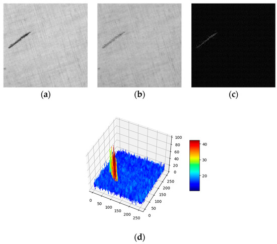
Figure 1.
The different reconstruction effectiveness between defective and defect-free regions. (a) Original image; (b) Reconstructed image; (c) Residual image; (d) 3D heatmap of the residual image.
In general, deep learning-based models employed for image reconstruction are based primarily on CAE. The proposed model uses a similar structure to input and output image data; however, it adopts a different training method, namely, adversarial learning, rather than the conventional method. More specifically, the proposed model is an extended version of DCGAN, which derives from GAN and addresses its training instability through some minor changes. So, to explain our method, it is important to introduce the theoretical foundation of DCGAN.
The primary goal of DCGAN is to generate realistic images. It consists of two CNNs: generator (G) and discriminator (D). The generator maps a latent vector , which usually obeys a specified distribution, to a generated image ; the discriminator maps and the real image sample to a scalar, which is considered as a score ranged [0, 1] to indicate how realistic the input image is. The training phase alternates between two process: (i) the discriminator attaches a high score to and a low one to ; (ii) the generator tries to generate a more realistic image to ‘fool’ the discriminator, from which will get a higher score. The two subnetworks compete with each other during each iteration until the Nash equilibrium of the cost function is reached. Then, in the test phase, the well-trained generator can be used to obtain a realistic image.
The proposed model additionally includes a special feature-based LDA module. Its goal is to cooperate with the residual analysis to obtain a better detection result in the testing phase. As is well-known, the CNN has the ability of representation learning, from which the extracted hierarchical features are more generalized and robust to solve certain vision problems. The proposed method uses this kind of characteristic to locate defects in a region level. Specifically, there is one encoder before and the same encoder after the generator in the DCGAN respectively, which are used to extract the features of the input and reconstructed images; a region-level prediction can then be drawn from the similarity analysis between the two features.
3.2. Architecture of the Model and Training Pipeline
As shown in Figure 2a, the proposed model is composed of four basic CNN components, among which and are similar in structure to an encoder and is a decoder. These encoder-like or decoder-like networks are altogether a series of convolutional blocks. Specifically, for encoder-like and , every block consists of a convolutional layer, a batch normalization layer, and a leaky rectified linear unit (ReLU) layer, except that the first block removes the intermediate batch normalization layer and the last block has only a convolutional layer. The decoder-like is merely a symmetric version of the above two encoders; however, the convolutional layer in each block is replaced by a transposed convolutional layer and the leaky-ReLU layer is substituted by a ReLU layer, except that the last block is a tanh layer. The discriminator is essentially the same as the encoder, but there is a slight variation on the number of channels in the last block, where the discriminator has just one output channel and subsequently attaches a sigmoid layer.
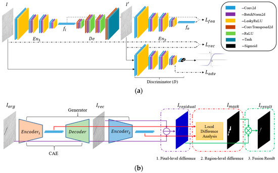
Figure 2.
Overall architecture of the proposed model in the training and testing phases. (a) In the training phase, parameters of the whole network are learned by adversarial learning; (b) In the testing phase, pixel-level and regional-level differences between and are evaluated after image reconstruction to obtain the final segmentaion result.
As mentioned above, the proposed model is trained on defect-free image samples. In practice, a training dataset is composed of many multiscale image patches which are randomly sampled from the different levels of an image pyramid, as shown in Figure 3. Image pyramid is able to adjust the image scale, and here Gaussian pyramid is used to downsample on a whole image. It is based on the fact that defects always take on different sizes, e.g., small dots, thin lines, and even larger areas. Therefore, to completely detect and locate these defects, the model should be trained on multiscale samples. Specifically, a whole image passes through the Gaussian pyramid to generate multiple images whose sizes decrease with the power of two; then, a fixed-size extraction is carried out on these whole images to form ultimate training samples.
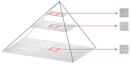
Figure 3.
Gaussian pyramid to extract fixed-size image patches from different scale level.
The object function in the training phase plays an essential role in the final defect detection result, which comprises three optimized objects—, and , respectively—in the proposed model, as shown in Figure 2a.
is designed to improve the quality of image reconstruction through each iteration a, which can be written as:
where and represent the input and reconstructed images and denotes the 1-norm.
is defined as the difference between the extracted features of and , respectively, which can be expressed as:
The introduction of this optimized object is meant to assist in the promotion of image reconstruction quality. Additionally, it is utilized to accomplish the LDA task in the testing phase.
is introduced to guarantee that the reconstructed image be more realistic, which is the primary original goal of the GAN. But unlike DCGAN, the proposed model uses the output of the penultimate CNN block to compare the degree of realism of the input image of the discriminator. The third optimized object can thus be defined as:
where denotes the mapping from the input to the output of penultimate block in the discriminator.
The final loss function is the weighted sum of the above three optimized components as follows:
where , and are all corresponding weighted values summed to 1 and belonging to hyperparameters that need to be adjusted according to the specific dataset.
3.3. Defect Detection and Localization
So long as the proposed model has been trained well, it can be used to determine whether a new image sample is defective or not and, if so, where the defect is located. It should be noted that every CNN other than the discriminator is utilized in the testing phase, as shown in Figure 2b.
Given a pixel-sized texture image, pixel-sized image patches are extracted in sequence where the size is similar to that in the training phase. The well-trained model can then reconstruct each image patch, and all of them are then rearranged to a full-sized reconstructed image. Next, a pixel-level comparison is conducted upon the input and reconstructed images, which can be expressed as:
where denotes the result of the pixel-level difference which is termed residual image and represents the absolute value operation.
Besides the reconstruction use case, the proposed model is also employed to implement LDA. Figure 4b depicts the final detection result which is directly derived from the residual image; it contains some sparkles. In fact, such inferences often appear in the borders of texture patterns, and noise points can also be misjudged as defects. Generally, the gray values of these areas are higher than those of the true defect regions. As a result, a relatively precise localization of defect can be realized only by a pixel-level difference. Figure 4c displays the detection result with local difference analysis (LDA), where previous sparkles are eliminated. The LDA module therefore plays an important role in the localization of defects.
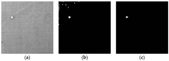
Figure 4.
The comparison between methods with and without local difference analysis (LDA) module. (a) Original image; (b) The final detection result without LDA; (c) The final detection result with LDA.
In the testing phase, two feature vectors are obtained, which are powerful feature representations with respect to the input and reconstructed image patches. The reconstructed version of a defective image patch shows lower sensitivity in abnormal regions, so there are apparent differences between their corresponding features. For a defect-free image patch, the opposite is true. A similarity analysis can thus be carried out between the two feature vectors, through which the probability of defect occurrence can be acquired. The above description can be formulated as follows:
where , and . and denote the size of the whole image and the image patch, respectively. The top-right corner represents the appointed image patch in the mask image . denotes the feature vector for the original image , as does for the reconstructed image . is a threshold to control the sensitivity of being evaluated as a defective region. All mask patches are then rearranged to form a full-sized mask image . The first row in Figure 5 displays four defective images with different texture background; the second demonstrates four corresponding mask images through which regional-level rough defect localization can be accomplished.
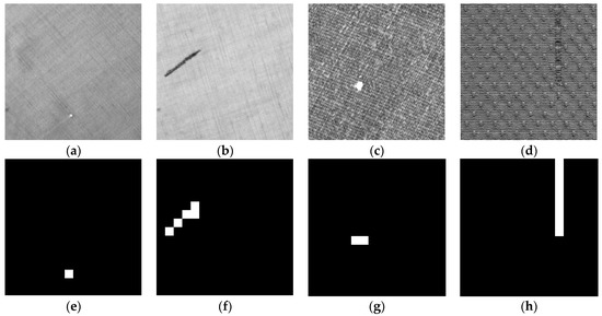
Figure 5.
The effectiveness of local difference analysis. (a–d) The defective images; (e–h) The mask images corresponding to (a–d).
Together with the residual image and mask image, a fusion strategy is put into effect to synthesize them and obtain the final detection result. The process can be formulated as:
where denotes the element-wise multiplication operation (Hadamard product) and and represent the mean and standard deviation of the residual image respectively.
The entire preceding discussion can be summarized the following Algorithm 1:
| Algorithm 1. The defect detection and segmentation. |
| Input: A defective image , well-trained CovNets submodules , and . |
| Output: The final segmentation result |
| Split the input image into a batch of image patches without overlapping area which can be denoted as , and . |
| Obtain the reconstructed image patches and two corresponding feature vectors and . |
| Rearrange into a full-sized reconstructed image and obtain the residual image through Equation (5). |
| Compare the similarity value between and to generate the mask image patches . |
| Rearrange and obtain a full-sized mask image with a threshold value as shown in Equation (6). |
| Synthesize and to obtain the final segmentation image through Equation (7). |
4. Experiments and Discussion
In this section, we detail several experiments we conducted to evaluate the performance of the proposed defect detection method both qualitatively and quantitatively. First, experimental data and parameter configuration are briefly described. Second, the effectiveness of the local difference module is shown. Finally, the inspection performance of the proposed method is compared with that of several other unsupervised methods.
4.1. Dataset Description and Implementation Details
The dataset used in our experiment is composed of TILDA Textile Texture [33], Patterned Fabric [34,35] and MVTec Anomaly Detection [36]. The first contains six kinds of texture images, with 50 defect-free images in each category. The second includes three kinds of texture pattern—namely box, dot, and star—each with 25 to 30 defect-free samples and defective samples which can be utilized as training dataset and testing dataset respectively. The last contains over 5000 high-resolution images divided into fifteen different object and texture categories, each with a set of defect-free training images and a test set of images with various kinds of defects. We totally selected ten kinds of texture background and constructed ten datasets accordingly, where four from the first (c1, c2, c3 and c5), there from the second (box, dot and star) and three from the last (leather, tile and wood).
As described in Section 3.2, the proposed method is composed of four submodules: two encoders and , one decoder , and a discriminator . The detailed parameter setup is depicted in Table 1 and Table 2.

Table 1.
The parameter configuration of the proposed model on submodules , and .
Table 2.
The parameter configuration of the proposed model on submodule .
To further evaluate the performance of the proposed method, a quantitative analysis based on the following three indicators was undertaken.
where TP represents the number of correctly detected defect pixels, FP denotes the number of falsely detected defect pixels and FN is the number of falsely detected background pixels. F1-Measure is a more convincing indicator, taking precision and recall into account. All three of these indicators are ranged [0, 1]; the higher the value, the better the performance.
The proposed method was implemented on a desktop computer with six cores, 16 GB memory, and a GTX 1660 Nvidia GPU. The code was implemented using Python 3.7 with packages Pytorch, Numpy, and OpenCV.
4.2. Local Difference Analysis Module
As mentioned in Section 3.3, the LDA module can effectively improve the accuracy of defect segmentation. It can remove falsely detected background regions by feature analysis. Figure 6 exhibits its special effect in detail, while Table 3 records the comparative quantitative results of methods with and without LDA.
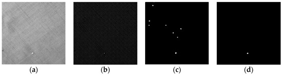
Figure 6.
The influence of the local difference analysis module. (a) Original image; (b) Residual image; (c) Segmentation result only with morphological operation; (d) Segmentation with LDA.
Table 3.
Results of different detection methods.
The first method directly adopts morphological operation on the residual image. Even so, there were many falsely detected regions, and low quantitative indicators were drawn. The second method applied LDA, i.e., it removed almost all of the interfering factors. This is reflected by the fact that all three indicators increased by some degree.
4.3. Comparative Experiments of Different Methods
In order to evaluate the effectiveness of our method, we carried out comparative experiments between the proposed method and three other unsupervised methods: PHOT [37], AnoGAN [31] and MSCDAE [30]. All methods were trained and tested with the same dataset. The inspection results over eight different kinds of texture sample are illustrated in Figure 7, Figure 8 and Figure 9.
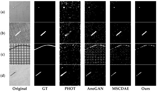
Figure 7.
Segmentation results of defective samples with four kinds of textural background from TILDA Textile Texture dataset under different methods. Each row from left to right are original defect image, ground truth image, results derived from PHOT, AnoGAN, MSCDAE, and our methods. (a) c1; (b) c2; (c) c3; (d) c5.
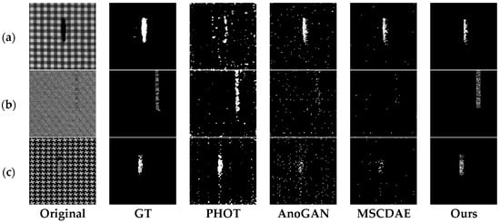
Figure 8.
Segmentation results of defective samples with three kinds of textural background from Patterned Fabric dataset under different methods. Each row from left to right are original defect image, ground truth image, results derived from PHOT, AnoGAN, MSCDAE, and our methods. (a) box; (b) dot; (c) star.
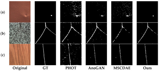
Figure 9.
Segmentation results of defective samples with three kinds of textural background from MVTec Anomaly Detection dataset under different methods. Each row from left to right are original defect image, ground truth image, results derived from PHOT, AnoGAN, MSCDAE, and our methods. (a) leather; (b) tile; (c) wood.
The PHOT method is based on an observation in the Fourier representation of signals where spectral phase can retain many important features of original signals; this does not work for spectral magnitude. The PHOT method always introduces a high alarm rate because of the global reconstruction scheme (Figure 7a,c, Figure 8a and Figure 9a). The second method, AnoGAN, applies generative adversarial network to model the manifold of the defect-free samples and an inverse mapping from image space to latent space is conducted to generate the corresponding reconstructed image for a given query sample. Then a pixel-level comparison is used to realize segmentation of anomaly area. It does not consider the spatial dependencies among pixels and achieves a considerably high false positive rate, as shown in Figure 7c, Figure 8b and Figure 9a. The third method, MSCDAE, is another deep learning-based method, but its basic component is convolutional autoencoder. Its reconstruction ability is realized through CDAE and a Gaussian pyramid is introduced to improve the robustness of the final inspection result. The MSCDAE method exhibits good performance in images where there is a great difference in gray level between defect and background, as shown in Figure 7a,b,d, Figure 8a and Figure 9c, but performs poorly in Figure 8b,c due to the imperfect reconstruction ability of CAE. In contrast to the above three, our method employs adversarial learning to enhance image reconstruction ability, and introduces a regional analysis module to reduce the false positive rate. It showed superior performance in almost all images, as shown in the last row from Figure 7, Figure 8 and Figure 9.
The quantitative inspection results of the four methods are exhibited in Table 4, Table 5 and Table 6, where the bold data indicates better results. It can be seen that the previous three methods always fail in some cases. Specifically, the PHOT method has comparably low F1-measure values in Figure 7a–c and Figure 8a; its global reconstruction strategy resulted in many falsely detected regions. The AnoGAN method has very low precision values in almost all cases, because it merely adopts a global reconstruction scheme and ignores the space connection. The MSCDAE method could hardly segment defects in Figure 8b,c because of its poor reconstruction ability over complex texture images.
Table 4.
Quantitative comparative results of Figure 7a–d between different methods.
Table 5.
Quantitative comparative results of Figure 8a–c between different methods.
Table 6.
Quantitative comparative results of Figure 9a–c between different methods.
The proposed method achieved superior segmentation performance in almost every test. The reasons for this can be summarized in the following two points: firstly, the adversarial learning-based training strategy can improve the ability of image reconstruction; second, the regional analysis module can remove a majority of falsely detected background regions.
5. Conclusions
In this paper, we propose an unsupervised learning-based method to detect and segment defects in texture images. A novel model based on a deep convolutional generative adversarial network (DCGAN) is utilized to reconstruct the input image; the obtained residual image is utilized to predict the position of defect at a global view. An embedded local difference analysis module is presented to locate defects at the regional level, which can eliminate falsely detected areas. Finally, the pixel-level and regional-level predictions are synthesized to obtain the final result. A series of comparative experiments were conducted and confirmed that the proposed method is effective and has a wide range of applications.
Our method showed superior performance with a wide range of texture surfaces. Yet, there are still difficulties in detecting some confusing defects which have a high degree of similarity with texture background in appearance. In the future, we would like to explore some machine learning-based strategies to improve the distinctiveness between foreground and background areas.
Author Contributions
Conceptualization, J.W. and Y.W.; methodology, J.W., G.Y. and S.Z.; validation, J.W. and Y.W.; formal analysis, J.W., G.Y., S.Z. and Y.W.; writing—original draft preparation, J.W., G.Y. and S.Z.; writing—review and editing, J.W., G.Y. and S.Z. All authors have read and agreed to the published version of the manuscript.
Funding
This research was funded by the National Natural Science Foundation of China, grant number 51875515 and the Science and Technology Program of Beijing, grant number Z191100001419014.
Institutional Review Board Statement
No applicable.
Informed Consent Statement
No applicable.
Data Availability Statement
The data presented in this study are openly available and referenced in the References section.
Conflicts of Interest
The authors declare no conflict of interest.
References
- Czimmermann, T.; Ciuti, G.; Milazzo, M.; Chiurazzi, M.; Roccella, S.; Oddo, C.M.; Dario, P. Visual-Based Defect Detection and Classification Approaches for Industrial Applications—A survey. Sensors 2020, 20, 1459. [Google Scholar] [CrossRef] [PubMed]
- Ngan, H.Y.T.; Pang, G.K.H.; Yung, N.H.C. Automated fabric defect detection—A review. Image Vis. Comput. 2011, 29, 442–458. [Google Scholar] [CrossRef]
- Yuan, X.-C.; Wu, L.-S.; Peng, Q. An improved Otsu method using the weighted object variance for defect detection. Appl. Surf. Sci. 2015, 349, 472–484. [Google Scholar] [CrossRef]
- Aminzadeh, M.; Kurfess, T. Automatic thresholding for defect detection by background histogram mode extents. J. Manuf. Syst. 2015, 37, 83–92. [Google Scholar] [CrossRef]
- Wood, E.J. Applying fourier and associated transforms to pattern characterization in textiles. Text. Res. J. 1990, 60, 212–220. [Google Scholar] [CrossRef]
- Haralick, R.M. Statistical and structural approaches to texture. Proc. IEEE 1979, 67, 786–804. [Google Scholar] [CrossRef]
- Haralick, R.M.; Shanmugam, K.; Dinstein, I. Textural Features for Image Classification. IEEE Trans. Syst. Man Cybern. Syst. 1973, 3, 610–621. [Google Scholar] [CrossRef]
- Ojala, T.; Pietikäinen, M.; Harwood, D. A comparative study of texture measures with classification based on featured distributions. Pattern Recognit. 1996, 29, 51–59. [Google Scholar] [CrossRef]
- Li, X.; Jiang, H.; Yin, G. Detection of surface crack defects on ferrite magnetic tile. NDT&E Int. 2014, 62, 6–13. [Google Scholar]
- Tolba, A.S.; Raafat, H.M. Multiscale image quality measures for defect detection in thin films. Int. J. Adv. Manuf. Technol. 2015, 79, 113–122. [Google Scholar] [CrossRef]
- Hoffer, L.; Francini, F.; Tiribilli, B.; Longobardi, G. Neural networks for the optical recognition of defects in cloth. Opt. Eng. 1996, 35, 3183–3190. [Google Scholar] [CrossRef]
- Yang, X.; Pang, G.; Yung, N. Discriminative fabric defect detection using adaptive wavelets. Opt. Eng. 2002, 41, 3116–3126. [Google Scholar] [CrossRef]
- Karayiannis, Y.A.; Stojanovic, R.; Mitropoulos, P.; Koulamas, C.; Stouraitis, T.; Koubias, S.; Papadopoulos, G. Defect detection and classification on web textile fabric using multiresolution decomposition and neural networks. In Proceedings of the IEEE International Conference on Electronics, Circuits and Systems, Pafos, Cyprus, 5–8 September 1999; pp. 765–768. [Google Scholar]
- Ogata, N.; Fukuma, S.; Nishikado, H.; Shirosaki, A.; Takagi, S.; Sakurai, T. An accurate inspection of PDP-mesh cloth using Gabor filter. In Proceedings of the International Symposium on Intelligent Signal Processing and Communication Systems, Hong Kong, China, 13–16 December 2005; pp. 65–68. [Google Scholar]
- Mak, K.L.; Peng, P. An automated inspection system for textile fabrics based on Gabor filters. Robot. Comput. Integr. Manuf. 2008, 24, 359–369. [Google Scholar] [CrossRef]
- Sari-Sarraf, H.; Goddard, J.S. Vision system for on-loom fabric inspection. In Proceedings of the Textile, Fiber & Film Industry Technical Conference, Charlotte, NC, USA, 5–7 May 1999; pp. 1252–1259. [Google Scholar]
- Sari-Sarraf, H.; Goddard, J.S. Robust defect segmentation in woven fabrics. In Proceedings of the IEEE Computer Society Conference on Computer Vision and Pattern Recognition, Santa Barbara, CA, USA, 25–25 June 1998; pp. 938–944. [Google Scholar]
- Serafim, A.L. Segmentation of natural images based on multiresolution pyramids linking of the parameters of an autoregressive rotation invariant model. Application to leather defects detection. In Proceedings of the International Conference on Pattern Recognition, Conference C: Image, Speech & Signal Analysis, The Hague, The Netherlands, 30 August–1 September 1992; pp. 41–44. [Google Scholar]
- Serafim, A.F.L. Multiresolution pyramids for segmentation of natural images based on autoregressive models: Application to calf leather classification. In Proceedings of the International Conference on Industrial Electronics, Control and Instrumentation, Kobe, Japan, 28 October–1 November 1991; pp. 1842–1847. [Google Scholar]
- Alata, O.; Ramananjarasoa, C. Unsupervised textured image segmentation using 2-D quarter plane autoregressive model with four prediction supports. Pattern Recognit. Lett. 2005, 26, 1069–1081. [Google Scholar] [CrossRef]
- Ozdemir, S.; Ercil, A. Markov random fields and Karhunen-Loeve transforms for defect inspection of textile products. In Proceedings of the IEEE Conference on Emerging Technologies and Factory Automation, Kauai, HI, USA, 18–21 November 1996; pp. 697–703. [Google Scholar]
- Cohen, F.S.; Fan, Z.; Attali, S. Automated inspection of textile fabrics using textural models. IEEE Trans. Pattern Anal. Mach. Intell. 1991, 13, 803–808. [Google Scholar] [CrossRef]
- Moradi, S.; Zayed, T. Real-time defect detection in sewer closed circuit television inspection videos. In Pipelines 2017; ASCE: Reston, VA, USA, 2017; pp. 295–307. [Google Scholar]
- Psuj, G. Multi-Sensor Data Integration Using Deep Learning for Characterization of Defects in Steel Elements. Sensors 2018, 18, 292. [Google Scholar] [CrossRef]
- Gopalakrishnan, K.; Khaitan, S.K.; Choudhary, A.; Agrawal, A. Deep Convolutional Neural Networks with transfer learning for computer vision-based data-driven pavement distress detection. Constr. Build. Mater. 2017, 157, 322–330. [Google Scholar] [CrossRef]
- Lin, H.; Li, B.; Wang, X.; Shu, Y.; Niu, S. Automated defect inspection of LED chip using deep convolutional neural network. J. Intell. Manuf. 2019, 30, 2525–2534. [Google Scholar] [CrossRef]
- Tabernik, D.; Šela, S.; Skvarč, J.; Skočaj, D. Segmentation-based deep-learning approach for surface-defect detection. J. Intell. Manuf. 2020, 31, 759–776. [Google Scholar] [CrossRef]
- Wang, T.; Chen, Y.; Qiao, M.; Snoussi, H. A fast and robust convolutional neural network-based defect detection model in product quality control. Int. J. Adv. Manuf. Technol. 2018, 94, 3465–3471. [Google Scholar] [CrossRef]
- Ren, R.; Hung, T.; Tan, K.C. A Generic Deep-Learning-Based Approach for Automated Surface Inspection. IEEE Trans. Cybern. 2018, 48, 929–940. [Google Scholar] [CrossRef] [PubMed]
- Mei, S.; Yang, H.; Yin, Z. An Unsupervised-Learning-Based Approach for Automated Defect Inspection on Textured Surfaces. IEEE Trans. Instrum. Meas. 2018, 67, 1266–1277. [Google Scholar] [CrossRef]
- Schlegl, T.; Seebck, P.; Waldstein, S.M.; Schmidt-Erfurth, U.; Langs, G. Unsupervised Anomaly Detection with Generative Adversarial Networks to Guide Marker Discovery. In Proceedings of the International Conference on Information Processing in Medical Imaging, Boone, NC, USA, 25–30 June 2017; pp. 146–157. [Google Scholar]
- Hu, G.; Huang, J.; Wang, Q.; Li, J.; Xu, Z.; Huang, X. Unsupervised fabric defect detection based on a deep convolutional generative adversarial network. Text. Res. J. 2019, 90, 247–270. [Google Scholar] [CrossRef]
- TILDA Textile Texture Database. Available online: https://lmb.informatik.uni-freiburg.de/resources/datasets/tilda.en.html (accessed on 18 December 2020).
- Ng, M.K.; Ngan, H.Y.T.; Yuan, X.; Zhang, W. Patterned Fabric Inspection and Visualization by the Method of Image Decomposition. IEEE Trans. Autom. Sci. Eng. 2014, 11, 943–947. [Google Scholar] [CrossRef]
- Ngan, H.Y.T.; Pang, G.K.H. Regularity Analysis for Patterned Texture Inspection. IEEE Trans. Autom. Sci. Eng. 2009, 6, 131–144. [Google Scholar] [CrossRef]
- Bergmann, P.; Fauser, M.; Sattlegger, D.; Steger, C. MVTec AD—A Comprehensive Real-World Dataset for Unsupervised Anomaly Detection. In Proceedings of the IEEE Conference on Computer Vision and Pattern Recognition, Long Beach, CA, USA, 15–20 June 2019; pp. 9584–9592. [Google Scholar]
- Aiger, D.; Talbot, H. The phase only transform for unsupervised surface defect detection. In Emerging Topics in Computer Vision and Its Applications; World Scientific Pub. Co.: Singapore, 2010; pp. 215–232. [Google Scholar]
Publisher’s Note: MDPI stays neutral with regard to jurisdictional claims in published maps and institutional affiliations. |
© 2020 by the authors. Licensee MDPI, Basel, Switzerland. This article is an open access article distributed under the terms and conditions of the Creative Commons Attribution (CC BY) license (http://creativecommons.org/licenses/by/4.0/).