Influence of Model and Traffic Pattern on Determining the Self-Similarity in IP Networks

Abstract

This study aimed to determine the applicability of using selected libraries of computing environment R to establish the coefficient of self-similarity. R environment is an analytical environment with rich functionality that is used in many research and practical works concerning data analysis and knowledge discovery. Such an issue is significant in the context of contemporary wide area computer networks and the emerging type of network infrastructure IoT. This originates directly from the new nature of IoT traffic, which also has a substantial impact on Industry 4.0. It provides built-in operations facilitating data processing. The Hurst coefficient is used to evaluate traffic behavior and analyze its character. The study analyzed two cases of IoT network traffic: high and low intensity. For different sizes of time windows, we dermined the statistical Hurst exponent and compared it with standard, smoothed, and Robinson methods. The accuracy of the methods used was evaluated. Spectral regression graphs were additionally generated for selected motion variants. The obtained results were verified by Higuchi and Aggvar methods.

1. Introduction

The IoT environment is a large and complex structure. A considerable number of all kinds of devices connected to the network communicate with each other, generating network traffic. To ensure proper transmission, traffic should be continuously analyzed to detect any anomalies before the loss of continuity of transmission. One of the tools used to assess the characteristics of traffic is the Hurst exponent. It allows for the analysis of the current network state and for the prediction of the future trend in the behavior of data intensity. According to the packet source, specific traffic characteristics allow for predicting the action of the network correctly and thus they appropriately distribute network assets and reach the desired level of service for each network user [1,2].

Traffic information is also valuable in categories of protection and identification of incidents or other vulnerabilities in the network. The traffic volume of any network may vary according to the time of day, period, cultural events, etc. To record statistical features of real-time traffic, long-term and multifractal dependencies need to be defined, creating a kind of DNA of traffic in the network.

Having historical data of the network traffic, we can detect its nature by examining patterns from various work periods of the network by comparing each time window to the determined Hurst coefficient. The mechanisms of traffic anomaly detection require the rapid identification of unforeseen events and the response to them when processing millions of varieties of events. The analysis enables the detection of network traffic anomalies by comparing the results of analyses of regular network operation with the results contained in the database [1,3].

Our article aimed to determine the applicability of using selected libraries of computing environment R to establish the coefficient of self-similarity. The Hurst coefficient was used to evaluate traffic behavior and analyze its character. In the following sections of the article, two cases of IoT network traffic were investigated: high and low intensity. Additionally, we generated for selected motion variants spectral regression graphs. The obtained results were verified by Higuchi and Aaggvar methods for different sizes of time windows. The statistical Hurst exponent was compared with standard, smoothed, and Robinson methods. The last section of the article contains the evaluation of the accuracy of the methods.

With the development of new services and the spread of the Internet, challenges for network designers are growing, as well as threats such as cyber-attacks. Continuous network operation analysis allows for early detection of all kinds of errors, threats that we generally define as anomalies of network operation. New types of attacks are a significant threat. Hackers use various techniques to bypass current signatures and anomaly detection systems on the basis of intrusion detection systems. In order to detect new threats more effectively and secure the communications network, it is necessary to constantly analyze traffic in order to detect and respond to the anomaly [1]. The proposed method can detect the state of network and system anomalies by calculating the change in the self-similarity value. Until now, we have used the functions implemented in Matlab, Benoit, and Frac Lab [2], and thus here we have instead tried to use the libraries of the R programming environment. R is a free software environment for statistical computing and graphics that is used to determine self-similarity. It compiles and runs on a wide variety of UNIX platforms, as well as on Windows and MacOS. Our goal was to investigate whether the R environment can be used for network traffic analysis and with which effect. Do the models implemented in R produce equivalent results? Our objective was, therefore, to verify the implemented in R methods to determine the H value and its adequacy. Using selected libraries of the R package, we evaluated the influence of model and traffic pattern on determining the self-similarity by verifying the obtained results with available functions, e.g., HurstBlock (Aggvar method, Higuchi method), hurstexp, hurstSpec (methods: standard, smoothed, Robinson), and RoverS.

Therefore, this paper aimed to analyze and verify the implementation in R methods to determine the H value and its adequacy in the context of determining the self-similarity in IP networks. The rest of the paper is organized as follows. Section 2 references work on available studies of self-similarity properties in different systems and network environments regarding the IP traffic. Section 3 refers to the mathematical background concerning self-similarity models and Hurst exponent. In Section 4, the research methodology and R environment methods are described, as well as the analyzed home-based network model. Section 5 and Section 6 present the detailed results of carried out an analysis of network processes for high-intensity traffic. The following Section 7 regards the detailed comparison of obtained results for various scenarios and methods. The work ends with a summary of the obtained research results and conclusions.

2. Literature Review

Similarity and fractals are concepts initiated by Benoit B. Mandelbrot [3]. Self-similarity can be related to “groups”, being objects of constant appearance in different scales. For statistical groups, it is the probability density that is reproduced on each scale. The dynamic fractal, however, is generated by a low-dimensional dynamic system with chaotic features. The study of traffic self-similarity can be divided into four categories: measurement-based traffic modeling, physical modeling, queuing analysis, and traffic control and resource availability [3,4].

The most commonly employed techniques of Hurst estimation, however, are R/S statistics as a time-scale function, rescaling process variance as a time-scale function, and absolute value method [5]. The article [6] presents a technique for discovering network irregularities using a fuzzy cluster.

The available studies have already analyzed in detail the properties of self-similarity in a different system and network environments, confirming that traffic in IP networks is self-similar. On the basis of this fact, our intention was to show whether the available tools can actually be an alternative for determining Hurst values. The study of self-similarity in computer networks was demonstrated by Leland et al. [3] and Ledesma et al. [7]. They analyzed the self-similarity of Ethernet traffic. There are many other types of systems that have self-similarity properties, such as wide-area traffic [8], World Wide Web traffic [9], ATM traffic [10], and peer-to-peer (P2P) traffic [11]. Many studies have shown that changes in Hurst parameters can be used for intrusion detection. According to Akujuobi et al. [12], changing the Hurst parameter reduces high false positive and negative rates by setting the minimum change in the Hurst parameter as an intrusion indicator. Schleifer and Männle [13] proposed an approach to achieving high sensitivity by using the self-immunity properties in network traffic.

In the article [14], a multidimensional, self-similarity model, the fractional operator BrownianMotion (OfBm), was proposed for common similarity analysis in bytes and packets. A different attempt to detect the abnormalities was proposed in [15]. The authors presumed that the traffic flow time series should be regarded as Poisson’s non-stationary process related to the super static theory.

In the article [16], a systematic literature review (SLR) of the Intrusion Detection Systems (IDSs) in the IoT environment was presented. Then detailed categorizations of the IDSs in the IoT (anomaly-based, signature-based, specification-based, and hybrid), (centralized, distributed, hybrid), (simulation, theoretical), and (denial of service attack, Sybil attack, replay attack, selective forwarding attack, wormhole attack, black hole attack, sinkhole attack, jamming attack, false data attack) were also provided using standard features.

The hypothesis of the existence of processes with long-term memory structure, which represents the independence between the degree of randomness of the traffic generated by the source and the pattern of the traffic stream presented by the network, is confirmed by the authors in [17]. In their work, they presented a methodology that is a new and alternative approach to the estimation of performance and design of computer networks governed by the IEEE 802.3-2005 standard.

Long-term dependencies and similarity are the main characteristics of internet traffic. The article [18] proposes a method of the self-domain estimator, which is based on the analysis of fundamental principles (PCA), for estimation of H coefficient. The PCA-based method (PCAbM) uses the progression of eigenvalues that are obtained from the autocorrelation matrix. The results showed that the analysis process is only reliable if the process is long-range-related (LRD), i.e., H is more significant than 0.5.

In some cases, such as Gigabit Ethernet, a network can deliver packets faster than a network management subsystem can process them. To prevent inaccurate traffic statistics, Claffy et al. applied several static sampling strategies to network traffic characteristics. As shown in [19], static sampling can cause inaccurate traffic statistics. This paper develops and evaluates adaptive sampling methods to eliminate static sampling inaccuracies. This allowed for the estimation of the Hurst parameter for static and adaptive tests. It was shown that adaptive sampling results in a more accurate estimation of the mean, variance, and Hurst parameter.

Using IP addresses to determine the identity of interconnected units and traffic made it perfectly obvious. That is why one could consider that a comparable paralleling could be used in IoT for reconciliation purposes, but this is not so apparent. Many other technologies and wireless communication networks have been evolved by the industry sector to satisfy the demands of IoT applications, which has led to many issues with respect to interoperability. A number of suppliers began without IPv6 protocol integration but have been gradually incorporating it, which would enable the use of our traffic analysis methodology. The Internet of things traffic includes a series of packets with timestamps that represent a time series. The data of the time series are a collection of values derived for the sequential time measurements [20].

There are many examples of emerging types of network activity that have developed from fundamental internet protocols such as transmission control protocol (TCP) and certain types of services such as TELNET and FTP (file transfer protocol). These applications, such as video streaming, have brought with them new traffic patterns that are essential for traffic engineering. If connected to a network, IoT units generate traffic (inbound and outbound) in accordance with certain setup options and software services. Although various network equipment can operate with multiple protocols and transfer data for different destinations, the large majority of such traffic operates with TCP/IP protocols. They cover network setup traffic (e.g., network time protocol (NTP) and domain name system (DNS)) and regular transmission between the host and the server. For this reason, our research was focused on TCP/IP traffic analysis. Because of the broad implementation of security protocols such as secure sockets layer (SSL), transport layer security (TLS), and privacy policy, it is possible to classify only the packet header for traffic. On the basis of traffic volume, packet length, network protocols, and traffic direction, i.e., inbound and outbound, we are able to isolate and monitor users’ packets. User packets contain user data and server–host communication packets (TCP, user datagram protocol (UDP), hypertext transfer protocol (HTTP), or other multi-layer protocols). The control packets primarily handle packets of such functional protocols as ICMP (internet control message protocol), ARP (address resolution protocol), DNS, and NTP packets. The self-similarity-based network traffic anomaly detection scheme consisted of several modules: traffic collection, statistical analysis, statistical estimation, and anomaly detection.

The router’s load is mirrored on the traffic acquisition server in order to minimize the effect on standard network operation while gathering traffic in the local area network (LAN). This traffic received from the router is handled. Certain traffic characteristics such as the number of packets and their total length may be distinguished. The aim of the research was to analyze network traffic and identify if there are long-term dependencies during network operation and overtime intervals. To carry out work with every caught packet, we separated those that had the greatest influence on the network. It was classified into main categories in terms of services and protocols: HTTP, HTTPS (HTTP secure), unknown, IP security (IPsec), DNS, secure shel (SSH), and others [1,2].

Very interesting applications of the Hurst coefficient can be found in the publication of [21]. The authors proposed an innovative diagnostic algorithm based on Hurst’s exponent and Back Propagation neural network (BP) to detect damage to carbide anvils in the synthetic diamond industry. Experimental results showed that their damage detection method has a high recognition rate of 96.7%.

In the article [22], Hurst exponent was used to monitor and control the degradation factor in boiling water reactors. The system was considered without simplifications, i.e., it was treated as dynamic and chaotic in the mathematical meaning of the term [23]. The parameter used to monitor and predict the behavior of the core was the Hurst exponent. The concept used in this proposal was that the response of a complex dynamic system depends not only on the last excitation but also on the previous one. It was shown that the instability of the core will occur when H is below 0.5 and the prediction must be made in relation to the evolution of H over time, that is to say, by evaluating its trend.

3. Self-Similarity Statistical Factor

Time series can be used to detect operational anomalies in IoT networks. The time series represents the collection of items arranged along the timeline. The elements of classical time series are real numbers. It is a convenient and frequently used method for representing the dynamics of a wide variety of complex systems.

When we aggregate self-similar time series, the new series has the same autocorrelation function as the original. Autocorrelation and autoregression are techniques for analyzing time series data that are characterized by fluctuations in which adjacent observations are generally of similar values, while the differences between distant observations can be quite large. If the fluctuations in the time series are seasonal, regression is applied using category flags or AR (higher order) models, or a classic time series decomposition is performed [1,24].

The main advantage of using time series self-similarity models is the ability to determine the degree of self-similarity of a series through only one parameter—the Hurst exponent. This parameter expresses the decay rate of the series autocorrelation function.

The dependence of the variance of the stochastic process X (t) on time t for asymptotically longtime series is written by the following formula:

$$❮X{\left(t\right)}^2❯~\{\begin{array}{c}\left|t\right| Wine{r}^{\prime }s process \\ {\left|t\right|}^2 anomalous diffusion \\ \infty Lev{y}^{\prime }s process \end{array}$$

The noise autocorrelation function for anomalous diffusion can be written as

$$❮\mathsf{\Delta }X\left(t_1\right)\mathsf{\Delta }X\left(t_1+t\right)❯~{\left|t+\mathsf{\Delta }t\right|}^{2H}+{\left|t-\mathsf{\Delta }t\right|}^{2H}-2{\left|t\right|}^{2H}$$

Only for H <1 does the noise autocorrelation function decrease with time. This is the reason why H (the Hurst exponent) does not take values equal to or greater than 1.

The Hurst exponent is assumed to be a conditional probability if the next process change X (t) is oriented in accordance with the previous one. Therefore, 1 − H denotes the conditional probability that two successive changes will be oppositely oriented. This proves that the probability 1 − H is a good measure of the anomaly, as it takes into account the process variability.

The Hurst exponent controls the random walk and its variability, thus providing a series classification tool. The Hurst exponent occurs in areas of applied mathematics such as fractals, chaos theory, long memory processes, and spectral analysis [2,21].

One of the methods of determining the exponent H is the rescaled range analysis, also called R/S analysis. It was created in order to study the effect of long memory. It is used to identify non-random behavior in time series. However, on the basis of the Hurst exponent, which is the main result of the R/S analysis, we are also able to calculate the fractal dimension of the time series. The Hurst exponent can be classified according to its value:

H < ½—antipersistent time series, i.e., there are negative correlations between the successive terms of the series. This type of series carries the greatest probability of change, and the risk posed by such a series is the greatest.

H = ½—there are no autocorrelations. The process is completely unpredictable and completely random because the consecutive changes are completely uncorrelated with each other.

H > ½—persistent series, i.e., the presence of a positive correlation between successive changes in the series, indicating the existence of a trend allowing for short-term forecasting.

A wide class of processes are self-similar. They include (fractional) Brownian motions as well as their generalizations, namely, (fractional) Lévy stable motions. In the fractional Brownian motion case, the self-similarity index H is also called the Hurst exponent. The scaling properties of such processes are uniquely determined through a single constant H that agrees with the self-similarity exponent (Hurst exponent) of the time series. The regularity of the (fractional) Brownian motions can be verified by specifying values of Hurst exponent H. Taking H equal to 0.5 gives the process commonly referred to as standard Brownian motion or Wiener process. Wiener process is an uncorrelated Gaussian process scaling H = 0.5, and thus the increments are stationary. This process is the only case when the fractional Brownian motion has stationary independent increments. For $H\in \left(0, 0.5\right)$, the increments are negatively correlated, whereas for $H\in \left(0.5,1\right)$, the increments are positively correlated, and the process is said to have the property of long-term dependences. A Levy process with independent stationary increments has been considered as fundamental for models of time series. The multifractal Brownian motion, as defined by Levy-Vehel is a process with time-varying pointwise regularity. It is a generalization of fractional Brownian motion obtained by letting the pointwise regularity parameter H vary over time [25,26]. The Hurst exponent values of time series can be estimated using the rescaled range analysis (R/S) method. The method used for the Hurst exponent estimated calculation, using the R/S analysis, estimated by simple linear regression, follows the methodology developed by Mandelbrot and Wallis [27,28].

Modern techniques for determining the Hurst exponent are most often used in fractal mathematics. Among the time series, the fractal series constitute a special class. This term is related to the chaos phenomena observed in systems, the dynamics of which are described by this type of time series. The article presents a detailed analysis of several methods of determining the H exponent in the detection of traffic anomalies in IoT, including estimation of R/S, corrected R/S estimation by Hurst’s exponent, Hurst empirical exponent, improved Hurst empirical exponent, and Hurst theoretical exponent [2,20].

4. Research Methodology and R Environment

For the analysis, we selected a home-based network, combining home resources to show the different traffic specifics—both IP and typical IoT traffic with different loads. IoT is a concept that is beginning to appear in our everyday life. Many new household appliances are able to communicate via the Internet by sending data to special applications on our smartphones. Intelligent homes are being created, whose main task is to integrate various household appliances, lighting, windows, etc. Smart homes give us the ability to control these tools. For the sake of simplicity, we analyzed the IoT network based on TCP/IP services. The traffic (load) characteristics of such a network vary over time. It depends not only on the number of users working at a given time but also on the type of tasks performed. In the era of the COVID-19 pandemic, due to remote work and learning, higher load, i.e., the intensity of generated traffic, will be observed during the daytime, working hours, or in the evening, e.g., the use of VoIP, TV on a row, etc. This article presents two extreme situations—two traffic intensities: high (high-intensity traffic) and low (for low traffic). This allowed us to confirm that the traffic is self-like and can be analyzed only with normal high traffic intensity work, and potential anomalies can be detected. For low intensity, as shown by the broadcast, the values obtained for all methods are around 0.5, which indicates that traffic is antipersistent time series, i.e., there are negative correlations between the series’s successive terms. This type of series carries the most significant probability of change, and the risk posed by such a series is the greatest. Thus, there is no possibility of real evaluation. Our model is based on collecting statistics and elaborating traffic “signatures” at a given time and the analysis of deviations from the “normal” work ratio. Any deviations can and should generate an alert, e.g., to the unauthorized access to our network. This problem is described in detail in the publications [1,2,20,25,27]. In the case of Hurst values above 0.5, the methods examined proved to be successful, but the discrepancy of results for each of them was so great that we have shown that not all of them can be used to compare to each other. The determination of the Hurst coefficient for each method was correct, but it did not allow for mixing, as these values were entirely different levels. They still showed the proper character of the movement, and their use was, of course, proper. However, the research results showed significant differences between the methods; therefore, we refer to the value with an empirical exponent showing the most stable characteristic of the traffic in the research.

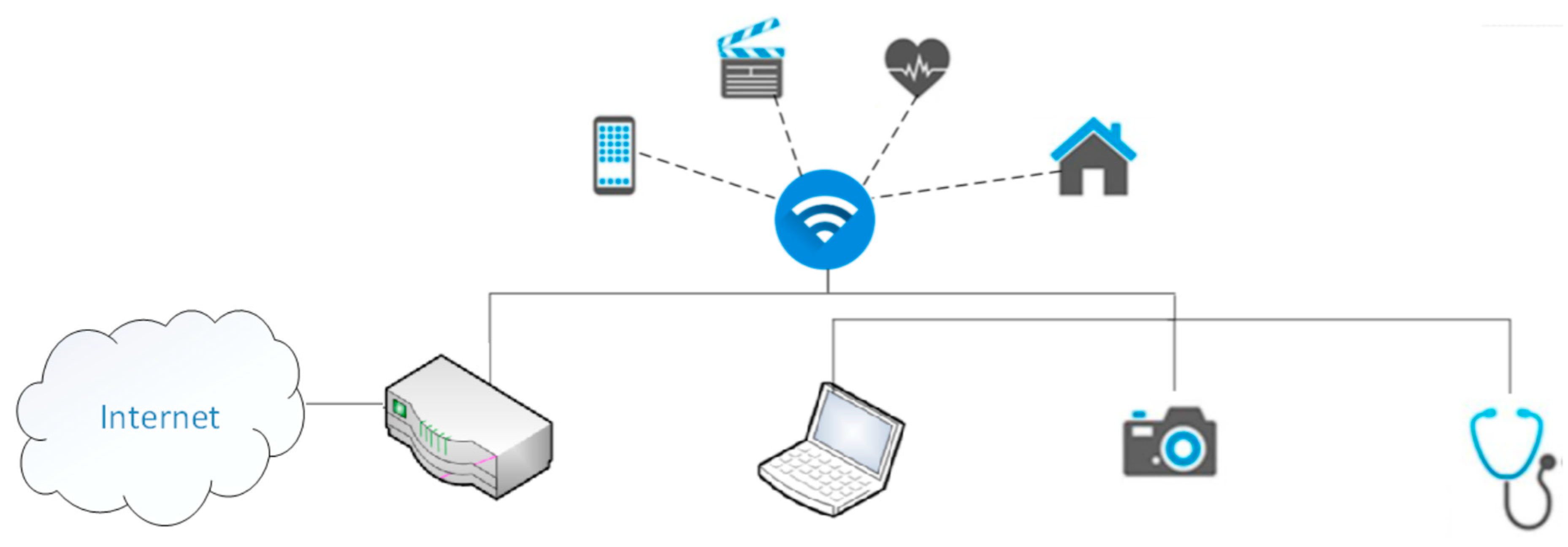
The research included an analysis of the processes of network traffic intensity in the LAN and IoT networks. The traffic was generated in a network consisting of three computers and a router. The router guaranteed access to the Internet for each computer or IoT device. The topology of the network is shown in Figure 1. One of the computers was equipped with Wireshark program for collecting packets in the local network and the Internet. The packets were collected within 1 hour for two cases: high network traffic (a web browser running with several web pages, applications using the Internet in the background, online computer games generating network traffic) and network traffic containing the low intensity of network packets.

R is a flexible (free) analytical environment with rich functionality that is used in much research and practical work on data analysis and knowledge discovery. Moreover, it provides embedded operations to facilitate the processing of tabular datasets; graphical data description mechanisms; rich libraries of analytical functions, including a wide range of statistical methods and knowledge discovery methods; and, most importantly, an interactive command interpreter and (for some platforms) a graphical user interface [29,30].

It is a language mainly used in bioinformatics. It enables conducting many types of statistical analyses such as modeling, tests, analysis of time series, and classifications. The main advantage of the R language is the possibility of creating its own packages and the possibility of implementing already prepared packages created by the users [31,32].

RStudio offers an integrated import of data, among others, from Excel files, which enables quick data analysis. It uses the readxl library to import spreadsheets. It is also possible to export data to Excel spreadsheet files using the xlsx library. For analysis, the collected network traffic with high packet density is divided into specific protocols. By dividing data into protocols, it is possible to create graphs or time series for each protocol and analyze them.

Protocols were separated from the total motion for detailed studies:

• ARP (address resolution protocol)—name recognition protocol;
• DNS (domain name system)—domain name protocol;
• SSDP (simple service discovery protocol)—detection protocol, devices;
• IGMP (internet group management protocol)—a multicast group management protocol;
• DHCP (dynamic host configuration protocol)—dynamic host configuration protocol;
• HTTP (hypertext transfer protocol)—www;
• TCP (transmission control protocol)—transmission control protocol;
• UDP (user datagram protocol)—user packet protocol.

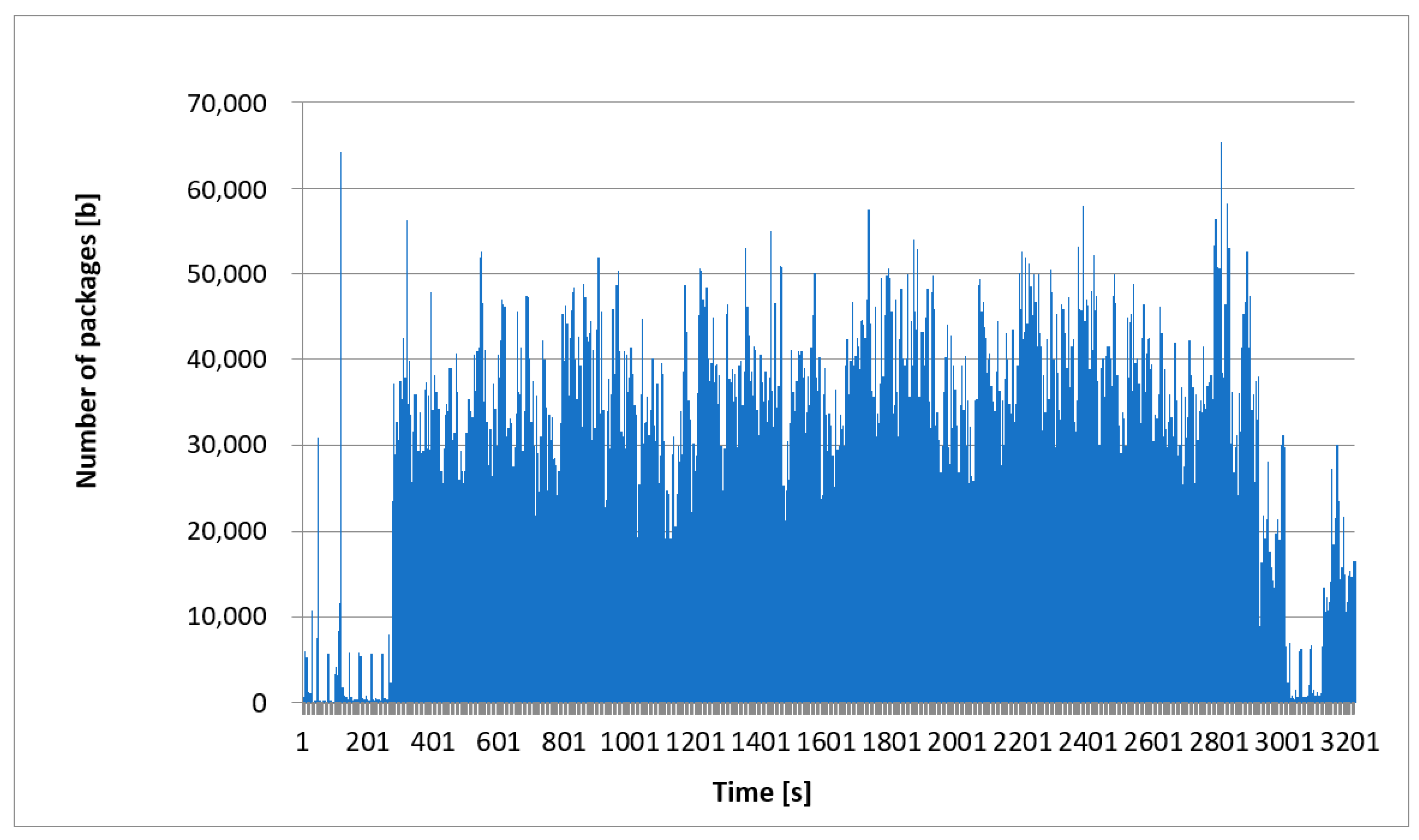
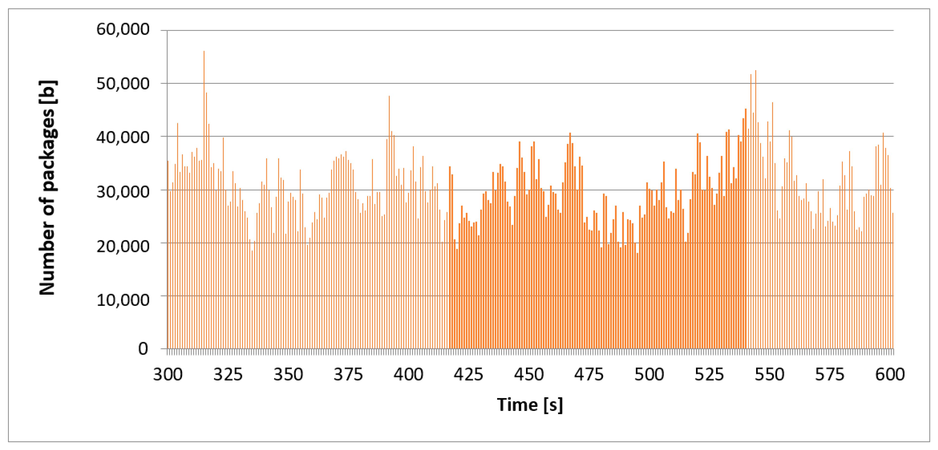
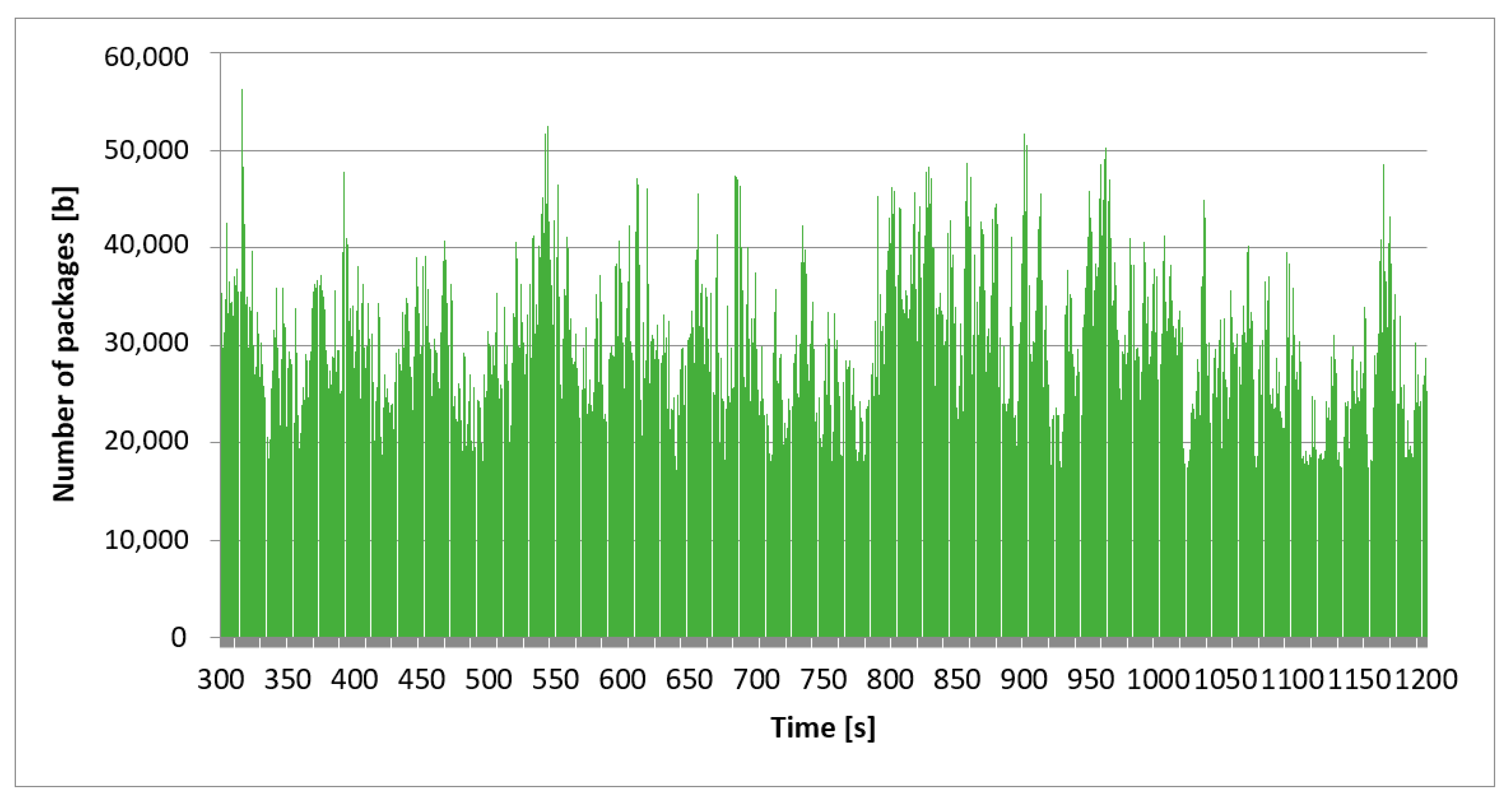
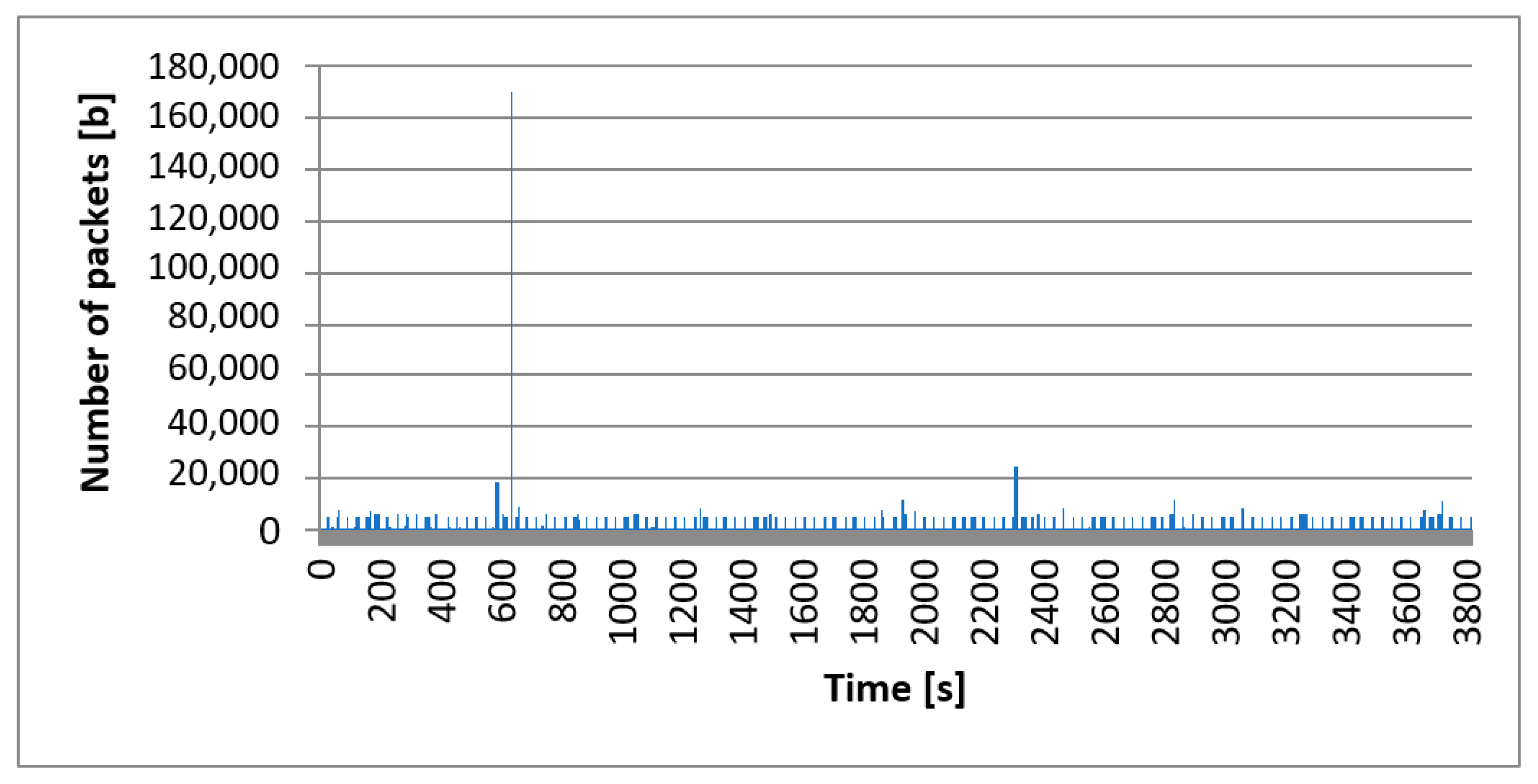
Most stochastic processes are characterized by the fact that these processes’ values are dependent on each other in time. Figure 2 shows the intensity of all network traffic analyzed. In this case, all protocols and the whole time scale were taken into account. The time range for high traffic was 3215 s. To confirm the stationary nature of the network traffic processes, we also show the collected traffic on different time scales. The diagram in Figure 3 presents the network traffic recorded in the time frame of 300 s, and Figure 4 in the time frame of 900 s. The diagrams present the same traffic but on different time scales. Our goal was to visually confirm that the graphs are similar in terms of self-similarity and “visually”, regardless of the time window. Despite the difference in the time scale between the charts, the individual processes’ nature remained unchanged and was similar. We can state that the autocorrelation coefficient was high. Due to the limited computing power, we analyzed a sample of 3215 s or almost 1 h. Such a value in the adopted analysis model allows for a reliable evaluation of the network “behavior”.

Despite the difference in time frames between the graphs, the character of individual processes remains unchanged, which confirms the thesis of stationarity and self-similarity. This study aimed to determine and evaluate the autocorrelation coefficient for various methods of determining the H-value (Hurst exponent).

In an R environment, we can determine the Hurst parameter H of a time series by linear regression of the $log\left(spectrum\right)$ versus $log\left(frequency\right)$ with frequency points accumulated into boxes of equal width on a logarithmic scale and spectrum values averaged over each box [30,33]. Robinson method estimates the Hurst coefficient in the frequency domain, by Robinson’s spectral density function (SDF) integration method. Given an estimate of the SDF for the input time series, this function estimates the Hurst coefficient of a time series by applying Robinson’s integral method (typically) to the SDF’s low-frequency end. A series with long-range dependence will show a spectral density with a lower law behavior in the frequency. Thus, we expect that a log–log plot of the periodogram versus frequency will display a straight line, and the slop can be computed as $1-2H$ [30,33,34]. In the standard method, one input puts an estimate of the spectral density function for the input time series. This function estimates the Hurst coefficient of the time series by performing a linear regression of $log\left(SDF\right)$ versus $log\left(frequency\right)$. A similar method is smoothed, but here frequencies are partitioned into blocks (the given argument controls the number of blocks) of equal width on a logarithmic scale, and the SDF is averaged over each block [30,33,34].

In this article, the following methods were chosen, and all worked directly with the sample values of the time series (not the spectrum) to estimate the Hurst parameter H of a long memory time series by one of several methods (Hurst coefficient estimation in the time domain). First, function aggvar, which is aggregated variance method, computes the Hurst exponent from an aggregated fractional Gaussian noise time series process variance. The original time series is divided into blocks of size $m$. Then, the sample variance within each block is computed. The slope $\beta =2H-2$ from the least square fit of the logarithm of the sample variances versus the logarithm of the block sizes provides an estimate for the Hurst exponent H [30,33].

The next function used is Higuchi method, which implements a very similar technique to the absolute value method. Instead of blocks, a sliding window is used to compute the aggregated series. The function involves calculating the length of a path and, in principle, finding its fractal Dimension $D$. The slope $D=2-H$ from the least square fit of the logarithm of the expected path lengths versus the logarithm of the block (window) sizes provides an estimate for the Hurst exponent H [33,34]. From the research, we can conclude that the Hurst coefficient estimated by these methods is very reliable.

5. Analysis of Network Processes for High-Intensity Traffic

The RStudio program performs statistical analysis for the overall traffic volume and determines the basic statistical parameters of the collected data, as shown in

Table 1. Statistical analysis for general network traffic.

Minimum	1st Quarter	Median	Average	3rd Quarter	Maximum
0	23,326	29,799	27,678	35,970	65,159

.

A detailed analysis of Hurst’s parameters was performed using the hurstexp command. There were used several methods, such as

-

Estimation of R/S;

-

Corrected R/S estimation by Hurst’s exponent;

-

Hurst empirical exponent;

-

Improved Hurst empirical exponent;

-

Hurst theoretical exponent.

This function is part of the pracma library, which contains a large number of functions for statistical, mathematical, and numerical analysis. The hurstexp command uses R/S (long-range) analysis to determine the Hurst factor. The results obtained are summarized in

Table 2. Hurst coefficient values for specific intervals (windows size).

Windows Size	2	4	8	16	32	64	128	256	512	1024	2048
R/S estmation	0.85	0.85	0.85	0.85	0.85	0.85	0.85	0.85	0.85	0.85	0.85
R/S improved estmation	0.99	0.99	0.99	0.99	0.99	0.99	0.99	0.99	0.99	0.99	0.99
Empirical exponent H	0.00	0.94	0.95	0.97	1.01	1.06	1.10	1.20	1.13	1.09	0.84
Improved empirical H	0.00	0.87	0.90	0.94	0.98	1.04	1.09	1.19	1.12	1.09	0.84
Theoretical exponent H	0.60	0.57	0.56	0.54	0.53	0.53	0.52	0.51	0.51	0.51	0.52

.

The resulting simulations show that regardless of the time window’s size, for the R/S estimation method, the value of the Hurst coefficient was constant. The empirical Hurst exponent changed. It increased to 1.2 for window 256 and then decreases to 0.84 for window 2048. Improved empirical Hurst exponent kept similar relations. It took lower values than the empirical Hurst exponent. The theoretical Hurst exponent reached the highest value of 0.6 for the smallest window and then decreased with the increase in the time window size. On the basis of the values of Hurst exponent, we carried out a study on the convergence of the results obtained by spectral regression [35]. Using the hurstSpec command, we determined the Hurst coefficient according to three methods. The hurstSpec command determines the time series’s Hurst coefficient by linear regression of the spectrum logarithm concerning the frequency logarithm. Frequency points are accumulated in equal width for the logarithmic scale. Spectrum values are averaged over each frame. The hurstSpec command uses the following methods:

-

Standard method estimates the Hurst exponent of the time series by performing a linear logarithmic regression of the spectral power density (SDF) in relation to the frequency’s logarithmic function.

-

Smoothed method is based on the standard method, but the only change is to divide the frequency into blocks of equal width, while the spectral power density (SDF) is averaged for each block.

-

Robinson method estimates the Hurst factor of a time series using Robinson’s integration method. This method uses low frequency to the end of a block of spectral power density (SDF) [1,29].

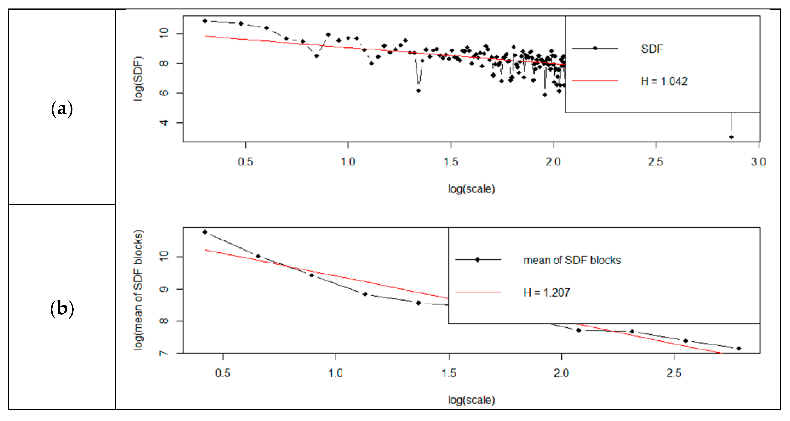
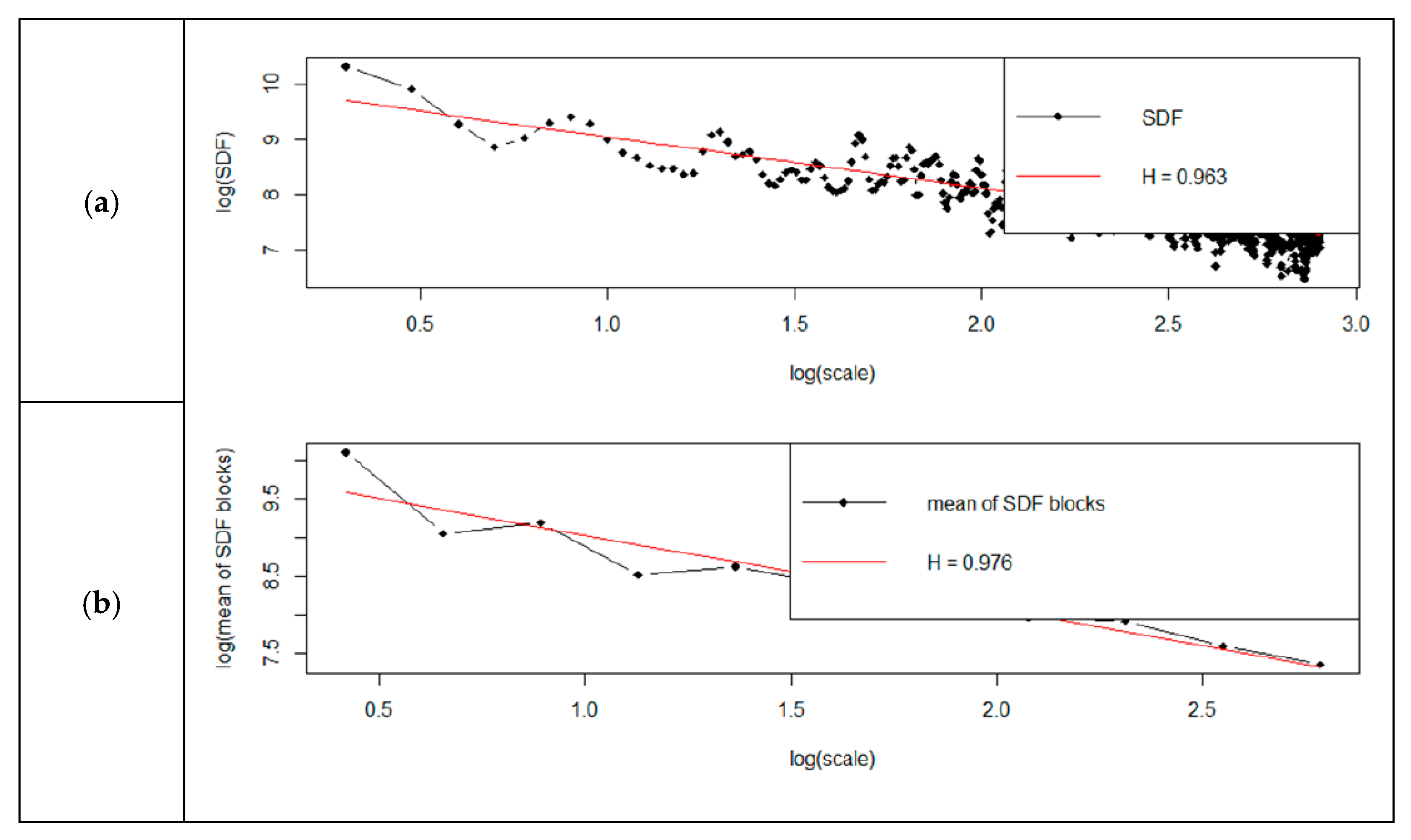
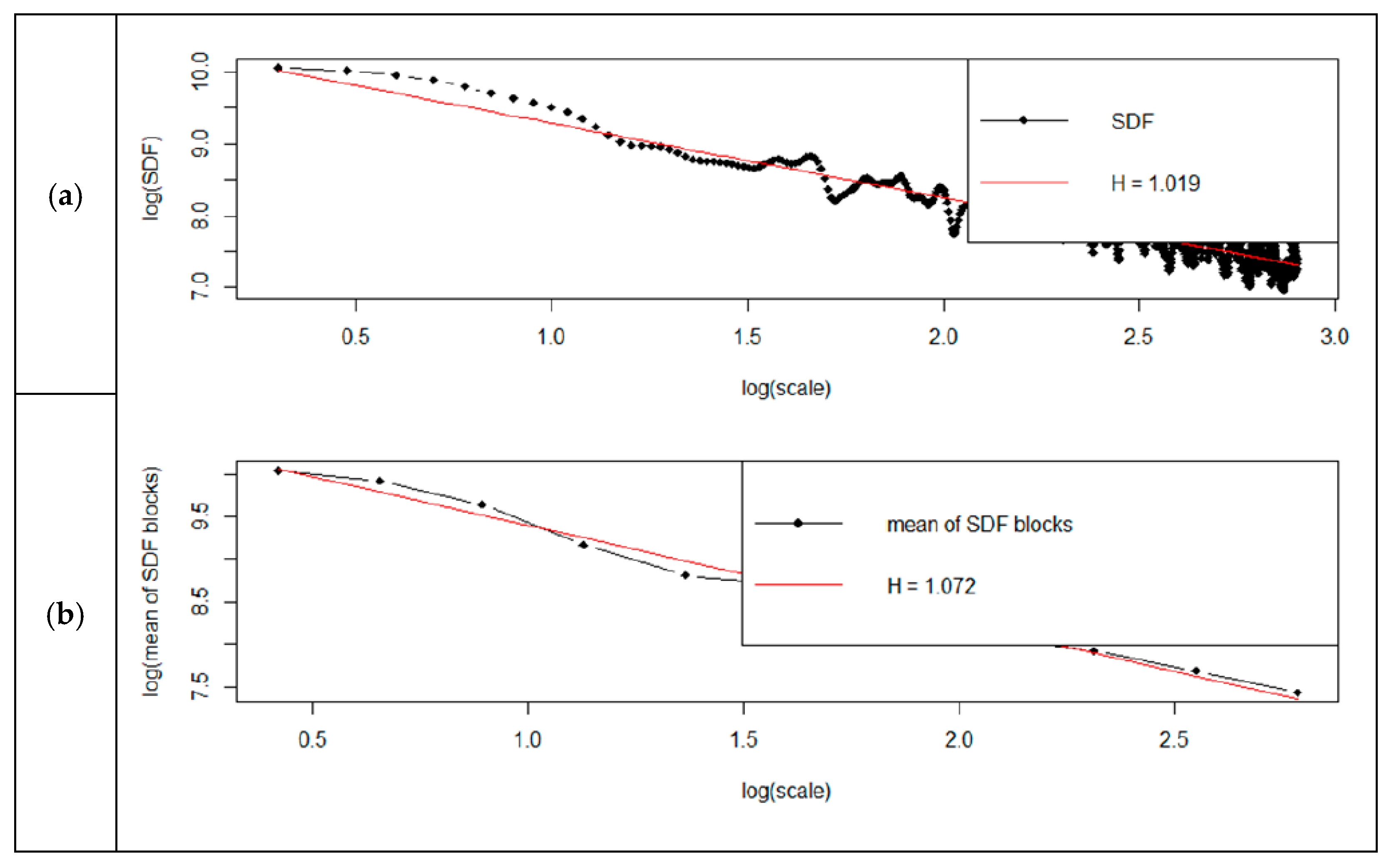
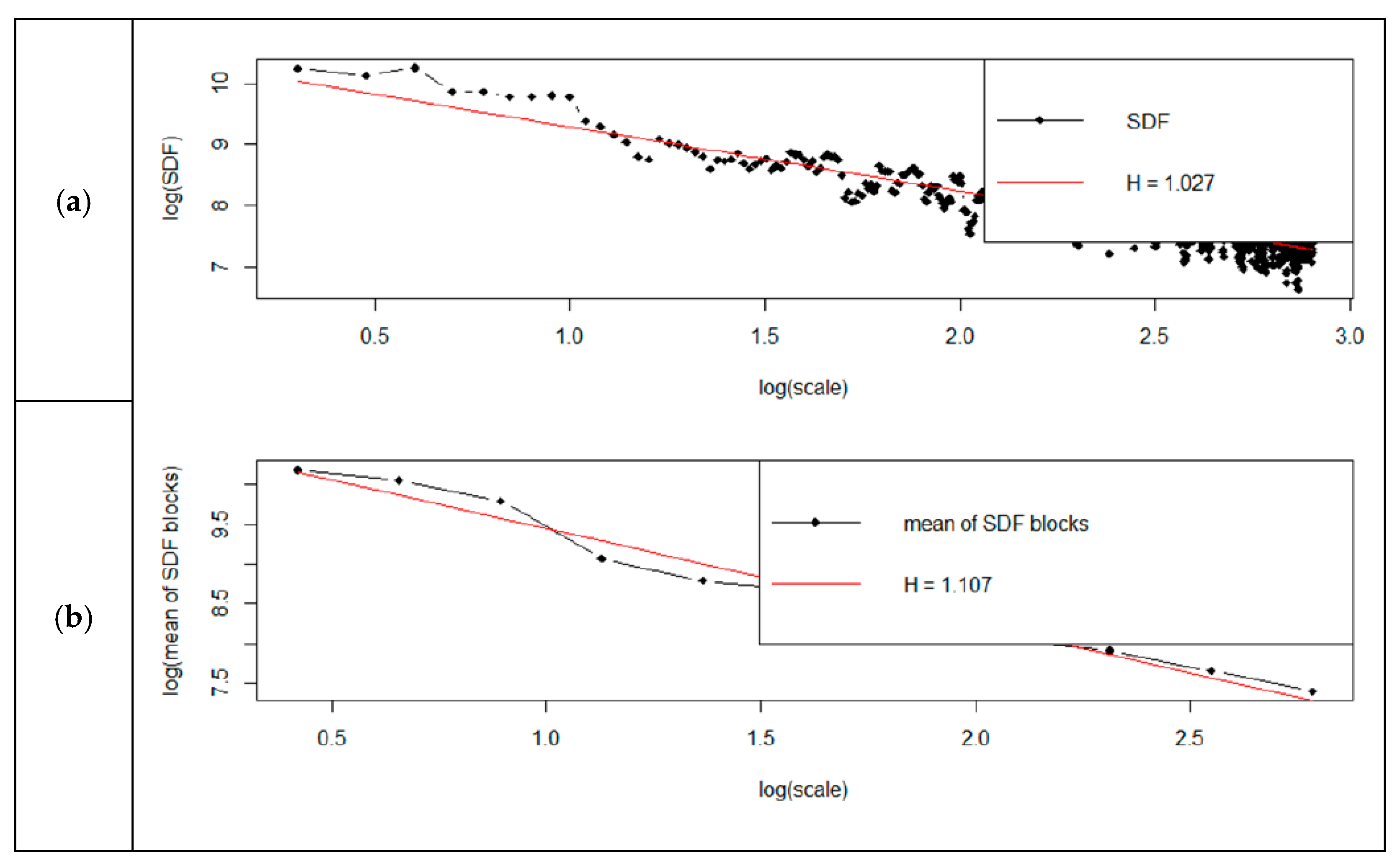
Evaluation of the Hurst coefficient by means of spectral regression showed that for the standard method, the H-value was 1.042; for the smoothed method, 1.207; and the Robinson method, 0.999. The discrepancy was therefore about 21%. The Robinson method returned a factor identical to that of the corrected R/S estimation. The hurstSpec command also offers the possibility to draw logarithmic graphs of spectral regression for standard and smooth methods. It is not possible to draw diagrams for the Robinson method. It is possible to draw diagrams according to four methods of spectral power density (SDF): direct, lag window, wax, multitaper [29,35].

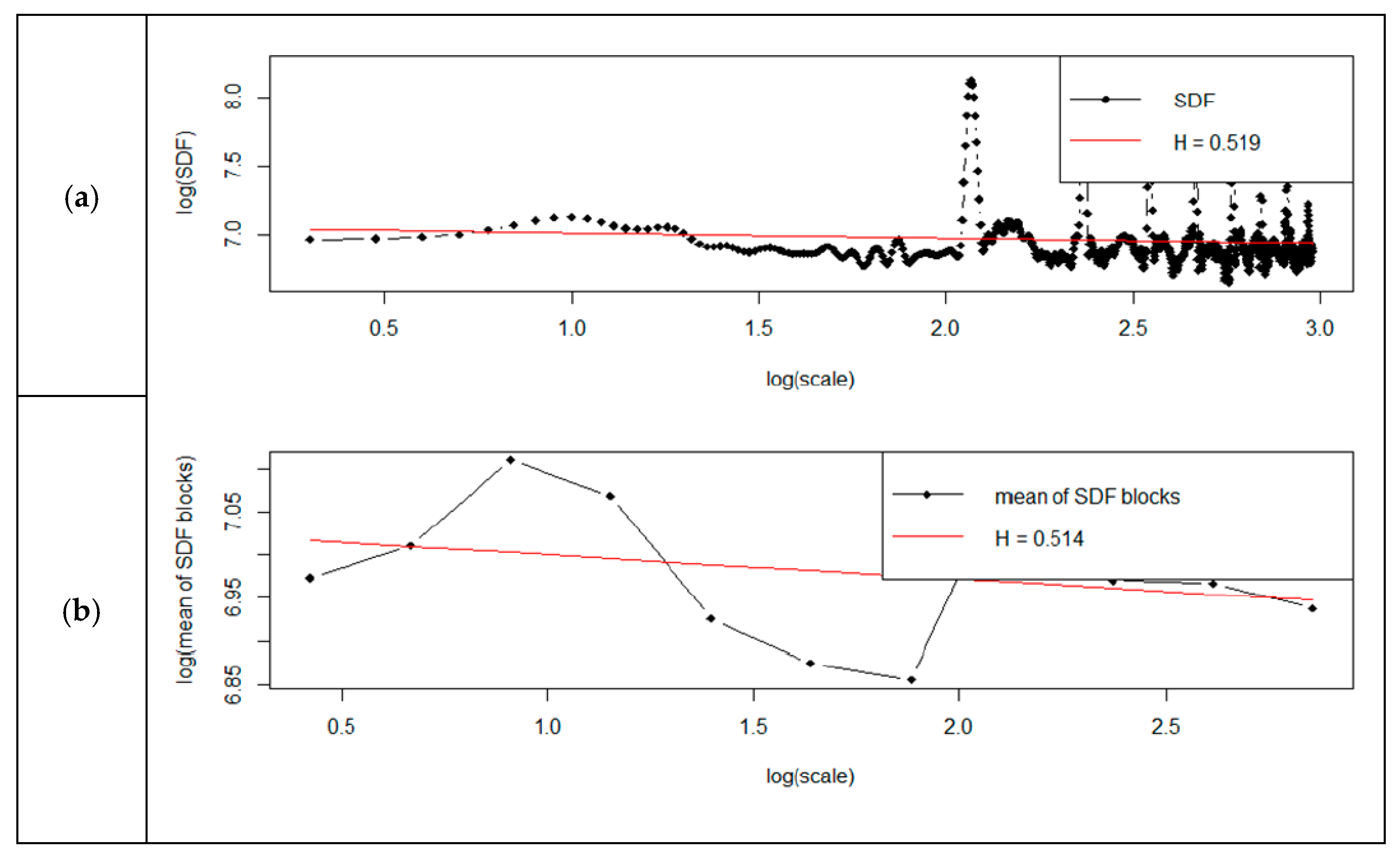
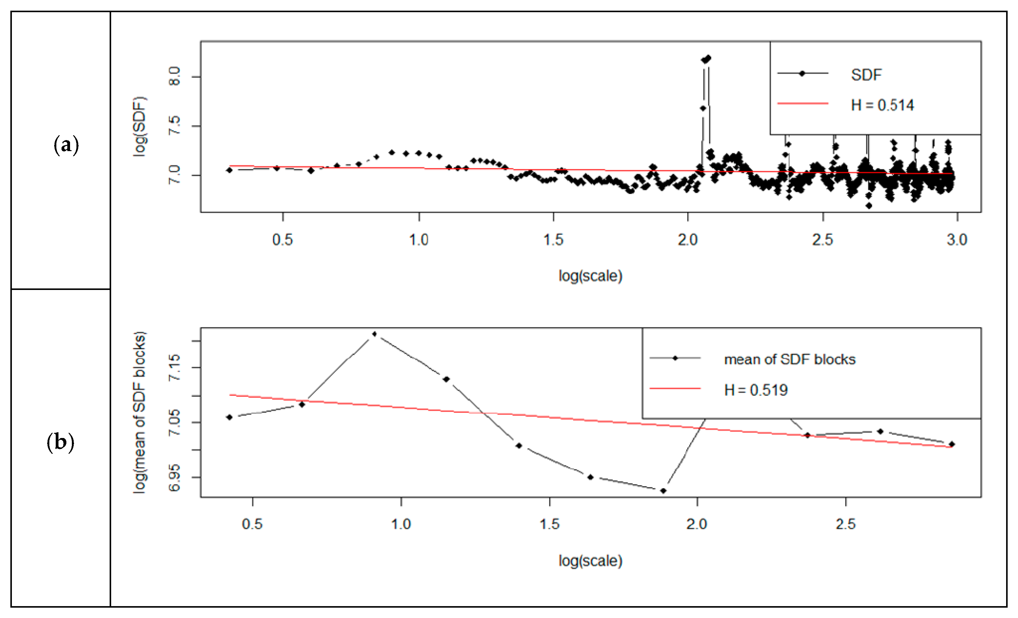
Detailed results of analyses are shown in Figure 5, Figure 6, Figure 7 and Figure 8. Each figure has two charts—(a) shows the standard method, (b) shows the smoothed method.

From the graphs (Figure 5, Figure 6, Figure 7 and Figure 8), it can be concluded that the determined Hurst factor depends on the chosen method of spectral power density (SDF). For the standard method, the Hurst factor is subject to a smaller scale of changes. It was between 0.96 and 1.04. For the smoothed method, the Hurst factor had a more significant variation, between 0.97 and 1.2.

The R language also offers other commands for determining the Hurst ratio. The RoverS command determines the Hurst factor by the scaled R/S range method. The data series are divided into several groups. The R/S statistics are determined, the number of groups is increased, and the calculations are repeated. The logarithmic graph R/S in relation to the number of groups is ideally linear, with a slope of H. The H-factor can be determined by using linear regression [2,21].

Table 3. Hurst coefficient values calculated by the RoverS method for a specific range.

Range	2	4	8	16	32	64	128
Value	0.80	0.81	0.82	0.82	0.81	0.85	0.89

below shows the Hurst exponent determined by the RoverS command.

The classic methods of determining the H-factor can generally be divided into two main domains. The first is the time domain, which contains the aggregated variance method, Higuchi’s [35] method, the rescaled range statistics method, and the detrended fluctuation analysis method. The second domain is the frequency domain by means of connections to Fourier or wavelet spectrum decay, for example, Lobato and Robinson [34], and includes the periodogram method, the modified periodogram method, and Whittle’s estimator [33].

The Hurst values determined by the RoverS command are close to the R/S estimation values calculated by the hurstexp command. It is not possible to calculate a factor value for a range higher than 128 because the values become collinear. The hurstBlock command estimates the Hurst factor in the time domain. It uses the following methods:

-

Aggvar—The series is divided into m groups. In each group, the variance is evaluated (against the average of the whole series). A measure of the variability of these statistics between groups is calculated. The number of m groups is increased and the process is repeated. Hurst exponent is determined by the linear regression of the slope of the ideal line graph.

-

Higuchi—In this case, it is assumed that the series has the character of noise, not motion. The series is divided into m groups. The total sum of the series is calculated to convert the series from noise to motion. Absolute differences in total sums between groups are analysed to estimate the fractal dimension of the pathway. The number of m groups is increased, and the process is repeated. The H-value is determined by the linear regression of a logarithmic chart [24,30].

The Hurst coefficient estimation showed that for the Aggvar method, the H value was 0.813, and for the Higuchi method it was 1.028. The discrepancy was therefore about 25%. The Hurst exponent values are determined by the hurstBlock command shapes within limits set by the other commands. It can be stated that the H-value estimated by these methods is reliable.

6. Analysis of Network Processes for Low Traffic

To ensure the correctness of the analysis, we also analyzed the case of low traffic. The time window was 3820 s. Similar tests were carried out for high traffic. The sample of motion is shown in Figure 9. It shows the volume of all network traffic, including all protocols in the full-time window.

As before, despite the difference in the time scale between the charts, the nature of individual processes remained similar. We can conclude that the autocorrelation coefficient is high, as well as for high traffic. It has been observed that traffic is repeated in time sequences. Statistical analysis was performed using the summary command. The results of the analysis are shown in

Table 4. Statistical analysis for general network traffic.

Minimum	1st Quarter	Median	Average	3rd Quarter	Maximum
0	0	167	777.3	294	169,962

.

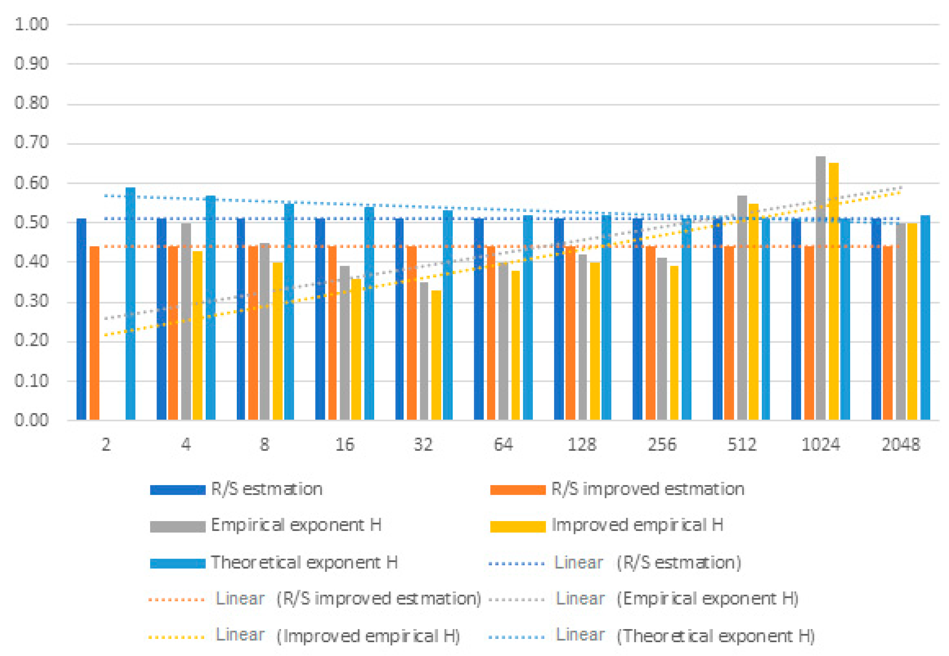
The Hurst exponent was determined for a given range. The detailed results are summarized in Figure 10. The Hurst exponent for estimation and improved R/S estimation did not change and assumes the values 0.51 and 0.44, respectively. The empirical exponent was 0 for interval 2. Its value ranged from 0.35 to 0.57. The improved empirical Hurst exponent had similar relationships. It assumed lower values than the empirical Hurst exponent. The theoretical Hurst exponent reached the highest value of 0.59 for the smallest range, after which it decreased as the range increased. The correctness of calculations was verified by determining the Hurst coefficient employing spectral regression.

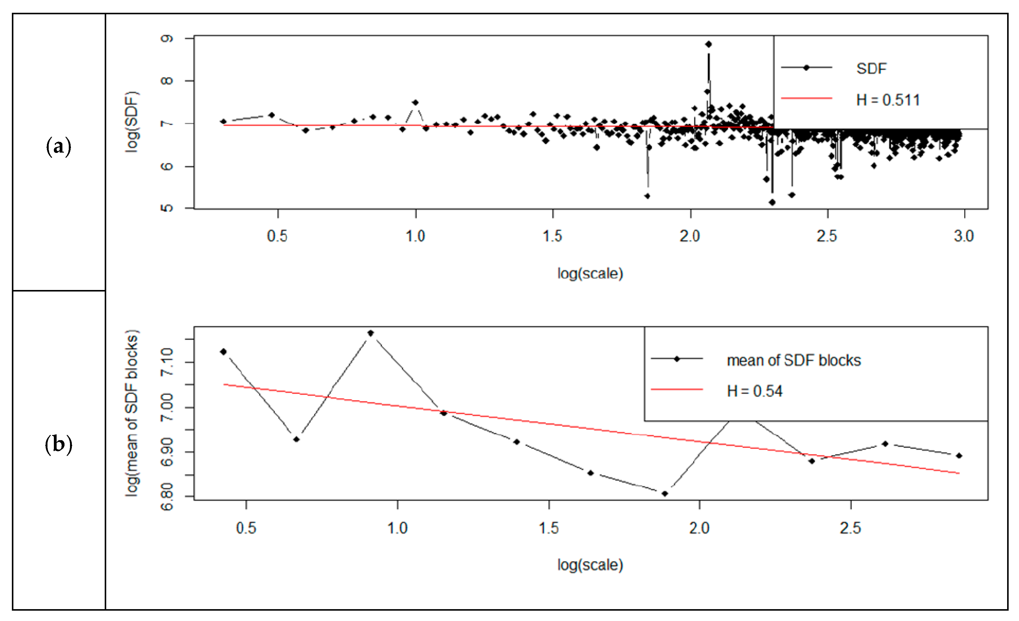
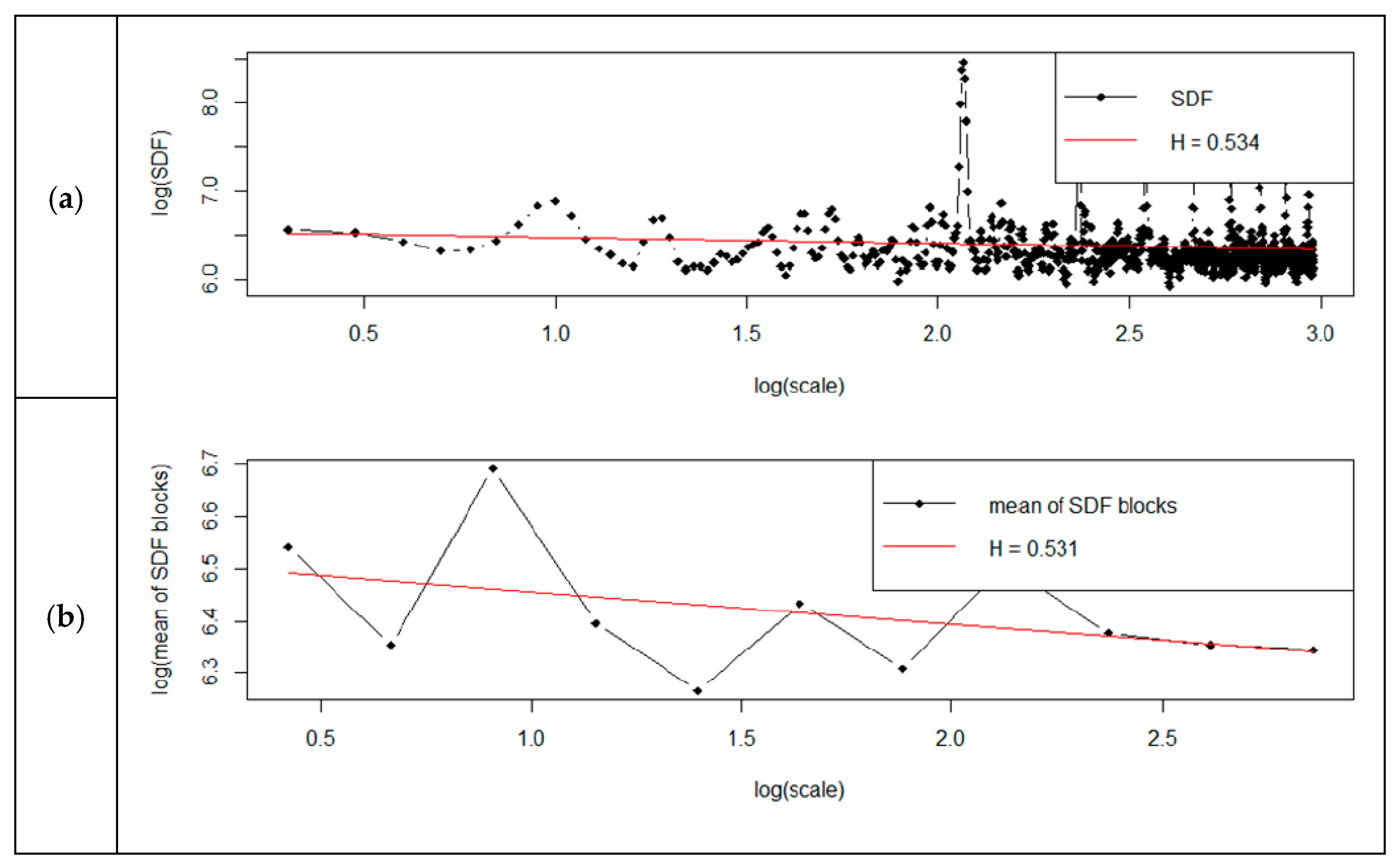
The Hurst coefficient obtained with the use of the hurstBlock method was within the ranges set by the other commands. We can conclude that the Hurst coefficient estimated by these methods was therefore reliable. The standard method returned a result identical to the R/S estimation. The Hurst coefficient evaluation using spectral regression showed that for the standard method, the H value was 0.51; for the smoothed method, it was 0.54; and for the Robinson method, it was 0.585. The discrepancy was, therefore, only 14%. Figure 11, Figure 12, Figure 13 and Figure 14 presents detailed charts presenting the standard method and the smoothed method chart.

Analysis of the obtained results shows that the determined Hurst exponent depended on the selected spectral power density (SDF) method. For the standard method, the Hurst exponent changed—it was between 0.51–0.54. The Hurst exponent had a similar scale of changes for the smoothed method and was between 0.51–0.53. Verification of the Hurst exponent using the RoverS command showed that the obtained results differed by up to 40%.

Table 5. H exponent values calculated using the RoverS method for a specific range.

Range	2	4	8	16	32	64	128
Value	0.70	0.66	0.64	0.52	0.27	0.34	0.47

shows the Hurst exponent values determined by the RoverS method.

Estimating the Hurst exponent using the HurstBlock method showed completely different results for the two methods. The Hurst coefficient estimation showed that for the Aggvar method, the H value was 0.485 and for the Higuchi method, the H value was 0.996. The discrepancy was therefore over 105%. The Hurst exponent determined by the hurstBlock command using the Aggvar method was within the other commands’ ranges. However, the Higuchi method’s estimated Hurst exponent was completely beyond the range of obtained Hurst exponent values determined by other methods.

7. Comparison of Results

The presented Hurst exponent calculations for network traffic processes with high and low packet intensity showed a significant discrepancy in the values obtained.

Table 6. Averaged values of Hurst exponent calculated for two types of network traffic.

Type of Network Traffic	High Traffic	Low Traffic
R/S estmation	0.85	0.51
R/S improved estmation	0.99	0.44
Empirical exponent H	1.03	0.46
Improved empirical H	1.00	0.44
Theoretical exponent H	0.54	0.54

presents the average Hurst exponent calculated by the hurstexp command for two general network traffic types. Therefore, the discrepancy for high-intensity traffic was 21% in extreme cases and only 13% in low-intensity.

It was found that high-traffic network traffic had a Hurst exponent close to 1, which underlines the self-similar nature of traffic. The results for the low-intensity variant confirmed the situation that the processes had the characteristics of the antipersistent movement, in which the Hurst exponent was in the range of 0 < H < 0.5. The process tended to return to the average ratio value. These values made frequent turns in the direction of movement.

Table 7. Hurst exponent values for two types of network traffic.

Type of Network Traffic	High Traffic	Low Traffic
Standard	1.04	0.51
Smooth	1.20	0.54
Robinson	1.00	0.58
Scaled R/S Range (RoverS)	0.83	0.51
Aggvar	0.81	0.48
Huguchu	1.03	0.99

shows the values determined using the hurstSpec, hurstBlock commands, and the average values of the RoverS command for tue two types of overall network traffic.

It was observed that for a process with high network traffic, the values calculated by different methods had a Hurst exponent similar to the value of 1. This confirmed that high-intensity traffic has strong properties of self-similarity and persistent traffic. According to the designated methods, the process with low network traffic had values close to the Hurst exponent of 0.5. This indicates that this process is random but also antipersistent, as shown by previously calculated exponents. The result calculated using the Higuchi method for a process of low intensity can be treated as an error because the result was not close to the value calculated by other methods. In the case of high intensity, the difference in results obtained reached up to 20%, which shows that not all algorithms can be used to assess the characteristics of traffic correctly. In the case of low traffic volumes and random character, the results cannot constitute a reliable assessment. A detailed analysis of selected protocols is presented in

Table 8. Average Hurst coefficients for selected protocols for two types of network traffic.

Protocol	ARP	DNS	SSDP	IGMP	DHCP	HTTP	TCP	UDP
High intensity of network traffic
R/S estmation	0.45	0.59	0.38	0.42	0.52	0.57	0.77	0.85
R/S improved estmation	0.41	0.70	0.32	0.15	0.27	0.76	0.88	0.99
Empirical exponent H	0.45	0.63	0.29	0.12	0.71	0.66	0.85	1.03
Improved empirical H	0.44	0.62	0.27	0.12	0.70	0.65	0.85	1.02
Theoretical exponent H	0.54
Low intensity of network traffic
R/S estmation	0.40	0.51	0.39	0.41	0.49	0.55	0.50	0.69
R/S improved estmation	0.34	0.53	0.32	0.13	0.28	0.72	0.48	0.72
Empirical exponent H	0.35	0.62	0.33	0.11	0.47	0.70	0.50	0.80
Improved empirical H	0.33	0.61	0.31	0.11	0.46	0.69	0.49	0.78
Theoretical exponent H	0.54

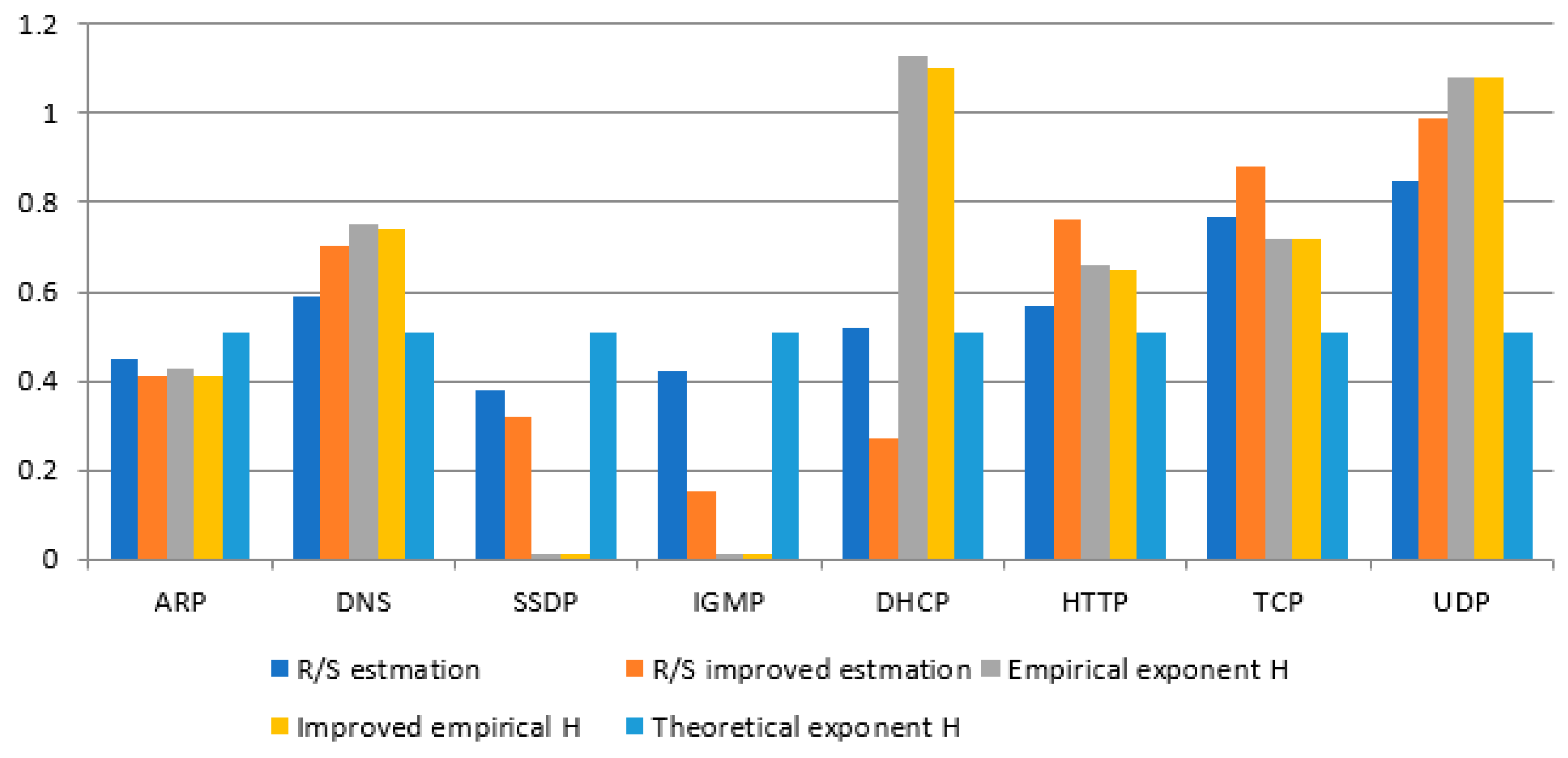
. Figure 15 shows a detailed comparison of the H-factor values for the time window size 1024. The results show that the Hurst values were dependent on the number of packets. The traffic was more stable, and the obtained signatures could be used to analyze traffic anomalies. Unfortunately, as the table and the graph show, the research found that these values were unbelievable, having a small number of packets, and cannot be used to build “real traffic behavior rules”. The results were averaged and aggregated according to protocols for two types of network traffic intensity.

It was found that the Hurst exponent for ARP, DNS, SSDP, and IGMP were similar for both types of network traffic intensity. For these protocols, the Hurst exponent for high traffic was higher by 5–15% than for low traffic. This was due to the number of packages and the measurement time. The values calculated by the R/S estimation method were similar. For improved R/S estimation, the Hurst exponent value increased for DNS in both types of traffic. Empirical values were also similar to different traffic volumes. The SSDP protocol increased the empirical Hurst exponent as opposed to high traffic. Hurst values for the ARP, SSDP, and IGMP had values in the range of 0–0.5, which indicated antipersistent traffic and a low level of self-similarity. The DNS protocol adopted Hurst exponent in the range of 0.5–1, which confirmed the nature of the persistent movement. DHCP had similar properties for R/S estimation and improved R/S estimation for both types of traffic. The Hurst exponent for the empirical method increased for high network traffic intensity, while for low traffic, the value decreased. The HTTP protocol had a similar Hurst exponent to the DNS protocol, which indicated that these protocols are closely related. They are necessary for correctly opening websites and web address translation. For both types of traffic, the Hurst coefficient values were in the range of 0.5–1. Hurst exponent for TCP and UDP depends on the number of packets. These protocols represent the largest number of packages in comparison with all other protocols. For high-intensity traffic, the Hurst exponent for the improved R/S estimation was higher than for standard R/S estimation. The values of the empirical and improved Hurst exponents were similar. The values were in the range of 0.5–1, and even for the empirical exponent, they went above the value of 1. For low traffic, the TCP protocol reached values close to 0.5, which indicates the randomness of the traffic. The UDP protocol assumed values in the range of 0.5–1 and value characteristics similar to the UDP protocol with high traffic. It has been observed that the values of the Hurst exponent of the method of improved R/S estimation were lower than the usual R/S estimation for most protocols. The values of the corrected empirical Hurst exponent were not much smaller than the empirical values. This was due to the method of the calculated exponent and also to the data itself.

8. Conclusions

Estimating the value of the Hurst exponent in the R environment showed that long-term relationships characterize network traffic. In the case of high traffic intensity, persistence was maintained, which emphasizes the general characteristics and nature of traffic generated on the examined nodes. Hurst exponent allowed us to analyze the current course, as well as predict future data behavior trends and what can be valuable in terms of security and detection of attacks or anomalies in the network. Thanks to the correct estimation of the Hurst exponent, creating appropriate patterns, we can prepare in advance for alarming situations and respond to a change in trend. Sudden deviations of the exponent value concerning the results obtained may probably be a sign of problems that for network traffic will indicate unusual network behavior potentially related to cybercriminal attack or network failure. Such network traffic analysis methods can be ideal for protecting critical data and maintaining the continuity of internet services offered.

Due to the threat of cyberterrorism, researchers are developing special systems to detect anomalies in network traffic. We can detect distributed denial of service (DDOS) attacks, which are extremely dangerous for systems, because these attacks can suspend the operation of certain services or servers. Therefore, it is extremely important in today’s world to analyze network traffic processes, allowing us to detect anomalies in the network and model the processes occurring in the network traffic.

The research allowed for the detailed determination of the Hurst parameter and the determination of the most accurate method, which coincides with analytical results. The nature of the traffic (its load) has an impact on the correctness of the analysis. The analyses showed that these methods could be successfully used for high traffic, but for low traffic, their reliability and use are random. The R package met expectations, allowing for the analysis and calculation of Hurst coefficients using various methods and functions. The selection of selected methods is crucial to determine the Hurst coefficient for specific protocols or general network traffic. Not all methods proved to be correct, but R software fully met the requirements previously set.

Research has shown that with a small number of packets, these values are unbelievable and cannot be used to build “real traffic rules”. The Hurst coefficient estimation showed that the discrepancy was over 105% for the low traffic method, which confirmed that low-intensity traffic analysis could not be taken as a reliable measure to predict network anomalies. In the case of high intensity, the difference in results obtained reaches up to 20%, which showed that not all algorithms can be used to assess the characteristics of traffic correctly.