Multi-Field Models of Fiber Reinforced Concrete for Structural Applications

Abstract

Short fiber reinforcement is added to concrete materials to improve a variety of performance measures related to structural safety, serviceability, and health diagnosis. Mesoscale models have been developed to understand the individual and collective actions of these fibers on various material properties. Those modeling efforts have predominately focussed on the mechanical (i.e., stiffness and strength) contributions of fibers. This paper introduces computationally efficient, semi-discrete representations of fibers within coupled mechanical and transport processes in cement-based matrices. Basic simulations are done to study: the use of conductive fibers for self-sensing; and the influences of fibers on early-age plastic settlement. It is found that the models can account for directional bias on fiber orientation, as may occur during material casting. With respect to plastic settlement, fibers may play competing roles: mechanical restraint offered by the fibers reduces settlement, whereas enhanced hydraulic conductivity along the fiber–matrix interface may increase settlement by facilitating the bleeding process.

1. Introduction

Short-fiber reinforcement is often added to concrete to improve its mechanical properties [1], particularly fracture toughness. Short fibers are also used to modify other aspects of concrete, including volumetric stability at early ages [2,3,4], resistance to spalling at high temperatures [5,6], bond properties of repair materials [7], structural composite behavior with steel reinforcement [8,9,10], and various electrical properties [11,12,13]. Along with the amount of fibers, the efficacy of fiber additions often depends on the distribution of fibers and characteristics of the fiber–matrix interface.

Effective medium theories have been developed to understand the global significance of fiber additions on the properties of interest (e.g., stiffness, strength, conductivity) [14]. The usefulness of such theories is limited, however, due to assumptions made regarding the distribution of fibers within the material volume. Numerical models have been developed to understand the individual and/or collective actions of these fibers on various performance measures. These modeling efforts have predominately focussed on the mechanical (i.e., stiffness and strength) contributions of fibers in both pre- and post-cracking conditions [15,16,17,18,19].

This paper introduces computationally efficient, semi-discrete representations of individual fibers within cement-based matrices that participate in electro-mechanical or hygro-mechanical phenomena. Voronoi Cell Lattice Models are used to represent the composite materials [20]. The fibers are discretized within the computational domain, such that the effects of fiber spatial distribution and orientation can be explicitly represented [21]. Basic simulations are conducted to study: the use of electrically conductive fibers for self-sensing; and the influences of fibers on early-age plastic settlement. The methods are verified through benchmark comparisons with numerical and theoretical models. It is found that the models can account for unintended directional bias on fiber orientation, as may occur during material casting. With respect to plastic settlement, fibers may play competing roles: mechanical restraint offered by the fibers reduces settlement, whereas enhanced hydraulic conductivity along the fiber–matrix interface may increase settlement by facilitating the bleeding process. Although the simulation efforts are limited to small component or unit-cell models, the low computational cost of the proposed approaches suggests future applications to structural concrete components.

2. Voronoi-Cell Lattice Model

Two related forms of lattice models are used to represent the variables associated with the multi-field phenomena considered herein. The mechanical behavior of the fiber-reinforced concrete is modeled using Rigid-Body Spring Networks, whose geometry is based on Voronoi/Delaunay tessellations of the nodal points. The potential field analyses utilize lattice models composed of conduit elements, based on the same connectivity defined by the Delaunay tessellation. In the present study, the collective approach is called the Voronoi-cell lattice model (VCLM) to emphasize the central role of the Voronoi diagram in establishing its desirable mechanical and potential flow qualities.

2.1. Mechanical Behavior

The mechanical behavior of the concrete is represented by a Rigid-Body-Spring Network (RBSN) [22,23,24], which is akin to other lattice models of concrete [25,26,27,28,29,30,31,32]. This section briefly describes its definition, with additional details given elsewhere [20].

Homogeneous regions of the material body are typically represented by randomly placed nodes, subject only to a minimum distance constraint. To construct material features within the domain, subsets of nodes are sequentially placed to define the vertices, edges, and faces of the desired features, prior to random filling of the feature volumes [33]. The RBSN is an assembly of rigid-body-spring elements. Each element is composed of a zero-size spring set, located at the centroid C of the corresponding Voronoi facet, connected to the nodes via rigid-arm constraints (Figure 1b). As mentioned above, element connectivity is determined by the Delaunay tessellation of the nodes; the dual Voronoi tessellation provides geometric measures that are used to determine element properties. With respect to the $n-s-t$ coordinate axes, defined local to Voronoi facet $ij$ (Figure 1b), the stiffnesses of the axial and rotational springs composing the spring set are

$$k_n=\beta k_s=\beta k_t=E\frac{A_{ij}}{h_{ij}}$$

(1)

$$k_{\varphi n}=E\frac{J_p}{h_{ij}}; k_{\varphi s}=E\frac{I_s}{h_{ij}}; k_{\varphi t}=E\frac{I_t}{h_{ij}}$$

(2)

where E is the elastic modulus of the material; $A_{ij}$ is the area of Voronoi facet; $h_{ij}$ is the distance between i and j; $I_s$ and $I_t$ are the second moments of the facet area about axes s and t, respectively; $J_p$ is the polar second moment of area of the facet; and $\beta$ is a factor related to macroscopic Poisson ratio $\nu$. Herein, $\beta =1$ renders the lattice elastically uniform, albeit with $\nu =0$ [34]. Complete representation of the Poisson effect, both macroscopically and in an element-local sense, has recently been accomplished using an iterative procedure [35].

The spring coefficients of Equations (1) and (2) form the diagonal of the material matrix

$$\mathbf{D}=(1-\omega )\mathrm{diag}\left[k_n,k_s,k_t,k_{\varphi n},k_{\varphi s},k_{\varphi t}\right]$$

(3)

where $0\le \omega \le 1$ is a scalar damage parameter used to model material fracture. Prior to fracture initiation, $\omega$ = 0. The element stiffness matrix (with respect to element local coordinates) is

$${\mathbf{K}}_{\mathbf{e}}={\mathbf{B}}^T\mathbf{D}\mathbf{B}$$

(4)

where $\mathbf{B}$ relates the spring generalized displacements to the nodal degrees of freedom of the element [22]

$$\mathbf{B}=\left[\begin{array}{cccc}-\mathbf{I}& {\mathbf{B}}_{\mathbf{12}}& \mathbf{I}& {\mathbf{B}}_{\mathbf{14}}\\ \mathbf{0}& -\mathbf{I}& \mathbf{0}& -\mathbf{I}\end{array}\right]$$

(5)

in which submatrices ${\mathbf{B}}_{\mathbf{12}}$ and ${\mathbf{B}}_{\mathbf{14}}$ are defined by

$${\mathbf{B}}_{\mathbf{12}}=\left[\begin{array}{ccc}0& -z_c& y_c\\ z_c& 0& -h/2\\ -y_c& h/2& 0\end{array}\right]; {\mathbf{B}}_{\mathbf{14}}=\left[\begin{array}{ccc}0& z_c& -y_c\\ -z_c& 0& -h/2\\ y_c& -h/2& 0\end{array}\right]$$

(6)

Recently, this elemental formation has been extended to accommodate large displacement analyses [36,37]. After transforming ${\mathbf{K}}_{\mathbf{e}}$ to global coordinates, the direct stiffness approach is used to assemble element stiffness matrices and internal force contributions into the structural equation set

$$\mathbf{K}\mathsf{\Delta }\mathbf{u}=\mathbf{R}+\mathbf{F}$$

(7)

in which $\mathsf{\Delta }\mathbf{u}$ is the increment in generalized nodal displacements; $\mathbf{K}$ is the system stiffness matrix assembled from the elemental components; $\mathbf{R}$ and $\mathbf{F}$ are the external and internal nodal force vectors, respectively. One advantage of this form of discrete model is in its ability to simulate tensile fracture with reduced mesh bias. In particular, implementations of the crack band model of Bažant et al. [38,39] within the rigid-body-spring model are objective with respect to mesh size and geometry [34]. Volumetric instabilities due to creep and thermal/hygral processes can be simulated by introducing rheological constructs and hygral/thermal units in the place of the axial springs of the rigid-body-spring elements [20]. Although volumetric instabilities and fracture are not considered in the simulations conducted herein, such modeling capabilities have been validated [18,34,40] and could be incorporated within extensions of this research.

2.2. Transport Behavior

Flow behavior is simulated using the same lattice topology, based on the Delaunay tessellation of the nodal points. The lattice elements serve as conduits of one-dimensional flow between the element nodes [20]. The cross-section area of a given conduit element is equal to the area of the Voronoi facet associated with the element nodes (Figure 1c). From a nodal point perspective, the lattice accurately simulates uniform flow through homogeneous materials subjected to a potential difference (i.e., the random lattice design does not affect the condition of uniform flow). The lattice model accommodates both steady-state and transient solutions. In cases where crack-assisted flow is of interest, a dual lattice approach is effective [41,42,43,44]. The field of displacements (for mechanical behavior) is represented at the Voronoi generator points, whereas the potential field is represented at the Voronoi vertices. Cracking is not considered in this study, so a conventional approach (where the mechanical and flow network nodes are coincident with the Voronoi generator points [20]) is employed.

The case of moisture diffusion, which is used to describe the modeling approach, is analogous to the cases of electrical and hydraulic conductivity considered later. Established approaches are used for modeling moisture diffusion in cement composites, the convective boundary conditions at exposed surfaces, and the coupling of the diffusion and strain analyses [45]. For isothermal conditions, with no sinks or sources present, the governing equation for transient diffusion problems is

$$\frac{\partial h}{\partial t}=\mathrm{div}\left[D\left(h\right)\mathrm{grad}h\right]$$

(8)

where h is the pore relative humidity and D is a humidity dependent diffusion coefficient, which is a scalar quantity for isotropic conditions. The problems considered hereafter do not involve the dependence of D on the field quantity. The semi-discrete form of Equation (8) is

$$\mathbf{M}\dot{\mathbf{H}}+\mathbf{K}\mathbf{H}=\mathbf{f}$$

(9)

where $\mathbf{H}$ is the vector of nodal relative humidities and the dot over $\mathbf{H}$ indicates time derivative. The system matrices, $\mathbf{M}$ and $\mathbf{K}$, are assembled from the elemental capacity and diffusivity matrices, respectively:

$${\mathbf{M}}_{\mathbf{e}}=\frac{h_{ij}{A}_{ij}}{6d}\left[\begin{array}{cc}2& 1\\ 1& 2\end{array}\right],$$

(10)

$${\mathbf{K}}_{\mathbf{e}}=D\frac{A_{ij}}{h_{ij}}\left[\begin{array}{cc}\hfill 1& \hfill -1\\ \hfill -1& \hfill 1\end{array}\right]$$

(11)

as would be done for the finite element analysis of potential flow problems using two-node elements [46]. In the elemental capacity matrix, d = 1.0, 2.0, and 3.0 for 1D, 2D, and 3D networks, respectively. The ensuing discussions pertain to electrical or hydraulic conductivity, rather than diffusivity, but the equations representing potential flow take the same general form.

3. Models of Fiber Reinforcement

Much effort has been devoted to modeling the strength and stiffness contributions of fibers to the behavior of hardened concrete. There has been interest in explicitly representing individual fibers, such that their local and collective effects can be simulated [21,47,48,49,50,51,52]. Such models permit the study of fiber distribution non-uniformity and its influence on the desired properties of the composite material, including cracking behavior during strain hardening [18,53].

A prime consideration is the balance between computational efficiency and accuracy in representing each fiber. On one end of the spectrum, fibers can be modeled using volume elements. This allows for accurate representation of the elasticity of the fiber and the possibility for directly modeling the fiber–matrix interface. Interface features (e.g., the lugs on ordinary steel reinforcing bars) can be explicitly represented [54,55]. This approach is computationally expensive, however, which limits the number of fibers that can be considered.

The number of computational degrees of freedom can be drastically reduced by modeling fibers as series of simple structural elements (e.g., line elements such as truss or frame elements). These line elements interact with the matrix via bond-link elements that account for relevant behaviors of the fiber–matrix interface [23,56]. Going a step further, by constraining the actions of the fibers to the kinematics of a particle network representing the cement-based matrix, fiber additions do not inflate the number of computational degrees of freedom [21]. The research presented herein employs this semi-discrete approach, which enables the inclusion of larger numbers of fibers. To have benchmark results for comparison, volumetric representations of individual fibers are also considered. For both approaches, emphasis is placed on modeling the individual and collective effects of fibers on transport processes, which has received scarce attention within the cement-based composites community.

The positioning of the fibers needs to be specified. Fiber locations can be based on sectional analyses [57,58,59] or 3D imaging [17,60,61,62], which have the advantage of capturing directional and concentration biases caused by the casting process. Alternatively, as done herein, a procedure is used to sequentially place fibers in the computational domain without positional or directional bias. The spatial coordinates of the centroid of a trial fiber are assigned using a uniform random number generator. The orientation angles of the fiber are then determined using the algorithm of Knop [63]. To avoid fiber intersections, a minimum allowable distance is maintained between fibers [64]. Trial fibers that meet the minimum distance constraint are retained within the material volume. For the unit cell simulations of transport phenomena presented hereafter, periodic boundary conditions are implemented for fibers intersecting the domain boundaries.

3.1. Volumetric Representation of Fibers

The material is modeled as a two-phase composite consisting of short-fiber inclusions embedded within a homogeneous matrix. The cross-section and length of fibers form part of the continuum, as shown in Figure 2. Individual fibers are discretized by placing nodal points within the domain using regular patterns. Herein, cylindrical fibers are approximately modeled (Figure 2b), but other cross-section shapes are also possible. The matrix phase, which forms the remainder of the material volume, is then populated with randomly placed nodes. The lattice model formed from this nodal point set accommodates analyses of both the scalar field(s) associated with potential flow and the vector field of displacements associated with mechanical behavior.

For the potential flow analyses, periodic boundary conditions are realized by: (1) positioning fibers irrespective of the domain boundaries; (2) placing any external portion of the fiber on the opposite side of the domain; and (3) introducing a special conductivity element that connects the nodes on the opposing faces, such that continuity of flow is maintained over the fiber length. This is shown in Figure 2c for the two-dimensional case. In Figure 2, the lighter colored fibers intersect one of the faces of the unit cell, whereas the darker colored fibers reside fully within the unit cell. The same discretization scheme is used for simulating mechanical behavior, but without the mechanical connection between corresponding nodes on opposing faces.

3.2. Semi-Discrete Representation of Fibers

In contrast to the volumetric representation of fibers described above, fibers can be freely positioned within the computational domain, independent of the background mesh representing the matrix material. A fiber element is produced wherever the fiber intersects a Voronoi facet, as shown in Figure 3. The fiber element introduces stiffness and/or conductivity, as the case may be, between nodes i and j associated with the Voronoi facet. In this way, the addition of fibers does not increase the number of computational degrees of freedom. For the illustrative examples presented in Section 4 and Section 5, the fibers are placed uniformly at random within the composite material domain. Other arrangements of fibers are possible, such as those resulting from casting [61] or extrusion processes. The semi-discrete fiber models are generally applicable to different fiber types, in the sense that the program routines utilize fundamental properties of the fibers (e.g., length, diameter, stiffness and/or conductivity of the fibers.) For cases where slippage occurs along the fiber–matrix interface, bond properties must also be specified.

3.2.1. Mechanical Behavior

An axial spring is inserted at each point of intersection of a fiber with a Voronoi facet [21]. The spring is aligned with the fiber direction. The force–displacement actions of the spring are related to the local ($i-j$) nodal degrees of freedom through rigid-arm constraints, similar to those of the rigid-body-spring network. Prior to matrix fracture, the fibers are assumed perfectly bonded with the matrix. The axial stiffness of the spring associated with each fiber element is determined using shear-lag theory [65]. In this way, stress transfer between the matrix and fibers appropriately depends on fiber aspect ratio and modular ratio.

This semi-discrete approach can simulate the debonding and pullout of fibers that bridge matrix cracks [21], based on the micro-mechanical model of Naaman et al. [66]. During the debonding/pullout processes, load is transferred between the material phases along the embedded lengths of the fibers, independently of mesh size [18,67]. For the illustrative examples considered herein, however, slippage along the matrix–fiber interface is not considered. The fibers are assumed to be fully bonded to the surrounding matrix material.

3.2.2. Transport Behavior

Akin to the approach for modeling the stiffness contributions of fibers, fibers contribute to the diffusivity (or conductivity) of the composite material wherever they intersect a Voronoi facet (Figure 3). The elemental form of the diffusivity contribution between nodes i and j is similar to that of Equation (11)

$${\mathbf{K}}_{\mathbf{f}}=D_f\frac{A_f}{h_f}\left[\begin{array}{cc}\hfill 1& \hfill -1\\ \hfill -1& \hfill 1\end{array}\right]$$

(12)

where $A_f$ is the cross-sectional area of the fiber; $D_f$ is the diffusivity of the fiber material in its axial direction; and $h_f$ is the projected length of $h_{ij}$ in the direction of the fiber. For the planar illustration of the lattice network shown in Figure 3, $h_f=h_{ij}cos\theta$. In this way, the total length of the fiber is preserved when crossing multiple Voronoi facets

$$l_f\approx \sum _{k=1}^N{h}_f^k$$

(13)

where N is the number of facets crossed by the fiber. In Equation (13), strict equality is achieved if the fiber end conditions are considered.

3.2.3. Transport Behavior: Model Verification

The discrete (volumetric) approach and proposed semi-discrete approach are compared for the case of a fiber(s) embedded in a plate of homogeneous material. Domain discretization for the discrete approach is shown by the Voronoi diagram in Figure 4a. A similar diagram is used for the semi-discrete approach, but without the structured arrangement of cells representing the fiber. For both cases, the fiber is centrally positioned and aligned with the direction of flow, which is induced by a potential difference $\mathsf{\Delta }\varphi$ = 1 acting across the model domain. The top and bottom surfaces act as perfect insulators. For the purposes of illustration, the fiber has aspect ratio $l_f/d_f$ = 50 and conductivity ratio ${\sigma }_f/{\sigma }_m$ = 1000. By comparing potential values along the plane of symmetry (Figure 4b,c), close agreement between the model results is evident. The semi-discrete approach is versatile in that fibers of different length, orientation, etc., can be placed in the domain without modification of the background mesh representing the matrix phase, as shown by the results in Figure 4d. Notably, the random lattice discretization of the matrix phase of the material does not produce artifacts in the contour plots. This lack of artificial heterogeneity in the background lattice allows for more precise descriptions of the fiber contributions to composite behavior.

4. Electro-Mechanical Analyses with Applications to Self-Sensing

4.1. Background

With respect to the electrical properties of fiber concrete, conductivity (or resistivity) of the composite material is commonly of interest. Changes in composite resistance due to applied loading can be measured and used for self-sensing of structural concrete [12]. Variations in voltage along the periphery of fibrous sensing skins have been used to produce conductivity maps and characterize damage within the enclosed region of interest [68]. Such self-sensing capabilities are potentially useful for the condition assessment of structural concrete.

Three behavioral regimes have been used to characterize composite conductivity. At low fiber contents, the fibers are electrically isolated from one another within the lowly conductive cement-based matrix. In this condition, conductivity of the composite increases with increasing fiber content, but at a relatively low rate. Effective medium theories have been developed to describe the dependence of composite conductivity on the amount, aspect ratio, conductivity, and orientation distribution of the fibers [14]. By increasing the amount of fibers, the number of direct contacts (or near contacts) between fibers also increases. Within the second regime, dramatic improvements in composite conductivity result from the establishment of those longer conductive pathways and, ultimately, percolation clusters across the region of interest [11,12]. In the third regime, composite conductivity continues to increase with increasing fiber content, but at a lower rate after achieving a sufficient degree of percolation. The simulations presented herein mainly involve the first behavioral regime, due to the relatively low fiber dosages and low aspect ratios considered.

4.2. Solution Scheme

The electro-mechanical coupling is established using a staggered solution scheme. The base resistance of the numerical specimen is calculated for the case of no applied loading. Loading is then applied incrementally. For each load increment, the nodal positions are determined. The associated element strains are then used to calculate updated values of composite resistance. For the examples considered herein, planar arrays of nodes are placed along the negative and positive x-faces of the 3D domain (Figure 5). These nodes serve as electrode surfaces or grids for imposing a potential difference in the x-direction. The planar positioning of the nodes also facilitates the calculation of electrical current between the opposing faces.

Fibers are placed uniformly at random within the cell. At this stage of model development, lower fiber contents are analyzed and therefore fiber-to-fiber contact is not a consideration. The aspect ratio of the fibers is $l_f/d_f$ = 50, where $l_f$ is 0.5L. The conductivity ratio is set at ${\sigma }_f/{\sigma }_m$ = 1000. Whereas this ratio is much smaller than that between conductive fibers and concrete, which can be on the order of ${10}^8$ [13], it is sufficient for examining basic operations of the model. For the discrete (volumetric) modeling of fibers, the fibers are discretized as indicated in Figure 2b. For both the discrete and semi-discrete models, random filling of the matrix volume with nodal points employed a minimum distance constraint of $L/33$.

The influence of conductive fibers on potential flow is illustrated in Figure 6, which is based on earlier simulations with lesser amounts of fibers. Flow initiating on the left side of the figure moves within and between the conductive fibers. The color coding of the streamlines is not a quantitative indicator but was done to distinguish the different flow paths.

4.3. Verification of Conductivity Simulations

As primary conditions for simulating electrical behavior of fiber-reinforced composites, the model should account for the amount, aspect ratio, and orientation of the fibers, as well as the differing conductivities of the fiber and matrix materials. Effective medium theories have been useful in estimating fiber composite properties (including conductivity) when basic requirements are met regarding the orientation distribution of the fibers. In this study, the equivalent inclusion method (EIM) of Hatta and Taya [14] provides benchmark values for verifying the lattice models. Whereas the EIM was developed for heat conduction problems, it is analogous to Eshelby’s equivalent inclusion method in elasticity [69]. The EIM applies to potential flow problems, in general, including the electric conductivity simulations presented herein. The expression for determining composite conductivity is given in Appendix A. For the assumed model parameters, Figure 7 compares estimates of composite conductivity according to the EIM of Hatta and Taya with bounds of the Hashin–Shtrikman solution [70].

To verify the lattice models, a potential difference $\mathsf{\Delta }\varphi$ = 1 is applied across the unit cell shown in Figure 5. As previously mentioned, the potential is assigned to nodal arrays along each surface normal to the x-direction, separated by distance $L_e$, according to $\varphi \left(x\right)=\mathsf{\Delta }\varphi x/L$. Fibers were not placed close to the boundaries, which facilitated domain discretization and the assignment of nodal potentials. The influence of this condition on the conductivity simulations, which appears to be secondary, was modeled using parallel and series constructions of the regions with and without fibers [71]. Conductivity of the composite material, $\sigma$, was determined using

$$J=-\sigma \frac{\varphi \left(L\right)-\varphi \left(0\right)}{L}$$

(14)

where J is the average current density and $\varphi \left(L\right)-\varphi \left(0\right)$ is the potential difference between the faces of the unit cell. Average current density was found by summing nodal flux values over either of the x-faces, and dividing by the face area. The procedure for calculating nodal flux values is outlined in [20].

Results of the discrete (volume element) approach to modeling fibers are compared with the EIM values in Figure 8, for small volume fractions of fibers up to $V_f$ = 0.01. The limitation on fiber dosage is due, in part, to the computational expense of models with larger volume fractions. For higher fiber contents, contact between fibers is difficult to avoid, along with the eventual formation of percolation clusters. Seven numerical specimens, differing only in their random distributions of fibers, were produced for each fiber volume fraction considered.

Several observations can be made regarding the conductivity values plotted in Figure 8. The lattice model results exhibit the expected trend: conductivity of the composite material increases as the dosage of conductive fibers increases. The mean values given by the lattice model agree well with those of the EIM of Hatta and Taya. In a separate study, experimental measurements of AC composite conductivity of steel-fiber reinforced cementitious materials agreed well with the EIM, when some degree of preferential alignment of the fibers was considered [13].

The simulated conductivity values exhibit scatter about the respective mean values. The error bars in Figure 8a indicate one standard deviation from the mean value. In Figure 8b, the simulated conductivity values have been normalized by the corresponding EIM values, ${\sigma }_{EIM}$, such that the entire set of results can be plotted together. These results indicate that there is correlation between the degree of fiber alignment in the x-direction and the conductivity values. The degree of alignment is expressed by the average of $cos\alpha$, where $\alpha$ is the angle between each fiber axis and the x-direction. As expected, preferential alignment produces higher conductivity values. The differing random realizations of the fiber–matrix pathways for conductive flow may also contribute to the scatter in the conductivity values. The model capabilities are potentially useful in understanding the effects of alignment bias due to the production/casting processes and container boundaries. Non-uniform or poorly aligned fiber distributions may strongly influence the fracture properties of fiber-reinforced concrete [57,60,61,72]. The severity of alignment bias on composite conductivity has not been examined herein, since all fibers distributions are, in a nominal sense, uniformly at random.

The same set of parameters is used for simulating composite conductivity using the proposed semi-discrete modeling approach. Regardless of the fiber dosage, the number of computational nodes representing the composite material, $n_c$, does not change and is equal to $n_b$ (≈16,000), which is the number of nodes defining the background lattice representing the matrix material. This is in contrast to the discrete approach for which computational cost grows with fiber dosage, as shown in Figure 9. For perspective, nodal counts for a case of a higher fiber aspect ratio are included in the figure. It is apparent that the full volumetric discretization of the fibers becomes cost prohibitive as the volume fraction or aspect ratio of the fibers increases. In other words, the proposed semi-discrete approach has a clear advantage with respect to its lower computational complexity. For the parameter set and maximum fiber dosages considered herein, $n_c/n_b$ = 7.8, which is nearly an order of magnitude difference in the number of nodes.

As seen in Figure 10, similarly good agreement with the EIM curve is observed for lower $V_f$ values, but the model results tend to drift upward as $V_f$ grows. At lower $V_f$ values, the background mesh is sufficiently fine such that the fibers are electrically isolated from one another. In other words, fiber elemental contributions to diffusivity (as per Equation (12)) are introduced to different matrix nodes, such that any two fibers are effectively separated by matrix material. The discrete approach satisfies this condition by design of the fiber cross-section, as shown in Figure 2b. The semi-discrete fibers could remain electrically isolated for much larger $V_f$ provided the density of nodes representing the matrix was increased accordingly. However, the computational efficiency advantages of the semi-discrete approach would then be lessened. Nonetheless, these simulations verify accuracy of the semi-discrete approach for modeling the transport behavior of fibers. Notably, the semi-discrete approach also captures the influence of directional bias of the fibers on composite conductivity, as shown in Figure 10b. In a separate study, the mechanical analogue of this fiber model was used to study the potential influences of fiber distribution non-uniformity within steel-fiber reinforced concrete slabs [61]. The modeling approach captured the salient influences of fiber amount and orientation on the fracture behavior of beam samples extracted from the slabs. In yet another study, spatially correlated random fields were used to position fibers within the computational domain, such that instances of fiber clumping could be approximated [73]. Regions of lower fiber content, caused by clumping elsewhere, can act as defects that promote larger crack openings and lower resistance to fracture localization.

4.4. Analyses and Results

For the sake of example, a unit cell containing a fiber dosage of $V_f$ = 0.2% is subjected to uniaxial load in the x-direction. As before, a fiber aspect ratio of 50 and a conductivity ratio of ${\sigma }_f/{\sigma }_m$ = 1000 are assumed. Each load step is followed by calculations of steady-state potential flow, induced by a potential difference of $\mathsf{\Delta }\varphi$ = 1 acting across the unit cell. The corresponding length changes of the matrix and fiber elements, due to the mechanical loading, cause changes in conductivity or resistivity (i.e., the inverse of conductivity).

Figure 11 shows the change in specimen resistance under sinusoidal mechanical loading, where t is pseudo-time used to represent the stage of loading; $\mathsf{\Delta }R$ is change in resistance of the composite material within the unit cell; $R_0$ is resistance in the unloaded state; and ${\epsilon }_{max}$ is the maximum strain measured over length L. In typical applications, service loads are considered and their application is transient (e.g., due to vehicle movement over a bridge deck), such that concrete creep and fracture are not primary factors in the resistance measurements. If the change in resistance is based simply on the length changes of individual elements, the composite gauge factor is slightly less than unity. As seen in Figure 11, however, a composite gauge factor of unity is obtained if strain in the loading direction is used to define length change. Whereas $R_0$ for the discrete and semi-discrete approaches differed by a small amount, the normalized quantities plotted in Figure 11 are essentially the same.

In actual applications, the sensitivity of fiber resistance to strain depends not only on axial length change, but also on the influences of Poisson’s ratio and any piezoresistivity of the fiber material. These factors can be roughly considered by assigning a gauge factor $\eta$ to the fiber material. In other words, the dependence of fiber resistivity on straining was amplified by a factor of $\eta$ within the simulations, which produces changes in the composite gage factor (Figure 11). As expected for this non-percolated state, however, changes in fiber gauge factor produce only small changes in composite gauge factor. The ratio of elastic moduli was assumed to be $E_f/E_m\approx 7$, but the simulated resistance values are not sensitive to this parameter. The axial strains of the fiber are essentially compatible with those of the matrix over the fiber length, except near the fiber ends where shear lag behavior occurs.

Depending on the application area, larger fiber–matrix conductivity ratios and larger fiber aspect ratios need to be considered. The simulation of conductivity enhancements associated with fiber-to-fiber contacts (or near contacts) is also necessary for comprehensive analyses of fiber composite designs.

5. Hygro-Mechanical Analyses of Plastic Settlement

5.1. Background

Cementitious materials exhibit semi-fluid behavior during the initial several hours after casting, prior to significant degrees of cement hydration. Sizable volumetric reduction, termed generalized plastic shrinkage, is caused by two sequential processes: plastic settlement and capillary shrinkage. The former process is driven by the gravitational consolidation of cementitious particles and aggregate, accompanied with upward drainage of free water to the top surface of the member, which is usually called bleeding [74]. The latter process is a consequence of the rise of capillary pressure within the interstices between particles [75,76]. Pore water menisci are formed among solid particles near the top surface after the surface layer of bleed water is consumed by evaporation, as well as by the early stages of hydration. This produces capillary pressure and the associated shrinkage, which may result in cracking of the exposed surface.

The extent of plastic shrinkage is highly dependent on mixture composition and evaporation rate [77,78]. Composition of the mixture mainly affects the mechanical and moisture transport properties of concrete, which govern the maximum deformation. Evaporation rate generally determines duration of the plastic settlement period together with the composition-determined bleeding rate and the magnitude of capillary shrinkage. Thus, the problems caused by plastic shrinkage could be mitigated by controlling those factors. However, concrete mixture design is often governed by various other performance requirements. Rate of evaporation is also difficult to control in some circumstances, particularly for drying environments. The addition of fibers has thus been proposed as a means for controlling plastic shrinkage without compromising mechanical performance of concrete [2,3,79,80,81,82,83].

While the concrete is in a plastic state, fibers contribute to consistency of the mixture and provide stiffness against contractive deformation. In addition, fibers may significantly modify the transport properties of the matrix. Fibers are believed to work as bleeding channels that assist the transport of pore water to the concrete top surface, replenishing bleed water that has been consumed by evaporation [80,81,82,84,85]. These bleeding channels may result from greater permeability of the fiber–matrix interface, particularly for the case of hydrophobic fiber materials. Through fiber additions, the occurrence of capillary shrinkage can therefore be significantly postponed, which provides additional time for strength development of the matrix. Other research suggests that fibers may increase tortuosity of the flow paths, thus decreasing the bleeding rate and the settlement rate [79,80]. Synthetic fibers, such as polypropylene, polyvinyl alcohol, and glass fibers, have been preferred in controlling plastic shrinkage cracking due to their large interfacial surface area as well as, in some cases, faster development of bonding strength.

Neglecting early-age hydration reactions, plastic settlement of cementitious material is analogous to the consolidation of soil. Terzaghi [86] proposed a one-dimensional small-strain consolidation model for soil, which was refined and extended to three dimensions by Biot [87]. The correctness and capabilities of the Biot model were confirmed using dual-field (displacement and pore pressure) coupled equations considering mass conservation of water [88]. Tan et al. [89] modeled settlement along gravitational direction specially for plastic concrete. The model was later modified by Kwak and Ha [90,91] featuring thermal coupling and evaporation calculation to determine the initial time of capillary shrinkage. This dual-field approach was later implemented within 2D finite element models [92], which were validated through comparisons with experimental data. Combrinck [77] introduced fracture to the planar model using the same dual-field finite element method.

In this paper, the effects of individual fibers on the plastic cementitious matrix are analyzed via the VCLM. The proposed model extends the analysis of plastic settlement to three dimensions using the aforementioned dual-field approach, while integrating the semi-discrete fiber model to represent both the mechanical and transport properties of individual fibers. Since fluid water is the controlling medium of moisture transport before air-entry, the proposed settlement model is adequate and no capillary model is required for the research aims of this paper. Property development due to cementitious materials hydration is not considered, although the modeling framework can accommodate such behavior [40]. The model is first verified with results from an existing plastic settlement model. Thereafter, the effects of fibers on mechanical and transport properties of the composite are examined both separately and in combination via parametric analyses.

5.2. Formulation of the Matrix Phase Model

The modeling of the matrix phase, implemented within the VCLM, relies on several simplifying assumptions that are listed below. In future work, it may be possible to include the effects of early-age solidification associated with cementitious materials hydration [93,94,95].

• The load–deformation behavior of the mixture follows small-strain elastic theory.
• No hydration takes place during the time period covered by the analyses, such that heat generation, chemical shrinkage, or hardening do not occur.
• The material is isothermal and isolated from ambient conditions.
• The surface of the formwork is considered to be frictionless and no wall effect is considered.

As a continuum, every point in the solid body of plastic concrete satisfies the equilibrium condition

$$\mathsf{\nabla }\mathit{\sigma }+\rho \mathbf{g}=\mathbf{0}$$

(15)

where $\rho$ is the density of the two phase porous medium, taken as $\rho =n{S}_w{\rho }_w+(1-n){\rho }_s$, in which ${\rho }_w$ is the density of water and ${\rho }_s$ is the density of solid skeleton; n is the porosity; $S_w$ (=1, herein) is degree of saturation and $\mathbf{g}$ is the acceleration of gravity. Stress tensor $\mathit{\sigma }$ can expressed in terms of effective stress ${\mathit{\sigma }}^{\prime }$ and pore water pressure p under isothermal conditions

$$\mathit{\sigma }={\mathit{\sigma }}^{\prime }+{\alpha }_b{S}_w\mathbf{m}p$$

(16)

where Biot’s coefficient ${\alpha }_b=1-K_d/K_s$, in which $K_d$ and $K_s$ are bulk moduli of the drained porous material and solid portion of the matrix, respectively. Because the solid itself can be treated as almost incompressible when compared to the drained mixture, we can assume ${\alpha }_b$ = 1 here. For the VCLM, $\mathbf{m}={[1 0 0 0 0 0]}^T$. Neglecting other strain sources, such as temperature variation, effective stress ${\mathit{\sigma }}^{\prime }=\mathbf{D}\mathit{\epsilon }$, where $\mathbf{D}$ is the stiffness matrix of drained solid skeleton.

Transport of water in the porous media is driven by gravity and can be described using Darcy’s Law in rate format. For the applications considered herein, Darcy’s law is written in terms of hydraulic conductivity

$$\mathbf{q}=-\frac{K_h}{{\gamma }_w}(\mathsf{\nabla }p-{\rho }_w\mathbf{g})$$

(17)

where $\mathbf{q}$ is the volumetric flux density, hydraulic conductivity $K_h=\kappa {\gamma }_w\mu$, in which $\kappa$ is the permeability of the porous media, $\mu$ is the viscosity of water, and ${\gamma }_w$ is the specific weight of water.

The total mass of water of any phase stays constant during the transport process. For the case of settlement, only the liquid phase of water is considered, and the mass conservation equation of liquid water and solid skeleton together considering the mass diversion of hydrates [96] can be deduced:

$$\begin{array}{cc}\hfill S_w\mathsf{\nabla }·\dot{\mathbf{u}}+n\frac{\partial S_w}{\partial t}+\mathsf{\nabla }·& \left[\frac{K_h}{{\gamma }_w}(\mathsf{\nabla }p-{\rho }_w\mathbf{g})\right]\hfill \\ & =-\frac{S_w}{{\rho }_s}[(1-n){\dot{\rho }}_s-{\dot{m}}_{hydr}]-\frac{{\dot{m}}_{hydr}}{{\rho }_w}\hfill \end{array}$$

(18)

where $\dot{\mathbf{u}}$ is the velocity of the solid skeleton and ${\dot{m}}_{hydr}$ is the production rate of new hydrates, which is assumed to be zero herein.

Equations (16) and (18) can be transformed into the following matrix form by applying a Galerkin residual method:

$$\left[\begin{array}{cc}{\mathbf{K}}_{\mathbf{uu}}& -{\mathbf{K}}_{\mathbf{up}}\\ \mathbf{0}& {\mathbf{K}}_{\mathbf{pp}}\end{array}\right]\left\{\begin{array}{c}\mathbf{u}\\ \mathbf{p}\end{array}\right\}+\left[\begin{array}{cc}\mathbf{0}& \mathbf{0}\\ {\mathbf{C}}_{\mathbf{pu}}& {\mathbf{C}}_{\mathbf{pp}}\end{array}\right]\frac{d}{dt}\left\{\begin{array}{c}\mathbf{u}\\ \mathbf{p}\end{array}\right\}=\left\{\begin{array}{c}{\mathbf{f}}_{\mathbf{u}}\\ {\mathbf{f}}_{\mathbf{p}}\end{array}\right\}$$

(19)

or in a simplified format

$$\mathbf{K}\mathbf{x}+\mathbf{C}\dot{\mathbf{x}}=\mathbf{f}$$

(20)

where the elemental stiffness matrix ${\mathbf{K}}_{\mathbf{uu}}$ and diffusivity matrix ${\mathbf{K}}_{\mathbf{pp}}$ are defined according to Equations (4) and (11), respectively (with $K_h/{\gamma }_w$ replacing D in Equation (11)). The coupling matrix ${\mathbf{K}}_{\mathbf{up}}$ and compressibility matrix ${\mathbf{C}}_{\mathbf{pp}}$ are

$${\mathbf{K}}_{\mathbf{up}}={{\mathbf{C}}_{\mathbf{pu}}}^T={\alpha }_b{S}_w{A}_{ij}{\mathbf{B}}^T\mathbf{m}\mathbf{N}$$

(21)

$${\mathbf{C}}_{\mathbf{pp}}=\frac{h_{ij}{A}_{ij}}{6Qd}\left[\begin{array}{cc}2& 1\\ 1& 2\end{array}\right]$$

(22)

where Q is the Biot compressibility parameter and $d=1, 2$ or 3 for 1D, 2D, or 3D networks, respectively. Matrix $\mathbf{N}$ takes the following form:

$$\mathbf{N}=\left[\begin{array}{cc}1/2& 1/2\end{array}\right]$$

(23)

Initial conditions are assigned to the domain of interest $\mathsf{\Omega }$ and its boundary $\mathsf{\Gamma }$ at time $t=0$ as

$$\mathbf{u}={\mathbf{u}}_{\mathbf{0}}$$

$$p=p_0$$

and Dirichlet boundary conditions are

$$\mathbf{u}=\widehat{\mathbf{u}}\hspace{1em}\mathrm{on}{\mathsf{\Gamma }}_u$$

$$p=\widehat{p}\hspace{1em}\mathrm{on}{\mathsf{\Gamma }}_p$$

as well as Cauchy type with boundary traction and pore water flux

$$\mathbf{t}=\mathbf{n}·\mathit{\sigma }\hspace{1em}\mathrm{on}{\mathsf{\Gamma }}_u^q$$

$$q_w=-{\rho }_w{K}_h{\gamma }_w(\mathsf{\nabla }p-{\rho }_w\mathbf{g})\hspace{1em}\mathrm{on}{\mathsf{\Gamma }}_p^q$$

After their transformation to the global coordinate system, the elemental matrices are assembled to form the system equations, which are solved using the generalized trapezoidal method

$${[\mathbf{C}+\mathsf{\Delta }t\theta \mathbf{K}]}_{n+\theta }{\mathbf{x}}_{n+1}={[\mathbf{C}-(1-\theta )\mathsf{\Delta }t\mathbf{K}]}_{n+\theta }{\mathbf{x}}_n+\mathsf{\Delta }t{\mathbf{F}}_{n+\theta }$$

(24)

where parameter $\theta$ = 0.5, which corresponds to the Crank–Nicolson method.

5.3. Verification of the Matrix Phase Model

The settlement component of the proposed model is verified with the numerical results of Kwak and Ha [92], who simulated settlement of a mortar specimen using planar finite elements. The virtual prismatic specimen has dimensions $b\times l\times h$ equal to $800\times 800\times 400$ mm. The upper surface of the specimen is exposed to the environment and is free to deform, while the other surfaces are constrained by a rigid mold with frictionless walls. As previously noted, moisture exchange with the environment and hydration of the cementitious materials are not considered in this simulation. The parameter values used for the simulations are indicated in

Table 1. Parameter values for the plastic settlement analyses.

Material Parameter	Value
Elastic Modulus E (MPa)	0.2778
Density of Solid Skeleton ${\rho }_s$ (kg/m3)	2691
Density of Pore Water ${\rho }_w$ (kg/m3)	1000
Initial Porosity $n_{ini}$	0.25
Initial Hydraulic Conductivity $K_{h0}$ (mm/s)	5.1 × 10−4

. Hydraulic conductivity $K_h$ is considered to be a function of the initial hydraulic conductivity and porosity:

$$K_h=\frac{K_{h0}}{(1-n)}$$

(25)

in which porosity is assumed to evolve with volume change due to settlement [97]

$$n=1+(\frac{n_0-1}{1+{\epsilon }_v})$$

(26)

where $n_0$ is initial porosity, which can be calculated from the mixture design; ${\epsilon }_v$ is the volumetric strain that is approximated as the sum of the principle strains, i.e., ${\epsilon }_v\approx {\epsilon }_1+{\epsilon }_2+{\epsilon }_3$.

Since the same constitutive model is applied in both modeling frameworks, the settlement computed using the VCLM should be comparable to that of the finite element method when applying identical material parameters (as given by Kwak and Ha [92]). The proposed model is examined with one-, two-, and three-dimensional Voronoi cell discretizations. The latter two cases are shown in Figure 12. The settlement is measured as the top-center node displacement for all cases.

As seen in Figure 13, the VCLM results are practically identical to those of the two-dimensional FE model, regardless of the dimensionality of the VCLM. Since the interface between the specimen and the mold is frictionless, settlement and pore pressure should be a function only of the vertical coordinate of a material point, provided the mesh density is adequate. Figure 14 displays the vertical displacement and pore pressure distributions over the specimen height at different times. The proposed settlement model produces consistent results regardless of the dimensionality of the VCLM. The smooth, curve-like nature of the distributions of nodal point values suggests the random discretization of the specimen does not introduce significant bias within the simulation results. Considering the close agreement between the 2D and 3D simulation results, 2D versions of the VCLM are used for the parametric analyses in the next section.

5.4. Influences of Short-Fiber Reinforcement: Parametric Study

The effects of straight, short fibers on the mechanical and transport properties of plastic cementitious material are assessed independently and in combination. The fibers are assumed to be 12 mm in length and 0.04 mm in diameter, and homogeneously distributed within the computational domain using coordinates and angles supplied by a uniform random number generator. The fibers are assumed to be hydrophobic, leading to enhanced porosity of the fiber–matrix interface. The effect of this enhanced porosity is lumped into the transport properties of the fibers, as described later. The elastic modulus of the fibers is chosen to be 40 GPa. It is further assumed that no relative movement (i.e., slip) occurs between the fibers and surrounding matrix. Fiber dosages up to 2% are considered.

The stiffening effect of fibers on plastic settlement is investigated first. Figure 15a shows the influence of fiber dosage on controlling plastic settlement. By increasing fiber dosage, the stiffness contributions of the fibers increase. As expected, higher volume fractions of fibers lead to less plastic settlement. Allowance for slip along the fiber matrix interface would reduce the magnitude of this trend. The cases of high fiber dosage also exhibit larger dispersion in the values of plastic settlement for any given nodal point elevation, as shown in Figure 16. This is reasonable considering the local stiffening effects of individual fibers, which is a source of heterogeneity.

The potential influence of enhanced transport, due to porosity of the fiber–matrix interface, on plastic settlement is investigated next. As noted above, the effective transport properties of the interface are considered by modifying the transport properties of the fibers. For this case, the Voronoi cell sizes are large relative to the fiber length. Accordingly, to account for the local influences of each fiber on the flow field, effective conductivity of the fiber depends on the location of the facet intersection point along the fiber length [98,99]. Conductivity grows from the fiber ends, similar to the shear lag effect present in the mechanical representations of the fibers [21]. In an average sense, the conductivity of the fibers was assumed to be greater than that of the matrix by a factor of about 10 (i.e., ${\sigma }_f/{\sigma }_m\approx 10$). The results shown in Figure 15b support some of the experimental observations that fiber additions may increase plastic settlement, along with concurrent increases in the amount of bleed water. Figure 17 and Figure 18 show how the distribution of pore pressure over the specimen height is potentially affected by conductivity of the fiber–matrix interface. Within increasing solution time, pore pressure diminishes over the specimen height. With the addition of fibers, however, the rate of pore pressure decrease is higher and the shape of the pore pressure profile also differs. Here, too, the introduction of locally enhanced transport properties, due to the presence of fibers, causes greater dispersion of the pore pressure values at any given nodal elevation.

The combined effect of both stiffness and conductivity enhancements, associated with fiber additions, is considered next. The relative influence of each form of enhancement depends on time after casting, as seen in Figure 15c. Initially, the rate of settlement is influenced mainly by the changes in conductivity associated with fiber dosage. Higher fiber dosages lead to higher conductivity of the composite material and thus higher rates of settlement. Ultimately, however, the stiffening effects of the fibers limit the amount of plastic settlement. It can be concluded that fiber additions may reduce the severity of plastic shrinkage phenomena by providing higher amounts of bleeding water during the early development period and reducing the maximum potential settlement. The competing influences of the stiffening effect and conductivity modification associated with fiber additions might explain, at least in part, the conflicting results of some experimental studies of plastic settlement.

The constitutive law based on Darcian flow is applicable not only for the plastic settlement period, but also for the period of early capillary pressure build-up until air-entry takes place since the water phase within the material is still continuous. The proposed model is therefore potentially useful for studying the onset of plastic shrinkage cracking of cementitious materials, including those containing short-fiber reinforcement.

6. Conclusions

This research has produced semi-discrete models of fiber-assisted transport in cement-based materials. Voronoi cell lattice models (VCLM) serve as a framework for the proposed developments. The models are used, in combination with analogous models of the mechanical behavior of short-fiber reinforcement, to simulate multi-field phenomena. The proposed models are verified through comparisons with theory and results based on discrete (volumetric) discretizations of the fibers. Capabilities of the semi-discrete approach are demonstrated through electro-mechanical analyses, with applications to self-sensing, and hygro-mechanical analyses of plastic settlement. Computational efficiency of the semi-discrete approach allows for larger amounts of fibers, or larger spatial dimensions, to be considered, which is important for structural applications. The following conclusions can be made:

• At low fiber dosages, both the discrete and semi-discrete approaches to modeling conductive fibers offer precise estimates of conductivity of the composite material, in comparison with the equivalent inclusion method (EIM) of Hatta and Taya.
• The semi-discrete approach is computationally efficient in its representation of the conductivity contributions of individual fibers. Fiber additions do not increase the number of computational degrees of freedom of the model. For $V_f$ = 0.01, which is one of the fiber dosages considered herein, the number of computational nodes was nearly one order of magnitude smaller, relative to the number of nodes used for modeling the composite with discrete (volumetric) fibers. The computational savings would be even more dramatic when considering higher fiber dosages or aspect ratios.
• When comparing with the EIM results, the semi-discrete approach requires sufficient resolution of the background lattice such that the fibers are electrically isolated from one another by matrix material. Increasing $V_f$, while keeping nodal density constant, eventually causes composite conductivity estimates of the semi-discrete model to be higher than the corresponding EIM values.
• For a given fiber content, conductivity of the composite varies with directionality of the fiber distribution. The discrete and semi-discrete models capture the expected result: conductivity of the composite material increases with preferential orientation of fibers with respect to the electrical field. This capability should enable the study of fiber distribution effects in actual members, where boundary effects and other sources of fiber distribution non-uniformity are present.
• The coupled electro-mechanical model captures the changes in composite resistance due to axial loading. An updating of nodal point positions leads to a composite gauge factor of unity. Other composite gauge factors can be simulated by introducing a parameter associated with the sensitivity of fiber conductivity to applied strain.
• With respect to the simulations of plastic settlement of an unreinforced matrix, the results are in agreement with previously published results based on finite element analysis. Moreover, the results are shown to be equivalent, regardless of the dimensionality of the VCLM.
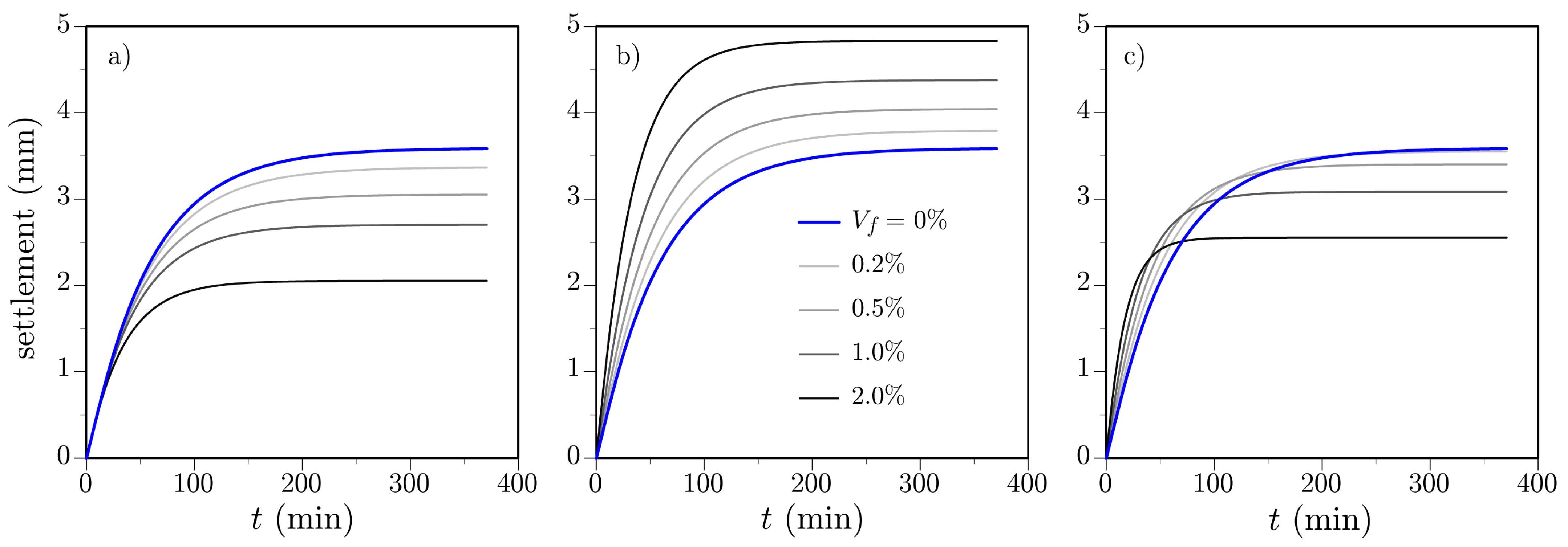
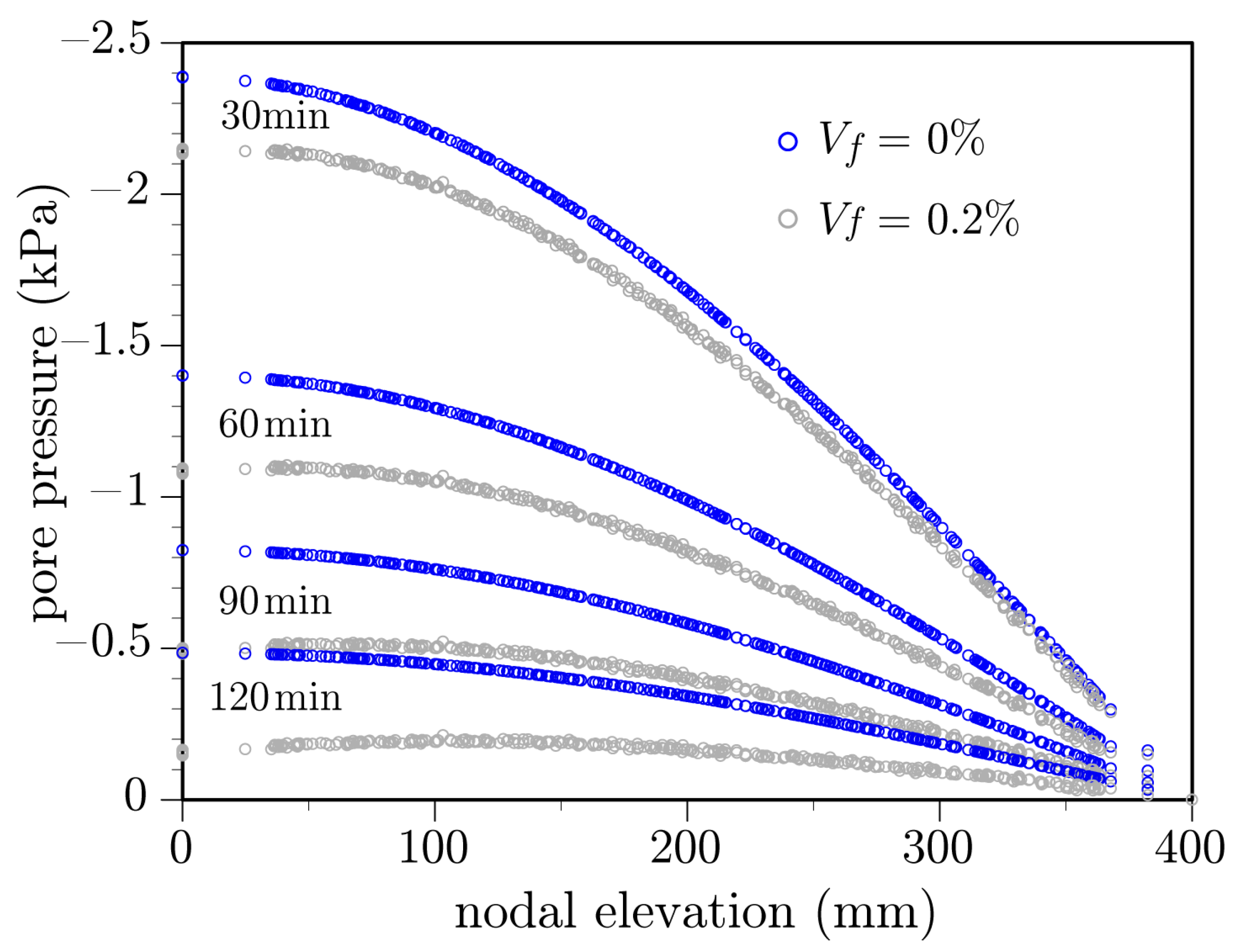
• The proposed model enables study of the relative benefits of introducing short fibers to reduce plastic settlement of concrete. Both the mechanical and transport modifications of the material are considered. The simulation results support some experimental observations that higher fiber content leads to reduced settlement and increased amounts of bleed water due to the stiffness and conductivity enhancements of the fibers, respectively.
• Model extensions and validation efforts, through comparisons with physical test data, are needed to address a variety of practical simulation needs. With respect to the validation efforts, it is difficult to measure some of the model input parameters (e.g., the mechanical and hydraulic conductivity properties of individual fibers within fresh concrete). Such quantities need to be determined, either experimentally or through inverse calculations.

References

1. Naaman, A.E. Fiber Reinforced Cement and Concrete Composites; Techno Press 3000: Sarasota, FL, USA, 2017. [Google Scholar]
2. Naaman, A.E.; Wongtanakitcharoen, T.; Hauser, G. Influence of different fibers on plastic shrinkage cracking of concrete. ACI Mater. J. 2005, 102, 49–58. [Google Scholar]
3. Banthia, N.; Gupta, R. Influence of polypropylene fiber geometry on plastic shrinkage cracking in concrete. Cem. Concr. Res. 2006, 36, 1263–1267. [Google Scholar] [CrossRef]
4. Bentz, D.P. A review of early-age properties of cement-based materials. Cem. Concr. Res. 2008, 38, 196–204. [Google Scholar] [CrossRef]
5. Kalifa, P.; Chéné, G.; Gallé, C. High-temperature behaviour of HPC with polypropylene fibres—From spalling to microstructure. Cem. Concr. Res. 2001, 31, 1487–1499. [Google Scholar] [CrossRef]
6. Liu, X.; Ye, G.; De Schutter, G.; Yuan, Y.; Taerwe, L. On the mechanism of polypropylene fibres in preventing fire spalling in self-compacting and high-performance cement paste. Cem. Concr. Res. 2008, 38, 487–499. [Google Scholar] [CrossRef]
7. Far, B.K.; Zanotti, C. Concrete-concrete bond in Mode-I: A study on the synergistic effect of surface roughness and fiber reinforcement. Appl. Sci. 2019, 9, 2556. [Google Scholar] [CrossRef] [Green Version]
8. Moreno, D.M.; Trono, W.; Jen, G.; Ostertag, C.; Billington, S.L. Tension stiffening in reinforced high performance fiber reinforced cement-based composites. Cem. Concr. Compos. 2014, 50, 36–46. [Google Scholar] [CrossRef]
9. Roy, M.; Hollmann, C.; Wille, K. Influence of fiber volume fraction and fiber orientation on the uniaxial tensile behavior of rebar-reinforced ultra-high performance concrete. Fibers 2019, 7, 67. [Google Scholar] [CrossRef] [Green Version]
10. Nguyen, W.; Bandelt, M.J.; Trono, W.; Billington, S.L.; Ostertag, C.P. Mechanics and failure characteristics of hybrid fiber-reinforced concrete (HyFRC) composites with longitudinal steel reinforcement. Eng. Struct. 2019, 183, 243–254. [Google Scholar] [CrossRef]
11. Xie, P.; Gu, P.; Beaudoin, J.J. Electrical percolation phenomena in cement composites containing conductive fibers. J. Mater. Sci. 1996, 31, 4093–4097. [Google Scholar] [CrossRef]
12. Azhari, F.; Banthia, N. Cement-based sensors with carbon fibers and carbon nanotubes for piezoresistive sensing. Cem. Concr. Compos. 2012, 34, 866–873. [Google Scholar] [CrossRef]
13. Berrocal, C.G.; Hornbostel, K.; Geiker, M.R.; Lofgren, I.; Lundgren, K.; Bekas, D.G. Electrical resistivity measurements in steel fibre reinforced cementitious materials. Cem. Concr. Compos. 2018, 89, 216–229. [Google Scholar] [CrossRef] [Green Version]
14. Hatta, H.; Taya, M. Effective thermal conductivity of a misoriented short fiber composite. J. Appl. Phys. 1985, 58, 2478–2486. [Google Scholar] [CrossRef]
15. Park, K.; Paulino, G.H.; Roesler, J. Cohesive fracture model for functionally graded fiber reinforced concrete. Cem. Concr. Res. 2010, 40, 956–965. [Google Scholar] [CrossRef]
16. Kozicki, J.; Tejchman, J. Effect of steel fibres on concrete behavior in 2D and 3D simulations using lattice model. Arch. Mech. 2010, 62, 465–492. [Google Scholar]
17. Smith, J.; Cusatis, G.; Pelessone, D.; Landis, E.; O’Daniel, J.; Baylot, J. Discrete modeling of ultra-high performance concrete with application to projectile penetration. Int. J. Impact Eng. 2014, 65, 13–32. [Google Scholar] [CrossRef]
18. Kang, J.; Bolander, J.E. Event-based lattice modeling of strain-hardening cementitious composites. Int. J. Fract. 2017, 206, 245–261. [Google Scholar] [CrossRef]
19. Ogura, H.; Kunieda, M.; Nakamura, H. Tensile fracture analysis of fiber reinforced cement-based composites with rebar focusing on the contribution of bridging forces. J. Adv. Concr. Technol. 2019, 17, 216–231. [Google Scholar] [CrossRef]
20. Bolander, J.E.; Berton, S. Simulation of shrinkage induced cracking in cement composite overlays. Cem. Concr. Compos. 2004, 26, 861–871. [Google Scholar] [CrossRef]
21. Bolander, J.E.; Saito, S. Discrete modeling of short-fiber reinforcement in cementitious composites. Adv. Cem. Based Mater. 1997, 6, 76–86. [Google Scholar] [CrossRef]
22. Kawai, T. New discrete models and their application to seismic response analysis of structures. Nucl. Eng. Des. 1978, 48, 207–229. [Google Scholar] [CrossRef]
23. Bolander, J.E.; Saito, S. Fracture analyses using spring networks with random geometry. Eng. Fract. Mech. 1998, 61, 569–591. [Google Scholar] [CrossRef]
24. Nagai, K.; Sato, Y.; Ueda, T. Mesoscopic simulation of failure of mortar and concrete by 3D RBSM. J. Adv. Concr. Technol. 2005, 3, 385–402. [Google Scholar] [CrossRef] [Green Version]
25. Bažant, Z.P.; Tabbara, M.R.; Kazemi, M.T.; Pijaudier-Cabot, G. Random Particle Model for Fracture of Aggregate or Fiber Composites. J. Eng. Mech. 1990, 116, 1686–1705. [Google Scholar] [CrossRef]
26. Schlangen, E.; van Mier, J.G.M. Experimental and numerical analysis of micro-mechanisms of fracture of cement-based composites. Cem. Concr. Compos. 1992, 14, 105–118. [Google Scholar] [CrossRef]
27. Jirásek, M.; Bažant, Z.P. Particle model for quasibrittle fracture and application to sea ice. J. Eng. Mech. ASCE 1995, 121, 1016–1025. [Google Scholar] [CrossRef] [Green Version]
28. Cusatis, G.; Pelessone, D.; Mencarelli, A. Lattice Discrete Particle Model (LDPM) for failure behavior of concrete. I: Theory. Cem. Concr. Compos. 2011, 33, 881–890. [Google Scholar] [CrossRef]
29. Alnaggar, M.; Cusatis, G.; di Luzio, G. Lattice Discrete Particle Modeling (LDPM) of Alkali Silica Reaction (ASR) deterioration of concrete structures. Cem. Concr. Compos. 2013, 41, 45–59. [Google Scholar] [CrossRef]
30. Šavija, B.; Pacheco, J.; Schlangen, E. Lattice modeling of chloride diffusion in sound and cracked concrete. Cem. Concr. Compos. 2013, 42, 30–40. [Google Scholar] [CrossRef]
31. Eliáš, J.; Vořechovský, M.; Skoček, J.; Bažant, Z.P. Stochastic discrete meso-scale simulations of concrete fracture: Comparison to experimental data. Eng. Fract. Mech. 2015, 135, 1–16. [Google Scholar] [CrossRef]
32. Boumakis, I.; di Luzio, G.; Marcon, M.; Vorel, J.; Wan-Wendner, R. Discrete element framework for modeling tertiary creep of concrete in tension and compression. Eng. Fract. Mech. 2018, 200, 263–282. [Google Scholar] [CrossRef] [Green Version]
33. Asahina, D.; Bolander, J.E. Voronoi-based discretizations for fracture analysis of particulate materials. Powder Technol. 2011, 213, 92–99. [Google Scholar] [CrossRef]
34. Berton, S.; Bolander, J.E. Crack band model of fracture in irregular lattices. Comput. Methods Appl. Mech. Eng. 2006, 195, 7172–7181. [Google Scholar] [CrossRef]
35. Asahina, D.; Aoyagi, K.; Kim, K.; Birkholzer, J.T.; Bolander, J.E. Elastically-homogeneous lattice models of damage in geomaterials. Comput. Geotech. 2017, 81, 195–206. [Google Scholar] [CrossRef] [Green Version]
36. Yamamoto, Y.; Isaji, Y.; Nakamura, H.; Miura, T. Collapse simulation of reinforced concrete including localized failure and large rotation using extended RBSM. In Proceedings of the 10th International Conference on Fracture Mechanics of Concrete and Concrete Structure (FraMCoS X), Bayonne, France, 24–26 June 2019. [Google Scholar]
37. Hwang, Y.K.; Bolander, J.E.; Hong, J.W.; Lim, Y.M. Irregular lattice model for geometrically nonlinear dynamics of structures. Mech. Res. Commun. 2020, 107, 103554. [Google Scholar] [CrossRef]
38. Bažant, Z.P.; Oh, B.H. Crack band theory for fracture of concrete. Mater. Struct. 1983, 16, 155–177. [Google Scholar] [CrossRef] [Green Version]
39. Červenka, J.; Červenka, V.; Laserna, S. On crack band model in finite element analysis of concrete fracture in engineering practice. Eng. Fract. Mech. 2019, 197, 27–47. [Google Scholar] [CrossRef]
40. Pan, Y.; Prado, A.; Porras, R.; Hafez, O.; Bolander, J.E. Lattice modeling of early-age behavior of structural concrete. Materials 2017, 10, 231. [Google Scholar] [CrossRef] [Green Version]
41. Nakamura, H.; Srisoros, W.; Yashiro, R.; Kunieda, M. Time-dependent structural analysis considering mass transfer to evaluate deterioration processes of RC structures. J. Adv. Concr. Technol. 2006, 4, 147–158. [Google Scholar] [CrossRef] [Green Version]
42. Grassl, P.; Fahy, C.; Gallipoli, D.; Wheeler, S. On a 2D hydro-mechanical lattice approach for modelling hydraulic fracture. J. Mech. Phys. Solids 2015, 75, 104–118. [Google Scholar] [CrossRef] [Green Version]
43. Grassl, P.; Bolander, J.E. Three-dimensional network model for coupling of fracture and mass transport in quasi-brittle geomaterials. Mater. J. 2016, 9, 782. [Google Scholar] [CrossRef] [PubMed] [Green Version]
44. Fascetti, A.; Oskay, C. Dual random lattice modeling of backward erosion piping. Comput. Geotech. 2019, 105, 265–276. [Google Scholar] [CrossRef]
45. Bažant, Z.P.; Najjar, L.J. Drying of concrete as a nonlinear diffusion problem. Cem. Concr. Res. 1971, 1, 461–473. [Google Scholar] [CrossRef]
46. Lewis, R.W.; Morgan, K.; Thomas, H.R.; Seetharamu, K.N. The Finite Element Method in Heat Transfer Analysis; John Wiley & Sons, Inc.: Hoboken, NJ, USA, 1996. [Google Scholar]
47. Montero-Chacón, F.; Schlangen, E.; Cifuentes, H.; Medina, F. A numerical approach for the design of multiscale fibre-reinforced cementitious composites. Philos. Mag. 2015, 95, 3305–3327. [Google Scholar] [CrossRef]
48. Radtke, F.K.F.; Simone, A.; Sluys, L.J. A partition of unity finite element method for simulating nonlinear debonding and matrix failure in thin fibre composites. Int. J. Numer. Methods Eng. 2011, 86, 453–476. [Google Scholar] [CrossRef]
49. Schauffert, E.A.; Cusatis, G. Lattice Discrete Particle Model for fiber-reinforced concrete. I: Theory. J. Eng. Mech. 2012, 138, 826–833. [Google Scholar] [CrossRef]
50. Caner, F.C.; Bažant, Z.; Wendner, R. Microplane model M7f for fiber reinforced concrete. Eng. Fract. Mech. 2013, 105, 41–57. [Google Scholar] [CrossRef] [Green Version]
51. Luković, M.; Dong, H.; Šavija, B.; Schlangen, E.; Ye, G.; Breugel, K.V. Tailoring strain-hardening cementitious composite repair systems through numerical experimentation. Cem. Concr. Compos. 2014, 53, 200–213. [Google Scholar] [CrossRef]
52. Zhan, Y.; Meschke, G. Multilevel computational model for failure analysis of steel-fiber–reinforced concrete structures. J. Eng. Mech. 2016, 142, 04016090. [Google Scholar] [CrossRef]
53. Kunieda, M.; Ogura, H.; Ueda, N.; Nakamura, H. Tensile fracture process of strain hardening cementitious composites by means of three-dimensional meso-scale analysis. Cem. Concr. Compos. 2011, 33, 956–965. [Google Scholar] [CrossRef]
54. Eddy, L.; Nagai, K. Numerical simulation of beam-column knee joints with mechanical anchorages by 3D rigid body spring model. Eng. Struct. 2016, 126, 547–558. [Google Scholar] [CrossRef]
55. Kuntal, V.S.; Jiradilok, P.; Bolander, J.E.; Nagai, K. Estimation of internal corrosion degree from observed surface cracking of concrete using mesoscale simulation with Model Predictive Control. Comput. Aided Civ. Infrastruct. Eng. 2020, 1–16. [Google Scholar] [CrossRef]
56. Fu, L.; Nakamura, H.; Yamamoto, Y.; Miura, T. Effect of various structural factors on shear strength degradation after yielding of RC members under cyclic loads. J. Adv. Concr. Technol. 2020, 18, 211–226. [Google Scholar] [CrossRef] [Green Version]
57. Ferrara, L.; Ozyurt, N.; di Prisco, M. High mechanical performance of fibre reinforced cementitious composites: The role of “casting-flow induced” fibre orientation. Mater. Struct. 2011, 44, 109–128. [Google Scholar] [CrossRef]
58. Lee, B.Y.; Kang, S.T.; Yun, H.B.; Kim, Y.Y. Improved sectional image analysis technique for evaluating fiber orientations in fiber-reinforced cement-based materials. Materials 2016, 9, 42. [Google Scholar] [CrossRef] [PubMed] [Green Version]
59. Choi, M.S.; Kang, S.T.; Lee, B.Y.; Koh, K.T.; Ryu, G.S. Improvement in predicting the post-cracking tensile behavior of ultra-high performance cementitious composites based on fiber orientation distribution. Materials 2016, 9, 829. [Google Scholar] [CrossRef] [Green Version]
60. Stahli, P.; Custer, R.; van Mier, J.G.M. On flow properties, fibre distribution, fibre orientation and flexural behaviour of FRC. Mater. Struct. 2008, 41, 189–196. [Google Scholar] [CrossRef]
61. Svec, O.; Zirgulis, G.; Bolander, J.E.; Stang, H. Influence of formwork surface on the orientation of steel fibres within self-compacting concrete and on the mechanical properties of cast structural elements. Cem. Concr. Compos. 2014, 50, 60–72. [Google Scholar] [CrossRef]
62. Oesch, T.; Landis, E.; Kuchma, D. A methodology for quantifying the impact of casting A methodology for quantifying the impact of casting procedure on anisotropy in fiber-reinforced concrete using X-ray CT. Mater. Struct. 2018, 51, 1–13. [Google Scholar] [CrossRef]
63. Knop, R.E. Random vectors uniform in solid angle. Commun. ACM 1970, 13, 326–327. [Google Scholar] [CrossRef]
64. Lumelsky, V.J. On fast computation of distance between line segments. Inf. Process. Lett. 1985, 21, 55–61. [Google Scholar] [CrossRef]
65. Cox, H.L. The elasticity and strength of paper and other fibrous materials. Br. J. Appl. Phys. 1952, 3, 72–79. [Google Scholar] [CrossRef]
66. Naaman, A.E.; Namur, G.G.; Alwan, J.M.; Najm, H.S. Fiber Pullout and Bond Slip. I: Analytical Study. J. Struct. Eng. 1991, 117, 2769–2790. [Google Scholar] [CrossRef]
67. Kang, J.; Kim, K.; Lim, Y.M.; Bolander, J.E. Modeling of fiber-reinforced cement composites: Discrete representation of fiber pullout. Int. J. Solids Struct. 2014, 51, 1970–1979. [Google Scholar] [CrossRef] [Green Version]
68. Loh, K.J.; Hou, T.C.; Lynch, J.P.; Kotov, N.A. Carbon nanotube sensing skins for spatial strain and impact damage identification. J. Nondestruct. Eval. 2009, 28, 9–25. [Google Scholar] [CrossRef]
69. Eshelby, J.D. The determination of the elastic field of an ellipsoidal inclusion, and related problems. Proc. R. Soc. 1957, A241, 376–396. [Google Scholar]
70. Hashin, Z.; Shtrikman, S. A variational approach to the theory of the effective magnetic permeability of multiphase materials. J. Appl. Phys. 1962, 33, 3125. [Google Scholar] [CrossRef]
71. Mehta, P.K.; Monteiro, P.J.M. Concrete: Microstructure, Properties, and Materials, 4th ed.; McGraw-Hill Education: Berkshire, UK, 2014. [Google Scholar]
72. Kang, S.T.; Lee, B.Y.; Kim, J.K.; Kim, Y.Y. The effect of fibre distribution characteristics on the flexural strength of steel fibre-reinforced ultra high strength concrete. Constr. Build. Mater. 2011, 25, 2450–2457. [Google Scholar] [CrossRef]
73. Kang, J.; Rypl, R.; Bolander, J.E. Lattice modeling of strain-hardeningcement composites with spatially correlated random fiber distributions. In Proceedings of the 9th RILEM International Symposium on Fiber Reinforced Concrete (BEFIB 2016), Vancouver, BC, Canada, 19–21 September 2016; Banthia, N., di Prisco, M., Eds.; The University of British Columbia: Vancouver, BC, Canada, 2016. [Google Scholar]
74. Powers, T. The Properties of Fresh Concrete; Wiley: New York, NY, USA, 1968. [Google Scholar]
75. Wittmann, F. On the action of capillary pressure in fresh concrete. Cem. Concr. Res. 1976, 6, 49–56. [Google Scholar] [CrossRef]
76. Slowik, V.; Schmidt, M.; Fritzsch, R. Capillary pressure in fresh cement-based materials and identification of the air entry value. Cem. Concr. Compos. 2008, 30, 557–565. [Google Scholar] [CrossRef]
77. Combrinck, R. Cracking of Plastic Concrete in Slab-Like Elements. Ph.D. Thesis, Stellenbosch University, Stellenbosch, South Africa, 2016. [Google Scholar]
78. Slowik, V.; Schmidt, M. Kapillare Schwindrissbildung in Beton: Forschungsbericht zu Ursachen und Auswirkungen sowie zur Vermeidung von Frühschwindrissen; Beuth Verlag GmbH: Berlin, Germany, 2010. [Google Scholar]
79. Combrinck, R.; Boshoff, W.P. Typical plastic shrinkage cracking behaviour of concrete. Mag. Concr. Res. 2013, 65, 486–493. [Google Scholar] [CrossRef]
80. Wang, K.; Shah, S.P.; Phuaksuk, P. Plastic shrinkage cracking in concrete materials—Influence of fly ash and fibers. ACI Mater. J. 2001, 98, 458–464. [Google Scholar]
81. Qi, C.; Weiss, J.; Olek, J. Characterization of plastic shrinkage cracking in fiber reinforced concrete using image analysis and a modified Weibull function. Mater. Struct. 2003, 36, 386–395. [Google Scholar] [CrossRef]
82. Wongtanakitcharoen, T.; Naaman, A.E. Unrestrained early age shrinkage of concrete with polypropylene, PVA, and carbon fibers. Mater. Struct. 2006, 40, 289–300. [Google Scholar] [CrossRef]
83. Fontana, P.; Pirskawetz, S.; Lura, P. Plastic shrinkage cracking risk of concrete–Evaluation of test methods. In Proceedings of the 7th RILEM International Conference on Cracking in Pavements, Delft, The Netherlands, 20–22 June 2012; Springer: Dordrecht, The Netherlands, 2012; pp. 591–600. [Google Scholar]
84. Sivakumar, A.; Santhanam, M. A quantitative study on the plastic shrinkage cracking in high strength hybrid fibre reinforced concrete. Cem. Concr. Compos. 2007, 29, 575–581. [Google Scholar] [CrossRef]
85. Kronlöf, A.; Leivo, M.; Sipari, P. Experimental study on the basic phenomena of shrinkage and cracking of fresh mortar. Cem. Concr. Res. 1995, 25, 1747–1754. [Google Scholar] [CrossRef]
86. Terzaghi, K. Theoretical Soil Mechanics; John Wiley and Sons: Hoboken, NJ, USA, 1943. [Google Scholar]
87. Biot, M.A. General theory of three-dimensional consolidation. J. Appl. Phys. 1941, 12, 155–164. [Google Scholar] [CrossRef]
88. Lewis, R.W.; Schrefler, B.A. The Finite Element Method in the Static and Dynamic Deformation and Consolidation of Porous Media; John Wiley: Hoboken, NJ, USA, 1998. [Google Scholar]
89. Tan, T.S.; Wee, T.H.; Tan, S.A.; Tam, C.T.; Lee, S.L. A consolidation model for bleeding of cement paste. Adv. Cem. Res. 1987, 1, 18–26. [Google Scholar] [CrossRef]
90. Kwak, H.G.; Ha, S. Plastic shrinkage cracking in concrete slabs. Part I: A numerical model. Mag. Concr. Res. 2006, 58, 505–516. [Google Scholar] [CrossRef]
91. Kwak, H.G.; Ha, S. Plastic shrinkage cracking in concrete slabs. Part II: Numerical experiment and prediction of occurrence. Mag. Concr. Res. 2006, 58, 517–532. [Google Scholar] [CrossRef]
92. Kwak, H.G.; Ha, S.; Weiss, W.J. Experimental and numerical quantification of plastic settlement in fresh cementitious systems. J. Mater. Civ. Eng. 2010, 22, 951–966. [Google Scholar] [CrossRef]
93. di Luzio, G.; Cusatis, G. Solidification-microprestress-microplane (SMM) theory for concrete at early age: Theory, validation and application. Int. J. Solids Struct. 2013, 50, 957–975. [Google Scholar] [CrossRef] [Green Version]
94. Yu, P.; Duan, Y.H.; Chen, E.; Tang, S.W.; Hanif, A.; Fan, Y.L. Microstructure-based homogenization method for early-age creep of cement paste. Constr. Build. Mater. 2018, 188, 1193–1206. [Google Scholar] [CrossRef]
95. Zhou, W.; Duan, L.; Tang, S.W.; Chen, E.; Hanif, A. Modeling the evolved microstructure of cement pastes governed by diffusion through barrier shells of C-S-H. J. Mater. Sci. 2019, 54, 4680–4700. [Google Scholar] [CrossRef]
96. Gawin, D.; Pesavento, F.; Schrefler, B.A. Hygro-thermo-chemo-mechanical modelling of concrete at early ages and beyond. Part I: Hydration and hygro-thermal phenomena. Int. J. Numer. Methods Eng. 2006, 67, 299–331. [Google Scholar] [CrossRef]
97. Kim, J.M.; Parizek, R.R. A mathematical model for the hydraulic properties of deforming porous media. Groundwater 1999, 37, 546–554. [Google Scholar] [CrossRef]
98. Kang, J.; Bolander, J.E. Flow in fibrous composite materials: Numerical simulations. In Proceedings of the Computational Modeling of Concrete and Concrete Structures (EURO-C 2018), Bad Hofgastein, Austria, 26 February–1 March 2018. [Google Scholar]
99. Pan, Y. Lattice Modeling of Volumetric Variation of Cementitious Materials at very Early Age. Ph.D. Thesis, Department of Civil and Environmental Engineering, University of California, Davis, CA, USA, 2018. [Google Scholar]
Figure 1. Lattice model: (a) domain discretization based on Delaunay and Voronoi tessellations; (b) mechanical lattice element i j based on the rigid-body-spring concept; and (c) conductive lattice element i j .
Applsci 11 00184 g001
Figure 2. (a) Fiber inclusions within unit cell; (b) discretization of fiber cross-section; and (c) periodic representation of fibers that intersect boundaries.
Applsci 11 00184 g002
Figure 3. Semi-discrete representation of fiber I J : (a) elemental pathway with enhanced conductivity; and (b) length h f used for conductivity calculations of element i j .
Applsci 11 00184 g003
Figure 4. Planar lattice modeling of fiber inclusions: (a) discrete representation of a single fiber aligned with the direction of flow; (b) corresponding potential distribution; (c) potential distribution based on semi-discrete fiber approach; and (d) application of semi-discrete approach to multiple fibers.
Applsci 11 00184 g004
Figure 5. Profile view of fiber distribution within the 3D unit cell.
Applsci 11 00184 g005
Figure 6. Flow through a cluster of conductive fibers embedded within a lowly conductive matrix. The fiber aspect ratio l f / d f = 30.
Applsci 11 00184 g006
Figure 7. Relationship between fiber content and conductivity of the composite material according to two effective medium theories (for conductivity ratio σ f / σ m = 1000 and aspect ratio l f / d f = 50).
Applsci 11 00184 g007
Figure 8. (a) Composite conductivity values based on discrete (volumetric) fiber models. Seven nominally identical, randomly generated models were tested for each V f value; and (b) dependence of simulated conductivity measurements on the orientation of fibers with respect to the direction of the electric field.
Applsci 11 00184 g008
Figure 9. Relative number of nodes for discretizing the fiber composite volume.
Applsci 11 00184 g009
Figure 10. (a) Composite conductivity values based on semi-discrete fiber models. Seven nominally identical, randomly generated models were tested for each V f value; and (b) dependence of simulated conductivity measurements on the orientation of fibers with respect to the direction of the electric field.
Applsci 11 00184 g010
Figure 11. Change in resistance of the numerical specimen under sinusoidal mechanical loading.
Applsci 11 00184 g011
Figure 12. Discretization for VCLM analyses: (a) two-dimensional; and (b) three-dimensional representations of the virtual specimen.
Applsci 11 00184 g012
Figure 13. Comparison of top layer settlement with time among multi-dimensional VCLM meshes and original planar FE model of Kwak et al. [92].
Applsci 11 00184 g013
Figure 14. Nodal values of vertical displacement and pore pressure at differing times after casting.
Applsci 11 00184 g014
Figure 15. Influence of fiber dosage on surface layer settlement considering: (a) stiffness contributions of fibers; (b) conductivity contributions of fibers; and (c) combined stiffness and conductivity effects of fibers.
Applsci 11 00184 g015
Figure 16. Effect of stiffening fiber dosage on the vertical displacement of all nodal points at t = 150 min.
Applsci 11 00184 g016
Figure 17. Influence of fiber dosage on the development of pore pressure distribution over time.
Applsci 11 00184 g017
Figure 18. Pore pressure distribution and nodal value profile at t = 90 min for: (a) V f = 0%; and (b) V f = 0.2%.
Applsci 11 00184 g018