Abstract
Recent advancements in sensor, mobile computing, and wireless communication technologies is creating new opportunities to effectively exploit real-time traffic data. Onboard vehicles collect, process, simulate traffic states in a distributed fashion and a local transportation management center coordinates the overall simulation with an optimistic execution technique. Such a distributed approach can provide more up-to-date and robust estimates with decreased communication bandwidth requirements and increased computing capacity. This paper proposes an online ad hoc distributed simulation. The physical operating platform for the model including operating system, communicational middleware, and traffic simulation model are described. Also, this paper investigates the analytical background of rollback process of the proposed ad hoc distributed simulation model. Flow rate diagram and cumulative number of vehicle diagram show that the overall system simulation speed and estimate accuracy may differ significantly as a function of the selected threshold.
1. Introduction
Transportation impacts every aspect of daily life. For many decades, efforts to improve transportation have been made to ensure quality of life and higher standards of living. However, use of real-time traffic data into our surface transportation system has not been fully accomplished. Recent advancements in sensor, mobile computing, and wireless communication technologies is creating new opportunities to effectively exploit real-time traffic data. Onboard vehicles collect, process, simulate traffic states in a distributed fashion and a local transportation management center coordinates the overall simulation with an optimistic execution technique. Such a distributed approach can provide more up-to-date and robust estimates with decreased communication bandwidth requirements and increased computing capacity [1].
As roadside and in-vehicle sensors are deployed under the Connected Vehicle and autonomous vehicle environments, an increasing variety of traffic data is becoming available in real-time. This real-time traffic data can be shared through wireless communication and used for other purposes, which creates an opportunity for mobile computing and online traffic simulations [2,3].
However, online traffic simulations require faster than real-time running speed with high simulation resolution, since the purpose of the simulations is to provide immediate future traffic forecast based on real-time traffic data. Simulating at high resolution is often too computationally intensive to process a large-scale network on a single processor in real-time. To mitigate this limitation an online ad hoc distributed simulation with optimistic execution is proposed in this paper.
The goal of this paper is to develop an online ad hoc distributed traffic simulation system based on optimistic execution. It is envisioned that in the proposed distributed traffic simulation framework, each in-vehicle simulation models a small portion of the overall network and provides detailed traffic state information. Traffic simulation and data processing are performed in a distributed fashion by multiple vehicles. Each in-vehicle simulation is designed to run in real-time and update its estimates when it is necessary. A communication middleware is used for the distributed simulation to perform on multiple platforms. A communication middleware developed based on object-oriented client/server technology as a parallel effort is integrated with traffic simulation. This integration manages the distributed network to synchronize the predictions among logical processes. Space-Time Memory management scheme is implemented into a transportation simulation approach. A local central server receives the traffic states from multiple in-vehicle simulations. Traffic estimates are not guaranteed to be received in time stamp order, since in-vehicles simulations run concurrently. Also, a traffic state can be projected by multiple in-vehicle simulations. A mechanism is needed to coordinate the transmitted data, combine values into a composite value, and save in Space-Time Memory. To handle the data received from all participating vehicles, an optimistic (rollback-based) synchronization protocol is developed. Optimistic execution inspired by Time Warp can mitigate the synchronization problem allowing each logical process to execute asynchronously [4]. This approach provides increased computing capacity with a time-synchronized approach.
This paper will review the previous research regarding vehicular ad hoc network and parallel and distributed simulation technologies associated with vehicular ad hoc network. To run a large simulation with fast speed, parallel and distributed simulation has been used in transportation area. Generally, parallel and distributed simulations are differentiated by the geographical distribution, the composition of the processors used, and the network to interconnect the processors. Also, two popular approaches for the synchronization were discussed; (1) conservative time synchronization and (2) optimistic time synchronization.
In transportation area, previous research efforts to divide a large-scale traffic simulation over different processors can be classified into two approaches; (1) task parallelization and (2) domain decomposition. Most of the research in traffic simulation followed the conservative time synchronization. However, in this conservative time synchronization approach, speed of the entire simulation is dependent on the slowest processor, since all processors need to be synchronized with respect to simulation time. To evaluate the potential of concurrent simulation run by geographically distributed heterogeneous processors, this paper proposes an ad hoc distributed approach based on optimistic time synchronization. In this optimistic time synchronization approach, geographically distributed heterogeneous processors are allowed to run concurrently while obeying Local Causality Constraint (LCC).
2. Literature Review
Parallel and distributed simulation refers to technologies that enable a simulation model to execute on multiple processors [4]. Its benefit includes reduced execution time, larger model scale, and integration with other simulators [5,6,7]. Parallel and distributed simulations can be distinguished by the geographical distribution, the composition of the processors used, and the network to interconnect the processors. While the processors in a parallel simulation are homogeneous machines and located in close physical proximity, the processors in distributed simulation are often composed of heterogeneous machines that may be geographically distributed (Table 1). For communication between processors, parallel simulation uses customized interconnection switches and distributed simulation uses widely accepted telecommunication standards including LAN (Local Area Network) and WAN (Wide Area Network) [4].

Table 1.
Parallel and distributed computing [4].
When a simulation program is distributed over multiple processors in parallel and distributed simulation, several LPs (logical processes) execute simulations concurrently. In such simulations time stamp ordered processing is not guaranteed, as in a sequential execution on a single machine. Errors resulting from out-of-order processing are referred as causality errors. Out-of-order execution must be prevented to ensure the parallel and distributed simulation produces the same results as a sequential execution. To avoid causality errors, synchronization algorithms are required which refer to the coordination of simulation processes in a time stamp order to complete a task. Under the synchronization algorithms, LPs execute simulations while obeying a rule known as Local Causality Constraint (LCC). Two different synchronization approaches have been proposed to satisfy the local causality constraint, conservative execution, and optimistic execution [4,5,6,7,8,9,10,11,12]. LPs in conservative synchronization protocols strictly avoid violating LCC. Each LP only advances when it is safe to proceed after satisfying LCC. However, optimistic algorithms assume “optimistically” that there are no causality errors and allow LPs to process asynchronously. LCC violation can occur, since optimistic execution does not determine when it is safe to proceed for each LP. Instead, when a causality error is detected, a mechanism to recover is provided in the optimistic approach. Once a causality error is detected simulation states prior to the causal violation are recalled and the simulation is executed forward from that state, with the LCC violation corrected.
The operation of recovering a previous state is known as a rollback and this recovering process requires state-saving and anti-message. State-saving stores state variables values prior to an event computation. Two widely used techniques for state-saving are Copy state-saving and Incremental state-saving. Copy state-saving creates an entire copy of the modifiable state variables, whereas Incremental state-saving records (1) the address of the state variables that was modified and (2) the value of the state variable prior to the modification. If a small number of state variables are changed, incremental state-saving is more efficient, reducing the time and memory overheads. However, incremental state-saving does not perform well when most of the state variables are modified by each event. Infrequent state-saving is an alternative to reduce the overheads by decreasing frequency of LP state-saving [13]. When a rollback event happens, the simulation state being rolled back may have sent messages which are not consistent with the rolled back state. Those messages have to be annihilated or cancelled in the anti-messaging process [4].
Among many possible ways of dividing a large-scale simulation over different processors, two approaches are popular; (1) task parallelization and (2) domain decomposition [14,15] as summarized in Table 2. MITSIM, DynaMIT, and DYNASMART are using task parallelization for faster processing [16,17,18] and different modules of a traffic simulation package (vehicle generation, signal operation, routing, etc.) are assigned to different computers in those models. This approach is conceptually straightforward and fairly insensitive to network bottlenecks. On the other hand, domain decomposition is splitting a simulation with respect to time or space. For time decomposition, the domain is partitioned into several time intervals and each processor is responsible for running simulation of an assigned time interval. Space decomposition is more popular for traffic simulation. In this scheme, a simulation network is divided into multiple sub-networks and each sub-network is assigned to a different machine.
Table 2.
Parallel and distributed computing in traffic simulation.
Several traffic simulation models have implemented this domain decomposition approach to split computational loads over different computers in order to achieve fast running speed. The models include Transportation Analysis and Simulation System (TRANSIMS) [19,20,21], Advanced Interactive Microscopic Simulator for Urban and Non-Urban Networks (AIMSUN) [22,23], and Parallel Microscopic Simulation (Paramics) [24,25].
TRANSIMS is an agent-based transportation forecast model developed by Los Alamos National Laboratory. It is a micro-simulation-based model using cellular automata (CA) approach to simulate second-by-second movements of every vehicle in a large metropolitan area. In TRANSIMS the network can be partitioned into tiles of similar size and boundary information is exchanged between processors for global synchronization [19,20,21]. AIMSUN2 is a microscopic simulation program originally developed as a sequential version, but later parallel computing architectures AIMSUN2/MT (the multi-thread parallelized AIMSUN2) were added. For distributed simulation implementation, a network is divided into layers, blocks, and entities. AIMSUN simulates each vehicle based on lane changing and car following model at the level of the entity (section and junction entity) which are updated at every time step. Entities updated together are grouped into blocks that may be allocated to a single thread. Blocks which need to be updated simultaneously by threads are grouped into a layer. Threads can be executed in parallel by the multiple machines. It was reported that the parallel AIMSUN2 operating on a SUN SPARC station with four processors completed a network simulation consisting of 561 sections and 428 junctions 3.5 times faster than its sequential version [22,23].
PARAMICS (PARAllel MICroscopic Simulation) is a suite of microscopic traffic simulation tools. Cameron et al. [24,25] implemented data parallel programming in Paramics. In their study, multiple simple processors connected in a tightly coupled network executed the same code while with their own input data. Researchers at the National University of Singapore [26] divided the whole network and each sub network was dedicated to a different processor. To maintain the spatial connectivity between regions simulated separately vehicles were transferred to the next processor when they cross the network boundary. The method was implemented on a hypothetical grid-type network with over 150 sq. km, 500 nodes, 1000 links and 72 signalized intersections. Their results showed speed increase from 1.50 to 2.25 times when using two processors and from 1.75 to 3.75 times when using three processors, compared with the speed of simulation without parallel execution. Liu et al. [14] have developed a distributed modeling framework with low-cost networked PCs. Windows Sockets were used as the communication middleware to transfer vehicle information and synchronize the simulation time between the client controller and server simulators. Researchers at the University of California, Irvine [27] developed ParamGrid as a scalable and synchronized framework. They distributed the simulation across low-cost personal computers (PCs) connected by local area network (LAN). A large traffic network was divided into a grid of smaller, rectangular sub-networks. Each sub-network was called a tile and ran on a single-process simulator on a single PC. They developed methodologies to transfer vehicles across tiles and synchronize the simulation time globally using CORBA middleware. They found the simulation performance increased approximately linearly with the number of added low-cost processors.
Bononi et al. [28] proposed Mobile Wireless Vehicular Environment Simulation (MoVES) as a scalable and efficient framework for the parallel and distributed simulation of vehicular ad hoc networks. MoVES was implemented on the ARTIS (Advanced Run Time Infrastructure System) simulation middleware which partially adopted the High Level Architecture (HLA) standard IEEE 1516 and supported conservative time management based on time-stepped approach. They developed solutions for communication overhead reduction and computational/communicational load balancing. Their vehicular model followed a microscopic approach including car following model. However, lane changing policies were not implemented. Their performance analysis demonstrated that MoVES had better performance in scalability, efficiency, and accuracy.
Sippl et al. [29] developed a distributed real-time traffic simulation for autonomous vehicle testing in urban environments. In their model, the synchronization of the Automotive Data and Time Triggered Framework instance and the traffic simulation in Virtual Test Drive is done by the connection toolbox to synchronize Electronic Control Unit and Runtime Data Bus/Simulation Control Protocol data exchange. Mastio et al. [30] proposed distributed agent-based traffic simulations and Raghothama and Meijer [31] developed a distributed, integrated, and interactive traffic simulations. In their model, all the components are distributed and communicate over the network using TCP/IP or UDP. The Data/Control API, the Time Synchronization API, access control to the database and other services such as logic for procedural modeling and so on are implemented using Microsoft’s Web Communication Framework (WCF). Chan et al. [32] developed Mobiliti, a proof-of-concept simulator enabling distributed memory parallelism with an asynchronous execution strategy. Mobiliti was built on top of the Devastator parallel discrete event simulation runtime.
3. Model Development
3.1. Model Platform
The model is comprised of one server and multiple LPs (logic processes). Each LP represents an in-vehicle simulator. To provide for realistic testing each LP uses a separate laptop computer. All computers are equipped with a middleware communication program and a simulation script cod-ed in Microsoft Visual. NET language. The script controls the traffic simulation (VISSIM®, Karlsruhe, Germany) execution (e.g., advancement of time steps, rollback implementation, etc.) and aggregation of simulation output while the middleware facilitates communication between the server and other LPs. The area modeled by each LP covers only a small portion of the overall network. The simulation results, after some aggregation to be discussed in a subsequent section, are sent to the server. A detailed architecture of the model is depicted in Figure 1.
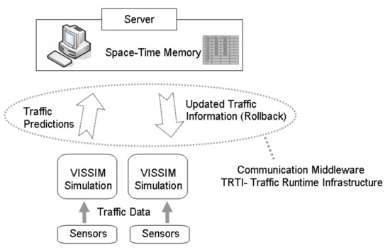
Figure 1.
System architecture.
3.2. Ad Doc Data Process
Ad hoc distributed simulation is a collection of logical processes, LP1, LP2, LP3, …, LPn, which share a global state G that contains object instances G1, G2, G3, …, Gm. The global object instances are saved in Space-Time Memory (STM) inside the server (Figure 1), and synchronized in an optimistic fashion. All the notations described in this study are summarized in Table 3. Once LPi publishes which denotes local state estimates of LPi on link j at simulation time k to the server (m; data type and p; link type), the estimates are transferred from LPi to the message queue located inside the server. The message queue contains traffic data of different links at different simulation times from multiple LPs in the order of time when the message is received. The server processes messages from the message queue in FIFO (first in first out) order by local-to-global transition function . This function converts the local state estimates to global variables. In other words,
where represents global variables on link j at simulation time k generated by LPi with m as data type and p as link type.
Table 3.
Local and global process notation summary.
When the server receives any data from LPi, the composition function aggregates the values of into one global instance . Specifically,
For example, global state instances; , , , , and can be calculated based on the set of .
where n represents all available number of estimates of link j as an internal link at simulation time k.
It is noted that in the calculation of global state instances that only data from LP internal simulation links is used. Inbound and outbound link data is excluded from the aggregation process as they may poorly represent the actual traffic conditions. For example, inbound link traffic performance (travel time, delay, and queue length) may not be accurately modeled as the vehicle arrival headway distribution at the entry point of inbound link may differ from the real traffic pattern on the link. For example, entry link data will not reflect platoon characteristics of arriving vehicles due to upstream intersections not reflected in the model. When considering outbound links, it is noted that vehicles may exit the outbound link regardless of the actual traffic conditions of the link. For instance, when traffic constraints outside the boundaries of the LP simulation result in a spillback of congestion into the region being modeled this spillback will not be reflected in the model. As they have no knowledge of downstream traffic condition, vehicles on the LP simulation may exit the link at free flow speed, providing inaccurate traffic estimates. As discussed later, to address this situation, outbound link speed is controlled to meter the outflow rate from the LP simulation model Thus, upstream internal link behavior will reflect the spillback due to a bottleneck outside the modeled area however the outbound link itself is being artificially manipulated to capture this impact, resulting in its data not being suitable for the global aggregation. More details are discussed in later section on how to represent these intermitted capacity bottlenecks on outbound links and the link speed selection process to meter vehicles.
The server keeps track of all available estimates. represents global state on link j at simulation time k at wall-clock time l with data type m. Two attributes of the ad hoc distributed system estimate are considered (1) length of prediction horizon, i.e., how far in advance of the current wall-clock time the system provides estimates and (2) how accurate the estimates are at specific prediction horizon, i.e., how accurate is the estimate. For example, the following analysis would be available. Suppose at 7:00 AM wall-clock time the system was able to predict until 7:30 AM simulation time and its estimates regarding 10 min period between 7:20 AM simulation time and 7:30 AM simulation time over-estimated by 15%. However, at 7:10 AM wall-clock time with more updated information the system was able to provide the same time period estimates (7:20 AM–7:30 AM simulation time) with better accuracy (5% difference).
Lastly, global-to-local transition function is called when any LPs need to roll back in order to revise its estimates with updated information. This function converts the global object instances to local state, i.e.,
Whenever this function is called, , aggregated value from the estimates of the LPs on link at simulation time , is converted to the local instance for LPi. Then, is used as new input to revise its estimates.
3.3. Rollback Detection
When the server receives estimates from logical process LPi it determines whether a rollback should be triggered for any LPs based on rollback detection function . The rollback detection function compares the flow rate estimates of each LP with the corresponding global instances in the Space-Time Memory and decides which LP needs to renew its estimates. Since LPs model their own network portions of interest and their model networks overlap, each link can be simulated by multiple LPs. Also, the link can be an inbound, outbound, or internal link depending on the network configuration of each LP.
Consider link j, a link which some LPs have as an inbound link, some as an outbound link, and some as an internal link of their own network simulations. Whenever there is an update on the global instance, in the Space-Time Memory, the server checks the difference between and estimates on link j as boundary links (inbound link or outbound link) for the individual LPs that is or . If the difference is greater than a given threshold , then the estimates of the corresponding LP are considered invalid and a rollback is issued from the server.
Consider LPs which have link j as an outbound link. They only model the upstream area of link j, not including downstream area of link j in their network. Since link j is the end link of the network, vehicles on link j exit the network at free flow speed unless there is an outflow constraint. In this case, they may not have a good estimate on link j when the downstream traffic condition outside the boundaries results in a spillback of congestion into the network being modeled. Thus, the traffic condition on link j needs to be adjusted to reflect the spillback traffic condition. On the other hand, LPs which have link j as an inbound link and generate vehicles at a pre-determined flow rate may not represent traffic condition well when a sudden change in incoming traffic is predicted outside of the network boundaries. In this case, input rate on link j is adjusted based on which is included in rollback messages sent from the server.
When the simulation time k is far ahead from the current wall-clock time, is calculated from the LP estimates which are available in the Space-Time Memory at the time period when the server checks . Therefore, it is expected that rollback statistics would vary depending on how many LPs are contributing to the aggregated global values. The number of LPs contributing to the aggregated global values is determined by geographical distributions of LP locations.
3.4. Anti-Messaging
Optimistic synchronization algorithm in an online ad hoc distributed simulation can distribute data through all LPs and allow independent running of LPs. Anti-messaging for invaliding estimates and synchronizing valid estimates are essential for reliable data management and efficient simulation speed. To ensure the accuracy of the global estimates, global instances should be only aggregated using currently valid estimates and invalid estimates should be removed from the Space-Time Memory and its message queue in the server.
If the server detects rollback on LPi at simulation time k, it means the estimates of LPi regarding simulation time k and thereafter (for example, LPi,j,k, LPi,j,k + 1, LPi,j,k + 2, …) are not valid and should be eliminated. The server removes all estimates of LPi from the simulation time k and thereafter from its Space-Time Memory (where already processed data is saved) and the message queue (where received but not-processed data is located). After removing estimates of LPi, the server delivers a rollback message to LPi. The message contains new state value , simulation time, link number and identity of the logical process.
4. Traffic Update from Rollback
In the proposed ad hoc distributed simulation rollback process enables the simulation to adapt to new traffic states and update its own estimates if necessary. The traffic update has two process-es; (1) updating downstream states based on upstream traffic information and (2) updating up-stream traffic conditions according to downstream states.
Consider two LPs which are simulating the network regions as shown in Figure 2. LP 1 models the left side of the network (Gray area) and LP 2 simulates the right part of the network (Black dotted box). Each LP starts its simulation using historical average flow rate as an initial input. Suppose that while the two LPs are projecting future traffic states of their own network, the server receives new information from the other LPs. Further suppose that the difference between the flow from the server and input rate of LP 1 on Link A exceeds a given threshold at some wall-clock time (either present or future estimate). The server will detect a rollback and deliver a rollback message which contains rollback logical process ID information, rollback link number, rollback simulation time, new average link speed, new average flow rate. Once LP 1 receives this rollback message, LP 1 will update its simulation with this new flow rate by undertaking a rollback and publishes new traffic estimates on the links in-side its network to the server. These updated estimates from LP 1 will be transmitted to the server and the Space-Time Memory in the server will be updated accordingly.
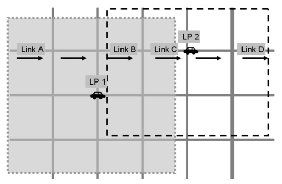
Figure 2.
Two logical process examples.
To provide additional detail the following is a specific potential example of the preceding general discussion. Assume at wall-clock time 7:00 AM, LP 1 starts its simulation based on 300 veh/hr/ln input flow rate on Link A. At wall-clock time 7:10 AM, its prediction horizon extends to 8:00 AM simulation time. However, new information arrives to the Space-Time Memory in the server at wall-clock 7:10 AM forecasting that a 600 veh/hr/ln input rate on Link A is expected at 7:25 AM simulation time (15 min future from the current wall-clock time 7:10 AM). The server compares this new 600 veh/hr/ln input rate with the initial 300 veh/hr/ln input rate which LP 1 has reported to the server and was saved in the Space-Time Memory. Since the 300 veh/hr/ln difference exceeds the assumed current threshold and this new 600 veh/hr/ln input rate is regarded as a valid data, the server issues a rollback to LP 1 and sends the new traffic information. Immediately after receiving the rollback message, LP 1 restores its 7:25 AM simulation state and continues to renew its estimates of 7:25 AM simulation time and thereafter with the updated input data at the current wall-clock time 7:10 AM. Two minutes (wall-clock time) later, at wall-clock time 7:12 AM, LP 1′s prediction horizon reaches 7:35 AM simulation time and its updated estimates are sent to the server. After updating its Space-Time Memory with the new estimates, the server checks if there are any threshold violations. At the current wall-clock time 7:12 AM, the server realizes that increased traffic volume is expected to reach Link B at 7:35 AM simulation time and the flow rate difference between the estimates of LP 1 and input rate of LP 2 surpasses the threshold, causing a rollback on LP 2. With the same method, the server sends a rollback message to LP 2 regarding new traffic information at 7:35 AM simulation time (23 min future from the current wall-clock time 7:12 AM). After updating its input data of 7:35 AM simulation time at the 7:12 AM wall-clock time, LP 2 will continue its simulation and send new estimates of 7:35 AM simulation time and thereafter. The server will update its Space-Time Memory and check the rollback violations every time it receives estimates from any LP.
5. Graphical Analysis and Empirical Analysis
A graphical analysis for speed selection of outflow control is conducted as well as an empirical solution similar to analysis in [33,34]. Suppose that LP 1 and LP 2 are running the ad hoc simulation (Figure 2) with a rollback threshold ( = 200 veh/hr/ln). LP 1 has estimated the average flow rate on Link B until 7:20 AM simulation time would be 120 veh/hr/ln and a sudden flow increase would occur at 7:20 AM simulation time to 600 veh/hr/ln (Figure 3). Further suppose LP 2 uses 120 veh/hr/ln as an initial input flow rate on Link B until it receives updated information regarding the flow change. Even though LP 1 sends a higher flow rate of 7:21 AM simulation time traffic state to the server on Link B, the 4 min flow rate average (240 veh/hr/ln) does not warrant a rollback immediately in the server, since the difference between 240 veh/hr/ln (the 4 min flow rate average by LP 1) and 120 veh/hr/ln (the current input rate of LP 2) is smaller than the given threshold (: 200 veh/hr/ln). However, LP 1′s simulation advances one more simulation minute and LP 1 sends a much higher average flow rate 360 veh/hr/ln at 7:22 AM simulation time. The server compares the difference between 360 veh/hr/ln and 120 veh/hr/ln (the current input rate of LP 2) and sends a rollback message to LP 2, since the difference is greater than the given threshold. Similarly, the difference of 7:23 AM simulation time traffic states (difference between 480 veh/hr/ln by LP 1 and 360 veh/hr/ln, the new input rate for LP 2) is not large enough to force a rollback. One more simulation minute later, LP 2 needs to alter its input flow rate again when the 4 min flow rate average at 7:24 AM simulation time traffic state is greater than 360 veh/hr/ln (the new input rate for LP 2) by more than the given threshold (: 200 veh/hr/ln).
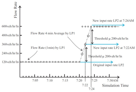
Figure 3.
Flow rate diagram for ad hoc distributed simulation.
A rollback is processed whenever the difference between estimates is greater than the given threshold. This implies the system is dependent on the size of threshold. For example, if the size of threshold becomes smaller, then the system would have more rollbacks, which implies more computational overheads although generally higher agreements between LP estimates across the network. On the other hand, a larger threshold is expected to reduce the computational overheads although may result in higher discrepancies between the LPs.
Figure 4 demonstrates cumulative number of vehicles served on Link B. A(t) represents the cumulative arrivals on Link B in LP 1 and D(t) corresponds to Link B cumulative departure in LP 2 (i.e., cumulative number of entering vehicles on LP 2).
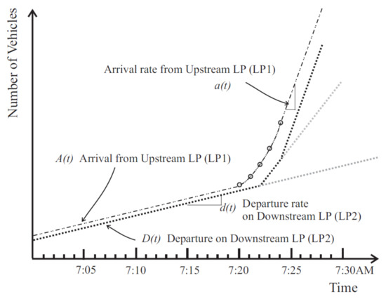
Figure 4.
Cumulative number of vehicle diagram for ad hoc distributed simulation.
As seen in Figure 3, (1) LP 1 sends its traffic estimates to the server and the arrival flow rate from upstream LP 1 is constant as a(t) from simulation time 7:00 AM to 7:20 AM, (2) downstream LP 2 continues its simulation with the departure flow rate equal to d(t), (3) the estimated arrival flow rate from upstream LP 1 begins to increase after 7:20 AM simulation time and the information is sent to the server and saved in the Space-Time Memory, (4) when the arrival rate of 7:22 AM simulation time is sent to the server, the difference between a(t) and d(t) is greater than the given threshold, which prompts the first rollback by the server, (5) the server invalidates traffic states of simulation time 7:22 AM and after (gray dotted line) provided by LP 2 in its Space-Time Memory, (6) the server also sends the new arrival rate information to LP 2, and (7) after receiving the rollback message with the updated flow rate, LP 2 rolls back to simulation state of 7:22 AM simulation time and renews its simulation. Similarly, LP 2 processes another rollback at 7:24 AM.
A drawback of the current threshold method may also be seen in this analysis. A rollback occurs where the slope difference of two curves, i.e., the difference between a(t) and d(t), is greater than the given threshold, since the rollback comparison is based on the point flow rate difference (i.e., absolute flow difference at a time instance, not cumulative difference) in the proposed model. For example, 100 veh/hr/ln arrival rate and 150 veh/hr/ln departure rate with 100 veh/hr/ln threshold does not warrant a rollback in the proposed model, even though 50% more vehicles (50 vehicles) would be generated over an hour. While difference in cumulative vehicle counts would be a good potential measure to detect changes in traffic conditions, it would require additional system measurements, such as counting the number of vehicles entering and exiting the network. Furthermore, the proposed system is associated with numerous rollbacks across the network during the simulation time period. Therefore, the impact of system overhead would need to be considered in collecting cumulative vehicle counts.
As discussed earlier, downstream traffic information is transmitted to upstream LPs in congested traffic conditions. To accomplish this transmission, the outflow rate on the exiting link of the upstream LPs is controlled by changing speed of vehicles on the link. This is required as the simulation model (VISSIM®) has no direct means to throttle the flow rate on an unconstrained link. A question concerning selection of the speed to apply in order to meter the same number of vehicles with downstream LPs is addressed in this section.
Suppose the current 4 min average flow rate which is stored in the Space-Time Memory is calculated as an average of Flow A and Flow B in Figure 5. To process the average flow rate—Flow D (which is , i.e., the average of Flow A and Flow B) in upstream LP, new speed needs to be applied on Link C of the upstream LP in Figure 2. If the slope of (average of slope between and ; that is average speed of and ) is applied as a new speed, the actual flow rate which the upstream LP processes would be the flow rate of C (Flow C), which is higher than the flow rate of D. This can explain why constant speed can produce more traffic volume. For example, more traffic can be processed during the constant 50 km/hr for two hour period than 100 km/hr for one hour and 0 km/hr for one hour. Based on the flow and density relationship, the speed to produce on Link C in LP 1 would be (a slope of ), instead of (a slope of ). Therefore, the average speed of downstream LP should not be applied directly onto the link in upstream LPs to reproduce the same traffic flow rate. Instead, lower speed than the average speed of downstream LP needs to be exercised.
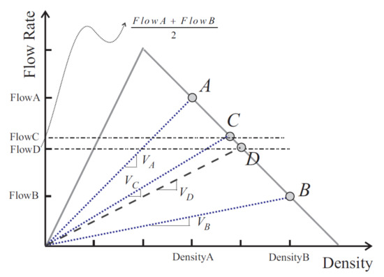
Figure 5.
Analytical speed parameter estimation.
After recognizing the average speed may not meter the intended number of vehicles, applying speed selection is investigated based on empirical analysis from VISSIM® model. Figure 6 depicts speed flow diagram obtained from VISSIM® test runs after an initialization period [35]. In each test run the desired speed of each vehicle is altered from 48 km/hr to a lower speed at simulation time 600 s with at total simulation time of 1200 s. The lower speeds simulated where 0.5 km/hr to 15 km/hr in 0.5 km/hr increment and 16 km/hr to 30 km/hr in 1 km/hr increment. Five runs were completed for each speed for a total 245 runs. Each dot in Figure 6 represents the average of flow rate and speed during a one minute interval between 660 s and 1200 s excluding transition period data between 600 s and 660 s. Figure 6 reveals that the data display a close agreement with flow and speed relationship. In the proposed model, the first 120 s estimates are excluded in aggregation right after a new speed is applied to exclude the transition period data. Based on this VISSIM® data, Table 4 is used in this study to apply on to vehicles to meter the intended traffic flow. The rollback process allows for maintaining similar traffic conditions between vehicles and transmitting accurate traffic conditions to other vehicles beyond the network boundaries of the vehicles. With proper feedback the proposed simulation will be able to capture dynamically changing traffic conditions and provide more up-to-date and more robust estimates.
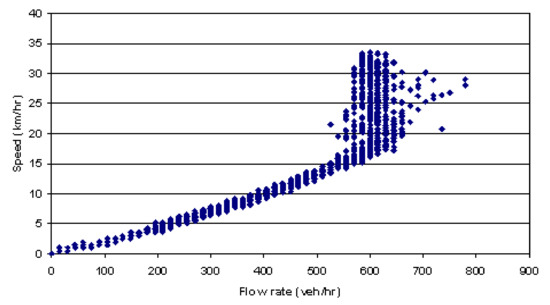
Figure 6.
Speed flow diagram.
Table 4.
Applied speed and corresponding flow rate.
6. Conclusions
In this paper, an online ad hoc distributed traffic simulation system based on optimistic execution is proposed. It is envisioned that in the proposed distributed traffic simulation framework, each in-vehicle simulation models a small portion of the overall network and provides detailed traffic state information. Traffic simulation and data processing are performed in a distributed fashion by multiple vehicles. Each in-vehicle simulation is designed to run in real-time and update its estimates when it is necessary. To handle the data received from all participating vehicles, an optimistic (rollback-based) synchronization protocol is developed. Optimistic execution inspired by Time Warp can mitigate the synchronization problem allowing each logical process to execute asynchronously. This approach provides increased computing capacity with a time-synchronized approach.
As a part of this research effort, this paper proposes an online ad hoc distributed simulation. The physical operating platform for the model including operating system, communicational middleware, and traffic simulation model are described as well as rollback process. Also, this paper investigates the analytical background of rollback process of the proposed ad hoc distributed simulation model. Flow rate diagram and cumulative number of vehicle diagram show that the overall system simulation speed and estimate accuracy may differ significantly as a function of the selected threshold. Additionally, a graphical analysis for speed selection of outflow control is presented as well as an empirical solution. The graphical method proves that applying average speed may not process the correct traffic flow.
7. Discussion
In this paper, a graphical analysis was conducted for the proposed threshold method for rollback. This rollback approach is expected to allow for maintaining similar traffic conditions between vehicles and transmitting accurate traffic conditions to other vehicles beyond the network boundaries of the vehicles. In the proposed scenarios, each in-vehicle simulation models a small portion of the overall network and provides detailed traffic state information. Traffic simulation and data processing are performed in a distributed fashion by multiple vehicles. Each in-vehicle simulation is designed to run in real-time and update its estimates when it is necessary. A local central server receives the traffic states from multiple in-vehicle simulations. Traffic estimates are not guaranteed to be received in time stamp order, since in-vehicles simulations run concurrently. Also, a traffic state can be projected by multiple in-vehicle simulations. A mechanism is needed to coordinate the transmitted data, combine values into a composite value, and save in Space-Time Memory. Optimistic execution inspired by Time Warp can mitigate the synchronization problem allowing each logical process to execute asynchronously. This approach provides increased computing capacity with a time-synchronized approach. Traffic data are constantly updated through rollbacks to reflect any traffic changes which warrant a threshold violation. The proposed methodology is aimed to provide asynchronous execution. integrate distributed traffic simulations and coordinate the estimates generated by multiple vehicles. Also, the rollback process allows for maintaining similar traffic conditions between vehicles and transmitting accurate traffic conditions to other vehicles beyond the network boundaries of the vehicles. With proper feedback the proposed simulation will be able to capture dynamically changing traffic conditions and provide more up-to-date and more robust estimates.
In a future publication, a comparison to the use of a distributed simulation standard, and a performance analysis of the simulation will be investigated. They will provide more insight regarding the applicability of the model. For the application in real world, the proposed system will have to be tested with real world data. Also, the potential market acceptance and the adoption need to be investigated. It is believed that the proposed method can function in uncongested traffic conditions. However, a more detailed analysis of the system will have to be conducted in urban environments including model validation and performance results. Robust analysis will enable researchers to better understand and apply the proposed system into large-scale transportation systems.
Funding
This work was partially supported by NRF-2020R1A2C1011060 of the Korean government.
Data Availability Statement
The data presented in this study are available on request from the corresponding author.
Acknowledgments
The author would like to acknowledge Richard Fujimoto and Michael Hunter.
Conflicts of Interest
The authors declare no conflict of interest.
References
- Henclewood, D.; Guensler, R.; Fujimoto, R.M.; Hunter, M.P.; Suh, W.; Guin, A. Real-time data-driven traffic simulation for performance measure estimation. IET Intell. Transp. Syst. 2016, 10, 562–571. [Google Scholar] [CrossRef]
- Suh, W.; Hunter, M.P.; Fujimoto, R. Ad hoc distributed simulation for transportation system monitoring and near-term prediction. Simul. Model. Pract. Theory 2014, 41, 1–14. [Google Scholar] [CrossRef]
- Suh, W.; Henclewood, D.; Guin, A.; Guensler, R.; Hunter, M.P.; Fujimoto, R. Dynamic data driven transportation systems. Multimed. Tools Appl. 2017, 76, 25253–25269. [Google Scholar] [CrossRef]
- Fujimoto, R. Parallel and Distributed Simulation Systems; Wiley-Interscience: Hoboken, NJ, USA, 2000. [Google Scholar]
- Umar, U.; Rasyid, M.U.H.A.; Sukaridhoto, S. Distributed Database Semantic Integration of Wireless Sensor Network to Access the Environmental Monitoring System. Int. J. Eng. Technol. Innov. 2018, 8, 157–172. [Google Scholar]
- Kim, S. Dual Polling Protocol for Improving Performance in Wireless Ad Hoc Networks. Int. J. Eng. Technol. Innov. 2018, 8, 1–12. [Google Scholar]
- Chang, L.-H.; Lee, T.; Chu, H.; Su, C. Application-Based Online Traffic Classification with Deep Learning Models on SDN Networks. Adv. Technol. Innov. 2020, 5, 216–229. [Google Scholar] [CrossRef]
- Fujimoto, R. Parallel and Distributed Simulation. In Proceedings of the 1999 Winter Simulation Conference, Phoenix, AZ, USA, 5–8 December 1999. [Google Scholar]
- Jefferson, D. Virtual Time. ACM Transactions on Programming Languages and Systems. 1985, Volume 7, pp. 404–425. Available online: http://cobweb.cs.uga.edu/~maria/pads/papers/p404-jefferson.pdf (accessed on 24 December 2020).
- Fujimoto, R.M. Parallel Discrete Event Simulation. In Proceedings of the 21st Conference on Winter, Washington, DC, USA, 4–6 December 1989. [Google Scholar]
- Park, A.; Fujimoto, R. A scalable framework for parallel discrete event simulations on desktop grids. In Proceedings of the 2007 8th IEEE/ACM International Conference on Grid Computing, Austin, TX, USA, 19–21 September 2007. [Google Scholar]
- Lin, Y.-B.; Fishwick, P. Asynchronous parallel discrete event simulation. IEEE Trans. Syst. Man Cybern. Part A Syst. Hum. 1996, 26, 397–412. [Google Scholar] [CrossRef]
- Lin, Y.B.; Preiss, B.; Loucks, W.; Lazowska, E. Selecting the Checkpoint Interval in Time Warp Simulation. In Proceedings of the Seventh Workshop on Parallel and Distributed Simulation, San Diego, CA, USA, 16–19 May 1993. [Google Scholar]
- Liu, H.; Ma, W.; Jayakrishnan, R.; Recker, W. Large-Scale Traffic Simulation Through Distributed Computing of Paramics; PATH Re-Search Report; UC Berkeley: California Partners for Advanced Transportation Technology: Berkeley, CA, USA, 2004. [Google Scholar]
- Nagel, K.; Cetin, N. Parallel Queue Model Approach to Traffic Microsimulations; Transportation Research Board Annual Meeting: Washington, DC, USA, 2003. [Google Scholar]
- Ben-Akiva, M.; Bierlairey, M.; Koutsopoulosz, H.; Mishalanix, R. Real Time Simulation of Traffic Demand-Supply Interactions within DynaMIT. In Transportation and Network Analysis: Current Trends; Gendreau, M., Marcotte, P., Eds.; Springer: Boston, MA, USA, 2000; Volume 63. [Google Scholar]
- Jayakrishnan, R.; Sheu, P.; Wang, T.; Xu, M. Database Environment for Fast Real-Time Simulation of Urban Traffic Networks with ATMIS; California Partners for Advanced Transit and Highways (PATH): Richmond, CA, USA, 2000. [Google Scholar]
- Yang, Q.; Koutsopoulos, H.N. A Microscopic Traffic Simulator for evaluation of dynamic traffic management systems. Transp. Res. Part C Emerg. Technol. 1996, 4, 113–129. [Google Scholar] [CrossRef]
- Nagel, K.; Rickert, M. Parallel implementation of the TRANSIMS micro-simulation. Parallel Comput. 2001, 27, 1611–1639. [Google Scholar] [CrossRef]
- Rickert, M.; Nagel, K. Dynamic traffic assignment on parallel computers in TRANSIMS. Future Gener. Comput. Syst. 2001, 17, 637–648. [Google Scholar] [CrossRef]
- Gu, Y. Integrating a Regional Planning Model (TRANSIMS) With an Operational Model (CORSIM). In Civil Engineering; Virginia Polytechnic Institute and State University: Blacksburg, VA, USA, 2004. [Google Scholar]
- Barceló, J.; Ferrer, J.; García, D.; Grau, R. Microscopic Traffic Simulation for ATT Systems Analysis—A Parallel Computing Version. In Equilibrium and Advanced Transportation Modelling. Centre for Research on Transportation; Marcotte, P., Nguyen, S., Eds.; Springer: Boston, MA, USA, 1998. [Google Scholar]
- Algers, S.; Bernauer, E.; Boero, M.; Breheret, L.; Taranto, C.; Dougherty, M.; Fox, K.; Gabard, J. Review of Micro-Simulation Models. 1997. Available online: https://www.semanticscholar.org/paper/Review-of-MicroSimulation-Models-Algers-Bernauer/f981a04dbf276f4298bdaab3b5acf43af6fcea5f (accessed on 24 December 2020).
- Cameron, G.; Wylie, B.J.N.; McArthur, D. PARAMICS-moving vehicles on the connection machine. In Proceedings of the 1994 ACM/IEEE Conference on Supercomputing—Supercomputing ’94, Washington, DC, USA, 14–18 November 2002. [Google Scholar]
- Cameron, D.; Duncan, G. PARAMICS—Parallel Microscopic Simulation of Road Traffic. J. Supercomput. 1996, 10, 25–53. [Google Scholar] [CrossRef]
- Lee, D.H.; Chandrasekar, P. A Framework for Parallel Traffic Simulation Using Multiple Instancing of a Simulation Program. Intell. Transp. Syst. J. 2004, 7, 279–294. [Google Scholar] [CrossRef]
- Klefstad, R.; Zhang, Y.; Lai, M.; Jayakrishnan, R.; Lavanya, R. A distributed, scalable, and synchronized framework for large-scale mi-croscopic traffic simulation. In Proceedings of the IEEE Conference on Intelligent Transportation Systems, Vienna, Austria, 13–16 September 2005. [Google Scholar]
- Bononi, L.; Di Felice, M.; D’Angelo, G.; Bracuto, M.; Donatiello, L. MoVES: A framework for parallel and distributed simulation of wireless vehicular ad hoc networks. Comput. Netw. 2008, 52, 155–179. [Google Scholar] [CrossRef]
- Sippl, C.; Schwab, B.; Kielar, P.M.; Djanatliev, A. Distributed Real-Time Traffic Simulation for Autonomous Vehicle Testing in Urban Environments. In Proceedings of the 2018 21st International Conference on Intelligent Transportation Systems (ITSC), Maui, HI, USA, 4–7 November 2018. [Google Scholar]
- Mastio, M.; Zargayouna, M.; Scemama, G.; Rana, O. Distributed Agent-Based Traffic Simulations. IEEE Intell. Transp. Syst. Mag. 2018, 10, 145–156. [Google Scholar] [CrossRef]
- Raghothama, J.; Meijer, S. Distributed, integrated and interactive traffic simulations. In Proceedings of the 2015 Winter Simulation Conference (WSC), Huntington Beach, CA, USA, 6–9 December 2015; pp. 1693–1704. [Google Scholar]
- Chan, C.; Wang, B.; Bachan, J.; Macfarlane, J. Mobiliti: Scalable Transportation Simulation Using High-Performance Parallel Computing. In Proceedings of the 2018 21st International Conference on Intelligent Transportation Systems (ITSC), Maui, HI, USA, 4–7 November 2018; pp. 634–641. [Google Scholar]
- Suh, W.; Park, J.W.; Kim, J.R. Traffic Safety Evaluation Based on Vision and Signal Timing Data. Proc. Eng. Technol. Innov. 2017, 7, 37–40. [Google Scholar]
- Suh, W.; Kim, J.R.; Cho, J. Vision Technology Based Traffic Safety Analysis Using Signal Data. Proc. Eng. Technol. Innov. 2019, 13, 20–25. [Google Scholar]
- Suh, W. Mitigating Initialization Bias in Transportation Modeling Applications. Proc. Eng. Technol. Innov. 2016, 3, 34–36. [Google Scholar]
Publisher’s Note: MDPI stays neutral with regard to jurisdictional claims in published maps and institutional affiliations. |
© 2020 by the author. Licensee MDPI, Basel, Switzerland. This article is an open access article distributed under the terms and conditions of the Creative Commons Attribution (CC BY) license (http://creativecommons.org/licenses/by/4.0/).