Article

Application of Improved LightGBM Model in Blood Glucose Prediction

School of Computer and Communication, Lanzhou University of Technology, Lanzhou 730050, China
*
Author to whom correspondence should be addressed.
Appl. Sci. 2020, 10(9), 3227; https://doi.org/10.3390/app10093227
Submission received: 6 April 2020 / Revised: 28 April 2020 / Accepted: 2 May 2020 / Published: 6 May 2020
(This article belongs to the Section Applied Biosciences and Bioengineering)

Abstract

:
In recent years, with increasing social pressure and irregular schedules, many people have developed unhealthy eating habits, which has resulted in an increasing number of patients with diabetes, a disease that cannot be cured under the current medical conditions, and can only be mitigated by early detection and prevention. A lot of human and material resources are required for the detection of the blood glucose of a large number of people in medical examination, while the integrated learning model based on machine learning can quickly predict the blood glucose level and assist doctors in treatment. Therefore, an improved LightGBM model based on the Bayesian hyper-parameter optimization algorithm is proposed for the prediction of blood glucose, namely HY_LightGBM, which optimizes parameters using a Bayesian hyper-parameter optimization algorithm based on LightGBM. The Bayesian hyper-parameter optimization algorithm is a model-based method for finding the minimum value of the function so as to obtain the optimal parameters of the LightGBM model. Experiments have demonstrated that the parameters obtained by the Bayesian hyper-parameter optimization algorithm are superior to those obtained by a genetic algorithm and random search. The improved LightGBM model based on the Bayesian hyper-parameter optimization algorithm achieves a mean square error of 0.5961 in blood glucose prediction, with a higher accuracy than the XGBoost model and CatBoost model.

1. Introduction

The recent years have seen a rapid increase in the incidence of diabetes around the world, due to many factors such as the continuous improvement in people’s living standards, changes in dietary structure, an increasingly rapid pace of life, and a sedentary lifestyle. Diabetes has become the third major chronic disease that seriously threatens human health, following cancer and cardiovascular disease [1,2]. According to statistics from the International Diabetes Federation (IDF), there were approximately 425 million patients with diabetes across the world in 2017. One in every 11 adults has diabetes, and one in every two patients is undiagnosed [3]. As of 2016, diabetes directly caused 1.6 million deaths [4], and it is estimated that by 2045, nearly 700 million people worldwide will suffer from diabetes, which will pose an increasing economic burden on health systems in most of countries. It is forecast that by 2030, at least $490 billion will be spent on diabetes globally [5].
Currently, the diagnosis rate of diabetes is low, as patients exhibit no obvious symptoms in the early onset of the disease, and many people do not realize they have the disease [6]; thus, early detection and diagnosis are particularly needed. It is relatively simple to measure a person’s blood glucose under the existing medical conditions, but it takes a lot of human and material resources to detect the blood glucose of a large number of people in medical examination. Therefore, the prediction of the blood glucose of a large number of people in medical examination by machine learning can save a lot of unnecessary expenses (for example [7]).
With the application of machine learning in medical fields, more and more people are applying emerging prediction methods to many different medical fields to help greatly reduce the workload of the related medical staff and improve the diagnosis efficiency of doctors. For example, Yu Daping and Liu applied the XGBoost model for the early diagnosis of lung cancer [8]. Tjeng Wawan Cenggoro used the XGBoost model to predict and analyze colorectal cancer in Indonesia [9]. Chang Wenbing forecasted the prognosis of hypertension using the XGBoost model [10]. Ogunleye Adeola Azeez applied the XGBoost model for the diagnosis of chronic kidney disease [11]. Wenbing Chang used the XGBoost model and clustering algorithm to analyze the probability of hypertension-related symptoms [12]. Wang Bin predicted severe hand, foot, and mouth disease using the CatBoost model [13].
As the XGBoost model generates a decision tree using the level-wise method [14], it the splits leaves simultaneously on the same layer, but the splitting gain of most leaf nodes is low. In many cases where further splitting is unnecessary, the XGBoost model will continue to split, causing non-essential expenses. Compared with the LightGBM model, the XGBoost model occupies more memory and consumes more time when the dataset is large.
The traditional genetic algorithm and random search algorithm have different defects—the genetic algorithm is a natural adaptive optimization method that simulates the problem to be solved as a process of biological evolution, and gradually eliminates the solutions with low fitness function values through generating next-generation solutions by operations such as replication, crossover, and mutation [15]. The genetic algorithm uses the search information of multiple search points at the same time, and adopts probabilistic search technology to obtain the optimal or sub-optimal solution of the optimization problem. It boasts of good search flexibility, global search capability, and is easily implemented [16]. However, it has a poor local search ability, complicated process caused by many control variables, and there are no definite termination rules. The random searching algorithm (RandomizedSearchCV) performs a random search in a set parameter search space. It samples a fixed number of parameters from a specified distribution instead of trying all of the parameter values [17]. However, the random searching algorithm exhibits a poor performance when the dataset is small. Therefore, this paper proposes an improved LightGBM model for blood glucose prediction.
The main contributions of this study are as follows: by preprocessing the data on various medical examination indicators of people receiving medical examination, this paper proposes a LightGBM model optimized by the Bayesian hyper-parameter optimization algorithm to predict the blood glucose level of people receiving medical examination. The LightGBM model optimized by the Bayesian hyper-parameter optimization algorithm achieves a higher accuracy than the XGBoost model, Catboost model, the LightGBM model optimized by genetic algorithm, and the LightGBM model optimized by random searching algorithm, which can help doctors give early warning to those potentially suffering from diabetes, so as to reduce the incidence of diabetes, increase the diagnosis rate, and provide new ideas for the in-depth study on diabetes. The proposed method was verified by the diabetes data from a grade-three first-class hospital in China from September to October 2017.

2. Materials and Methods

2.1. LightGBM Model

LightGBM is an improvement framework based on decision tree algorithm released by Microsoft in 2017. LightGBM and XGBoost both support parallel arithmetic, but LightGBM is more powerful than the previous XGBoost model, with a fast training speed and less memory occupation, which can reduce the communication cost of parallel learning. LightGBM is mainly featured by the decision tree algorithm based on gradient-based one-side sampling (GOSS), exclusive feature bundling (EFB), and a histogram and leaf-wise growth strategy with a depth limit.
The basic idea of GOSS (gradient-based one-side sampling) is to keep all of the large gradient samples and to perform random sampling on the small gradient samples according to proportion. The basic idea of the EFB (exclusive feature bundling) algorithm is to divide the features into a smaller number of mutually exclusive bundles, that is, it is impossible to find an accurate solution in polynomial time. Therefore, what it uses is an approximate solution, that is, a small number of sample points that are not mutually exclusive are allowed between features (for example, some corresponding sample points are not non-zero at the same time). Allowing a small part of conflict can obtain a smaller number of feature bundles, which further improves the computational effectiveness [18].
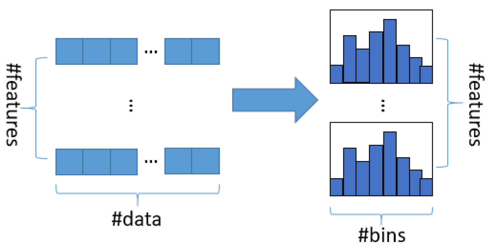
The basic idea of the histogram algorithm is to discretize continuous floating point features into k integers, and to construct a histogram with a width of k at the same time. When the data are traversed, statistics is accumulated in the histogram with the discretized value as index. After the data are traversed once, the histogram accumulates the required volume of statistics, and then the optimal segmentation point can be found through traverse according to the discrete value in the histogram, as shown in Figure 1:
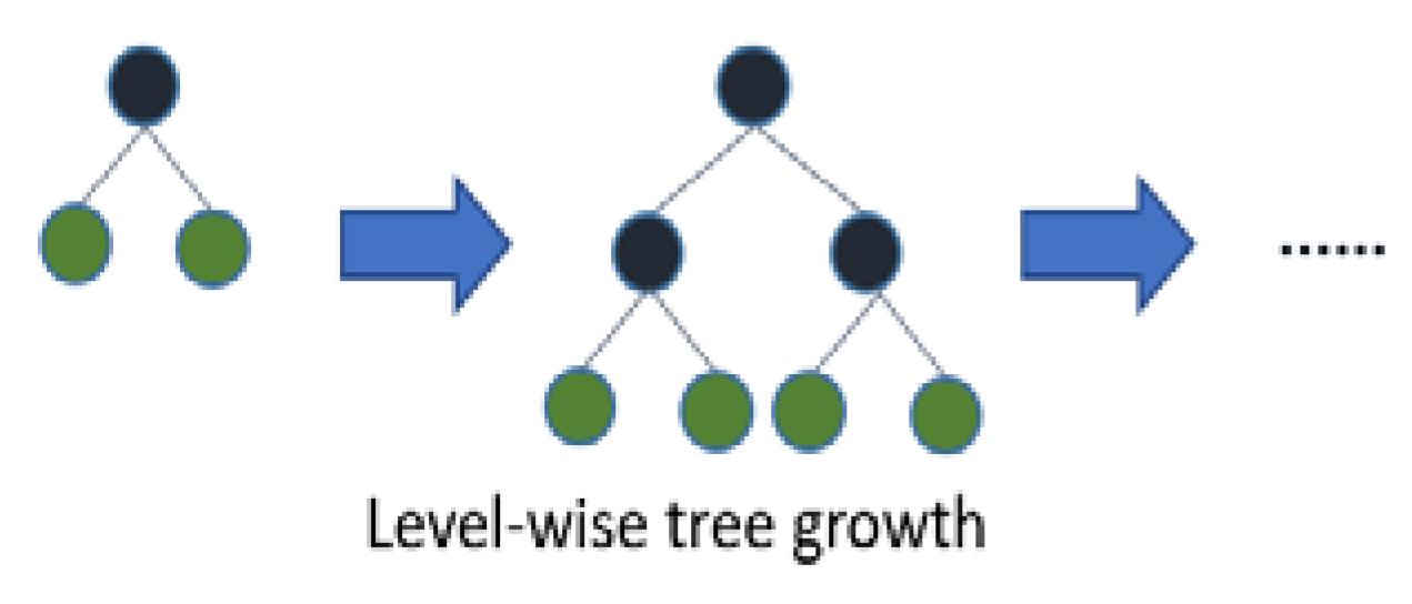
Most of the learning algorithm tree of decision tree is generated by the level-wise growth method, such as XGBoost, as shown in Figure 2:
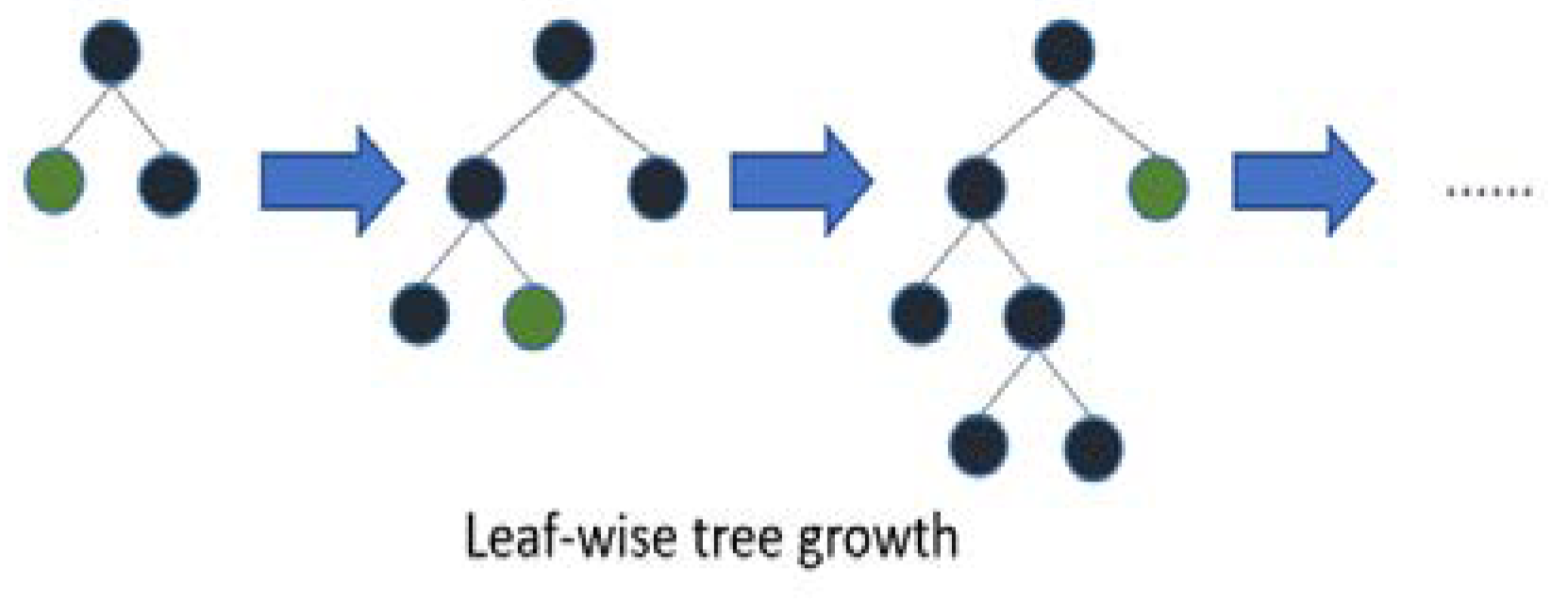
LightGBM uses a leaf-wise growth strategy with a depth limit to find a leaf node with the largest split gain in all of the current leaf nodes, then splits, and so on, as shown in Figure 3:
Compared with the level-wise growth strategy, leaf-wise tree growth can reduce large errors and achieve a higher accuracy, thereby providing solutions to many problems. For example, Xile Gao used Stacked Denoising Auto Encoder (SDAE) and LightGBM models to recognize human activity [19]; Sunghyeon Choi employed a random forest, XGBoost model, and LightGBM model to predict solar energy output [20]; João Rala Cordeiro forecasted children’s height using a XGBoost model and LightGBM model [21]; Ma Xiaojun et al. adopted a LightGBM model and XGBoost model to predict the default of P2P network loans [22]; Chen Cheng et al. used LightGBM and a multi-information fusion model to predict the interaction between proteins [23]; and Vikrant A. Dev applied a LightGBM model to stratum lithology classification [24].
The following is the introduction to the theory of the LightGBM model’s objective function: yi is the objective value, i is the predicted value, T represents the number of leaf nodes, q denotes the structure function of the tree, and w is the leaf weight.
The objective function is as follows:
O bj ( t ) = i = 1 n l ( y i , y ^ i ( t ) ) + i = 1 t Ω ( f i ) = i = 1 n l ( y i , y ^ i ( t 1 ) + f t ( x i ) ) + i = 1 t Ω ( f i )
Logistic loss:
L ( θ ) = i [ y i ln ( 1 + e y ^ i ) + ( 1 y i ) ln ( 1 + e ) y ^ i ]
Use the Taylor expansion to define the objective function:
f ( x + Δ x ) f ( x ) + f ( x ) Δ x + 1 2 f ( x ) Δ x 2
At this time, the objective function is the following:
O b j ( t ) = i = 1 n [ l ( y i , y ^ ( t 1 ) ) + g i f t ( x i ) + 1 2 h i f t 2 ( x i ) ] + Ω ( f t )
Among:
g i = y ^ i ( t 1 ) l ( y i , y ^ ( t 1 ) ) , h i = y ^ i ( t 1 ) 2 l ( y i , y ^ ( t 1 ) )
Use the accumulation of n samples to traverse all of the leaf nodes:
O b j ( t ) i = 1 n [ g i f t ( x i ) + 1 2 h i f t 2 ( x i ) ] + Ω ( f ( t ) )
where Ij is the sample set in leaf node j, namely:
G j = i I j g i , H j = i I j h i
Therefore:
O b j ( t ) = j = 1 T [ ( i I j g i ) w j + 1 2 ( i I i h j + λ ) w j 2 ] = j = 1 T [ G j w j + 1 2 ( H j + λ ) w j 2 ]
The partial derivative of the output Wj of the jth leaf node is obtained, and the minimum value is obtained as follows:
w j [ ( i I j g i ) w j + 1 2 ( i I j h i + λ ) w j 2 ] = i I j g i + ( i I j h i + λ ) w j
Solution:
w j = G j H j + λ
When the structure of the q (x) tree is determined, the function Lt(q) is obtained, as follows:
L t ( q ) = j = 1 T G j w j + 1 2 ( H j + λ ) w j 2 = j = 1 T [ G j ( G j H j + λ ) + 1 2 ( H j + λ ) ( G j H j + λ ) 2 ] = j = 1 T G j 2 H j + λ + 1 2 G j 2 H j + λ = 1 2 j = 1 T G j 2 H j + λ
The calculated gain is the following:
G = 1 2 [ G L 2 H L + λ + G R 2 H R + λ ( G L + G R ) 2 H L + H R + λ ]

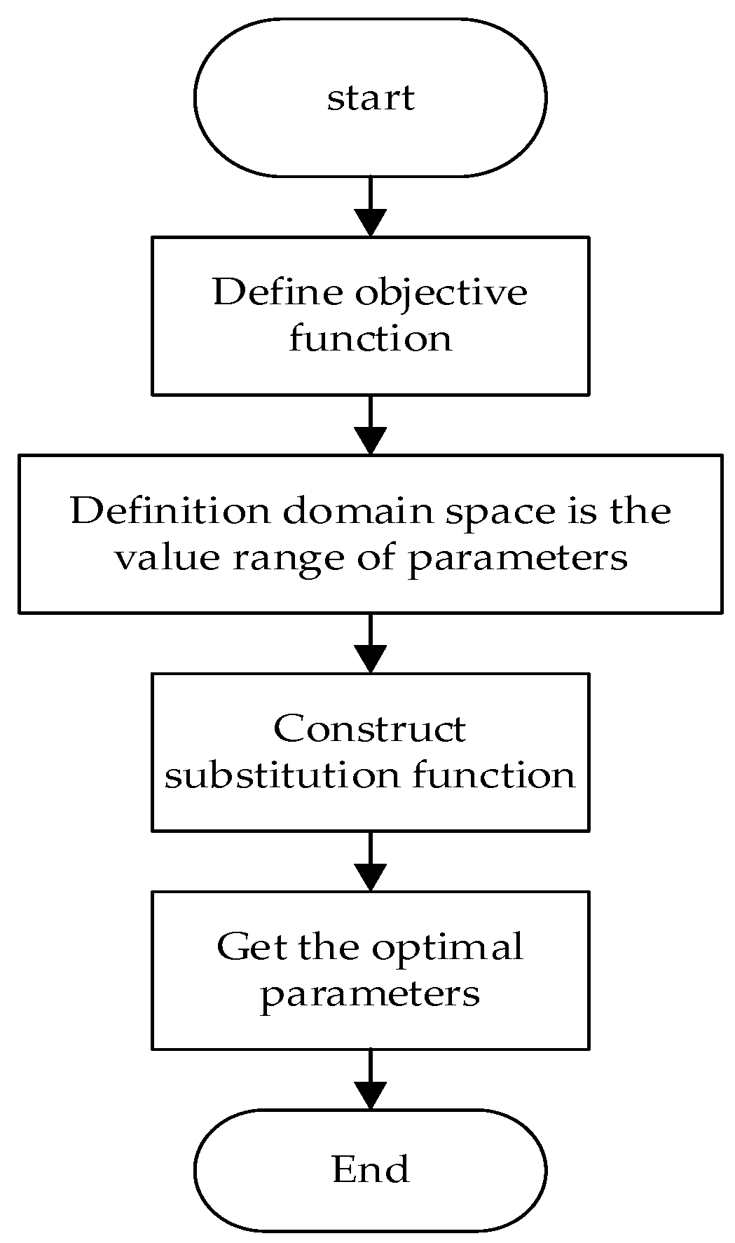
2.2. Bayesian Hyper-Parameter Optimization Algorithm

The basic idea of the Bayesian hyper-parameter optimization algorithm is to establish a substitute function based on the evaluation result of the past objective to find the minimum value of the objective function. The substitute function established in this process is easier to optimize than the original objective function, and the input value to be evaluated is selected by applying a certain standard to the proxy function [25]. Although the genetic algorithm is currently widely used in the parameter optimization of machine learning [26,27,28,29], its disadvantages are also obvious, such as a poor ability of local search, many control variables, a complicated process, and no determined termination rules. The random searching algorithm is a traditional parameter optimization algorithm in machine learning [30]. It uses random sampling within the search range for parameter optimization, but the effect is poor when the dataset is small. In contrast, Bayesian hyper-parameter optimization takes the result of the previous evaluation into account when trying another set of hyper-parameters, and has a simpler process of optimizing model parameters than the genetic algorithm, which can save a lot of time.
The HY_LightGBM model proposed in this paper uses one of the Bayesian optimization libraries in Python, Hyperopt, which uses Tree Parzen Estimation (TPE) as the optimization algorithm.
The optimization process of the Bayesian optimization algorithm is shown in Figure 4.
By defining the objective function, domain space, and constructing the substitution function, the optimal parameters were finally obtained, with mean square error (MSE) as the evaluation indicator. The obtained optimal parameters were input into the LightGBM model to further improve the prediction ability of the model.

2.3. Improved LightGBM Model Based on Bayesian Hyper-Parameter Optimization Algorithm

The experiment was conducted on a computer with Intel I5 8400 2.8 GHz six-core six-thread central processing unit (CPU), 16G random-access memory (RAM), and Windows 10 operating system. The simulation platform is Pycharm, and Python was used for programming, with sklearn, pandas, and numpy libraries adopted.
Because LightGBM has many parameters, the manual adjustment of parameters will be complicated, and considering its parameters have a great impact on experimental results, it is particularly necessary to use Bayesian hyper-parameter optimization algorithm for parameter optimization. The Hyperopt used in this paper is one of the Bayesian optimization libraries in Python. It is also a class library used in distributed asynchronous algorithm configuration in Python, with a faster speed and better effect in finding the optimal parameters of the model than the traditional parameter optimization algorithms.
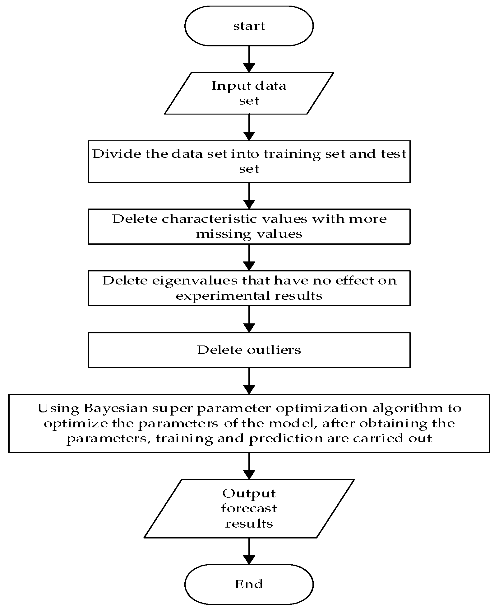
The specific steps are as follows:
(1)
Divide the dataset into training set and test set, process the missing values, analyze the weight of the influence of the eigenvalues on the results, delete useless eigenvalues, and delete outliers;
(2)
Use the Bayesian hyper-parameter optimization algorithm for the parameter optimization of the LightGBM model, and the HY_LightGBM model is constructed and trained;
(3)
Use the HY_LightGBM model for prediction and output the prediction results.
(4)
The specific experimental process is shown in Figure 5.

2.4. Data Preprocessing

The dataset in this paper is the diabetes data from September to October 2017 in a grade-three first-class hospital, provided by the Tianchi competition platform as the data source, with a total of 7642 pieces of data and 42 eigenvalues, As shown in Table 1. The eigenvalues include the following:
In this paper, the dataset was divided, with 6642 pieces of data as the training set, and the remaining 1000 pieces of data as the test set.
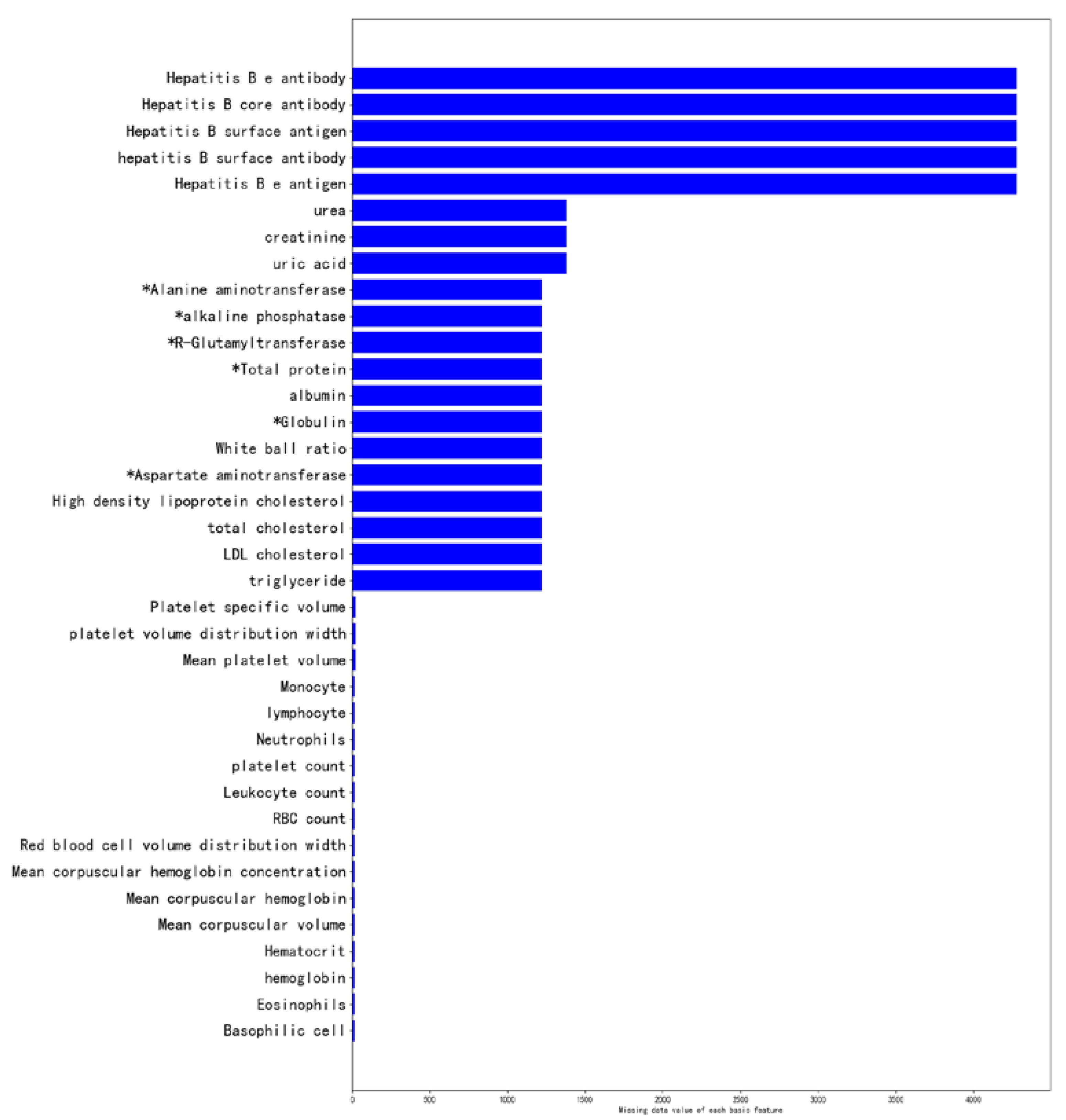
Firstly, the missing values in the original dataset were analyzed to obtain the proportion of the missing data. It can be seen from Figure 6 that the missing proportion of five basic features—hepatitis B surface antigen, hepatitis B surface antibody, hepatitis B core antibody, hepatitis B e antigen, and hepatitis B e antibody—is over 70%, significantly exceeding the missing proportion of other basic features. Therefore, these features with large missing values were deleted, and those with smaller missing values were filled with medians.
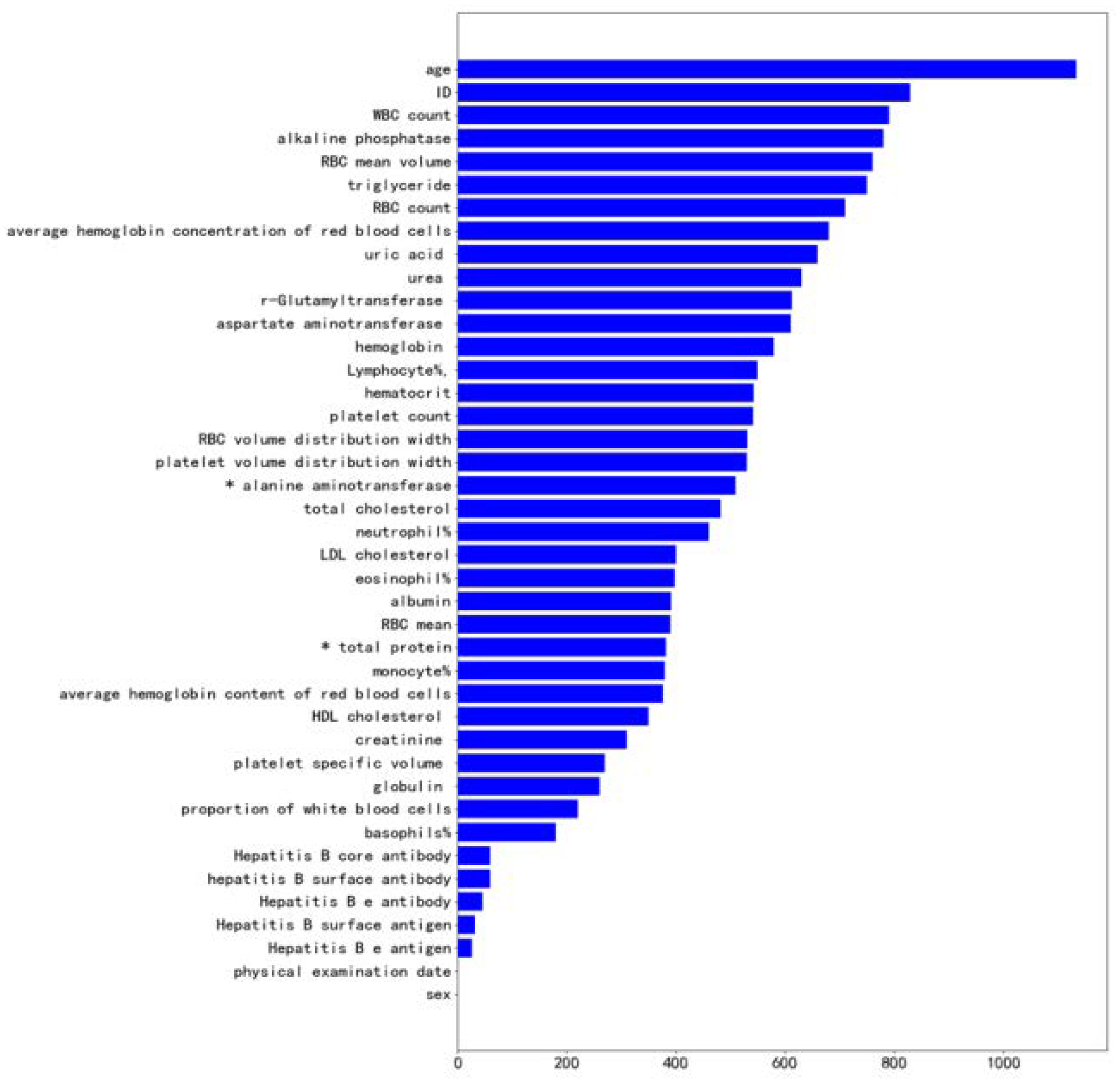
Secondly, the weight of the influence of the data features was analyzed. The weight of the eigenvalues can be obtained through related functions. According to the eigenvalue weight of each item, the eigenvalues that have no effect on the results can be found. By processing the invalid eigenvalues, the accuracy of the experiment can be further improved. It can be seen from Figure 7 that the date of medical examination and gender have no practical influence on the prediction results of the model. It can be known through common sense that ID also has no impact on the experimental results, so these features were deleted.
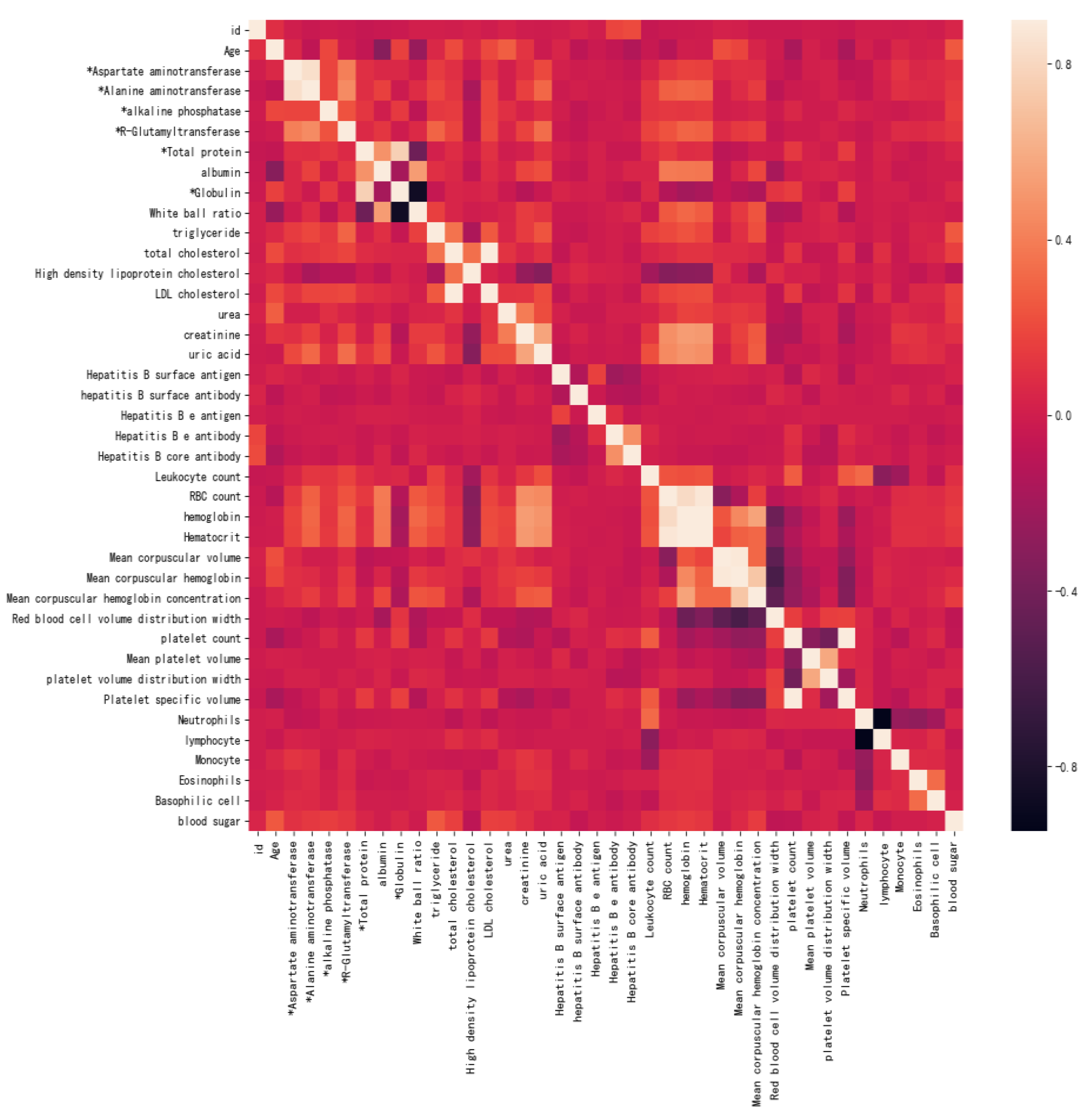
Again, to analyze the correlation coefficient of each eigenvalue, the darker the color, the stronger the correlation. From Figure 8, we can see the correlation between each eigenvalue.
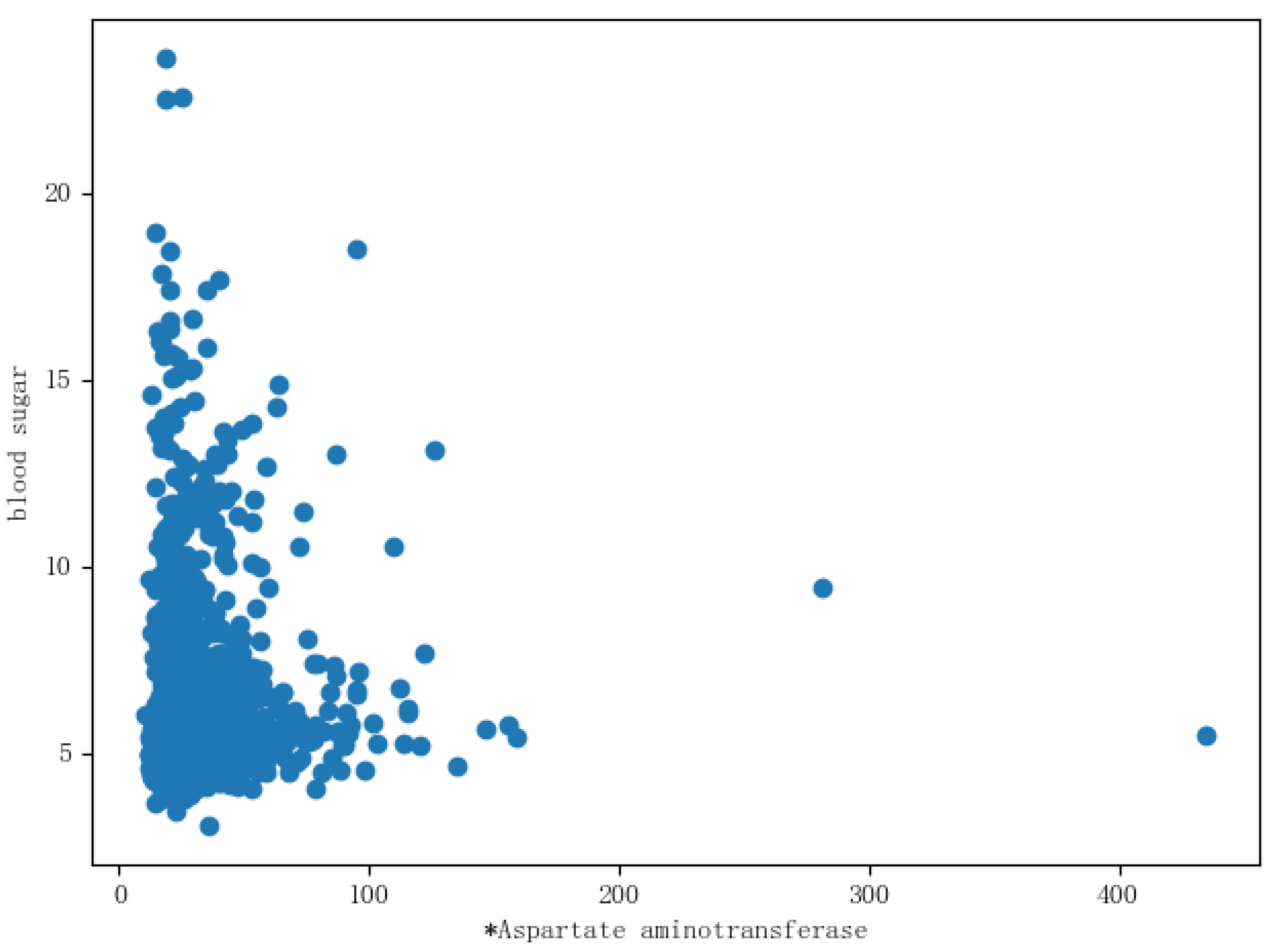
Finally, the basic features and the distribution of the blood glucose levels were learned, which can provide a more intuitive reference for feature engineering. The blood glucose values were used as the Y-axis coordinates and the other basic features as the X-axis coordinates. Each basic feature and the distribution of the blood glucose value were listed for analysis, as shown in Figure 9, where aspartate aminotransferase and the distribution of blood glucose are displayed. It can be seen from the figure that the distribution of the blood glucose value in aspartate aminotransferase included outliers, so the outliers were deleted. The outliers of the remaining features were also deleted.

2.5. Parameter Optimization Based on Bayesian Hyper-Parameter Optimization Algorithm

The optimal parameters of the LightGBM model were found by the Bayesian hyper-parameter optimization algorithm. Firstly, Hyperopt’s own function was used to define the parameter space, then the model and score acquirer were created, and finally, MSE was used as the evaluation indicator to obtain the optimal parameters of the LightGBM model. The optimal parameters of the LightGBM model obtained through the Bayesian hyper-parameter optimization algorithm are shown in Table 2.

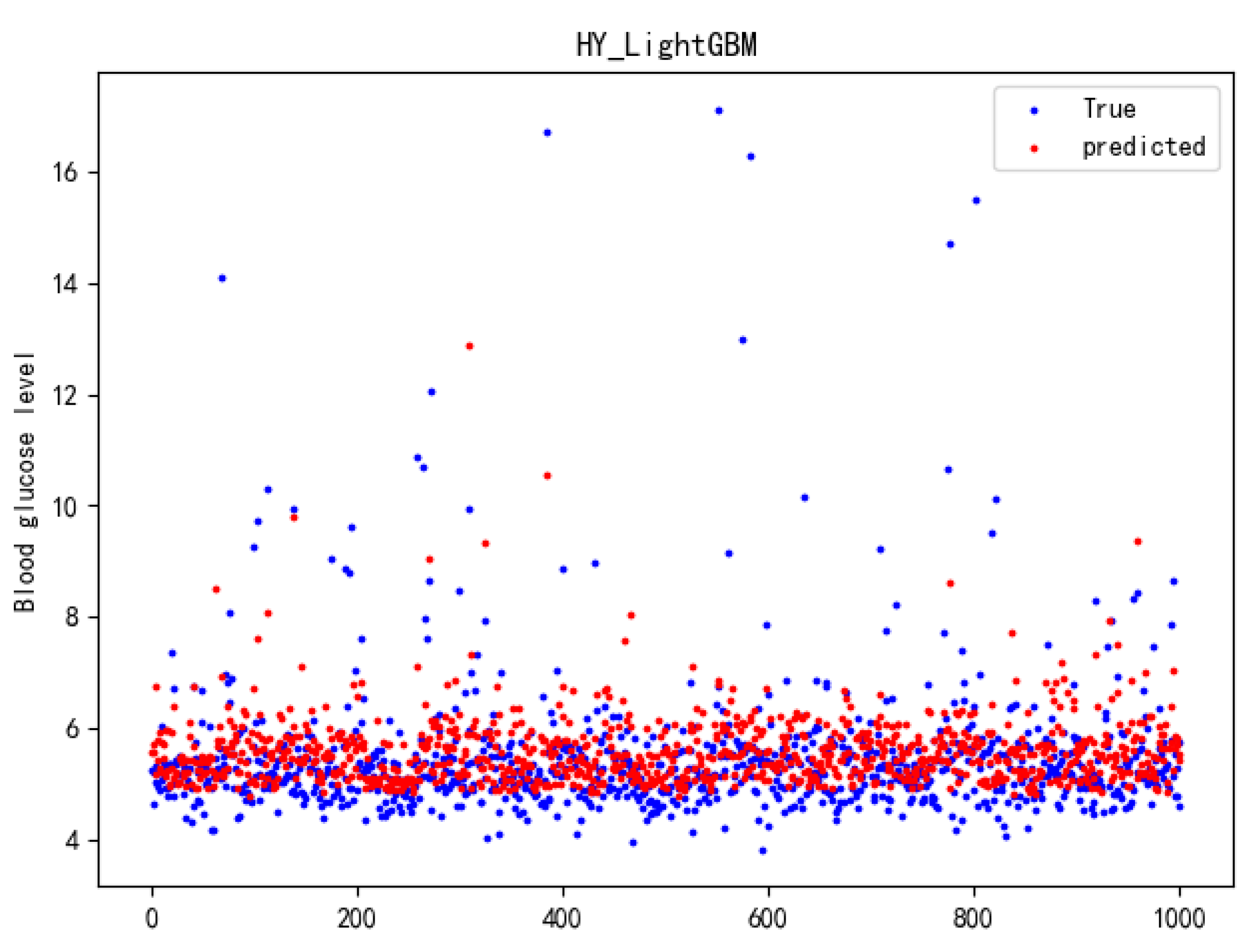
2.6. Blood Glucose Prediction by HY_LightGBM Model

Through the data preprocessing in Section 2.4 and Section 2.5 and the Bayesian hyper-parameter optimization algorithm, the optimal parameters of the LightGBM model were determined and input into the LightGBM model for training and prediction. The blood glucose values output by it and the blood glucose values in the test set were evaluated by three evaluation indicators, namely: mean square error (MSE), root mean square error (RMSE), and determination coefficient R2 (R-Square).

2.7. Evaluation Indicators

The performance of the blood glucose prediction model was evaluated by the following three indicators: mean square error (MSE), root mean square error (RMSE), and determination coefficient R2 (R-Square). These are commonly used in regression tasks, and the smaller the mean square error (MSE) and the root mean square error (RMSE) value, the more accurate the prediction results.
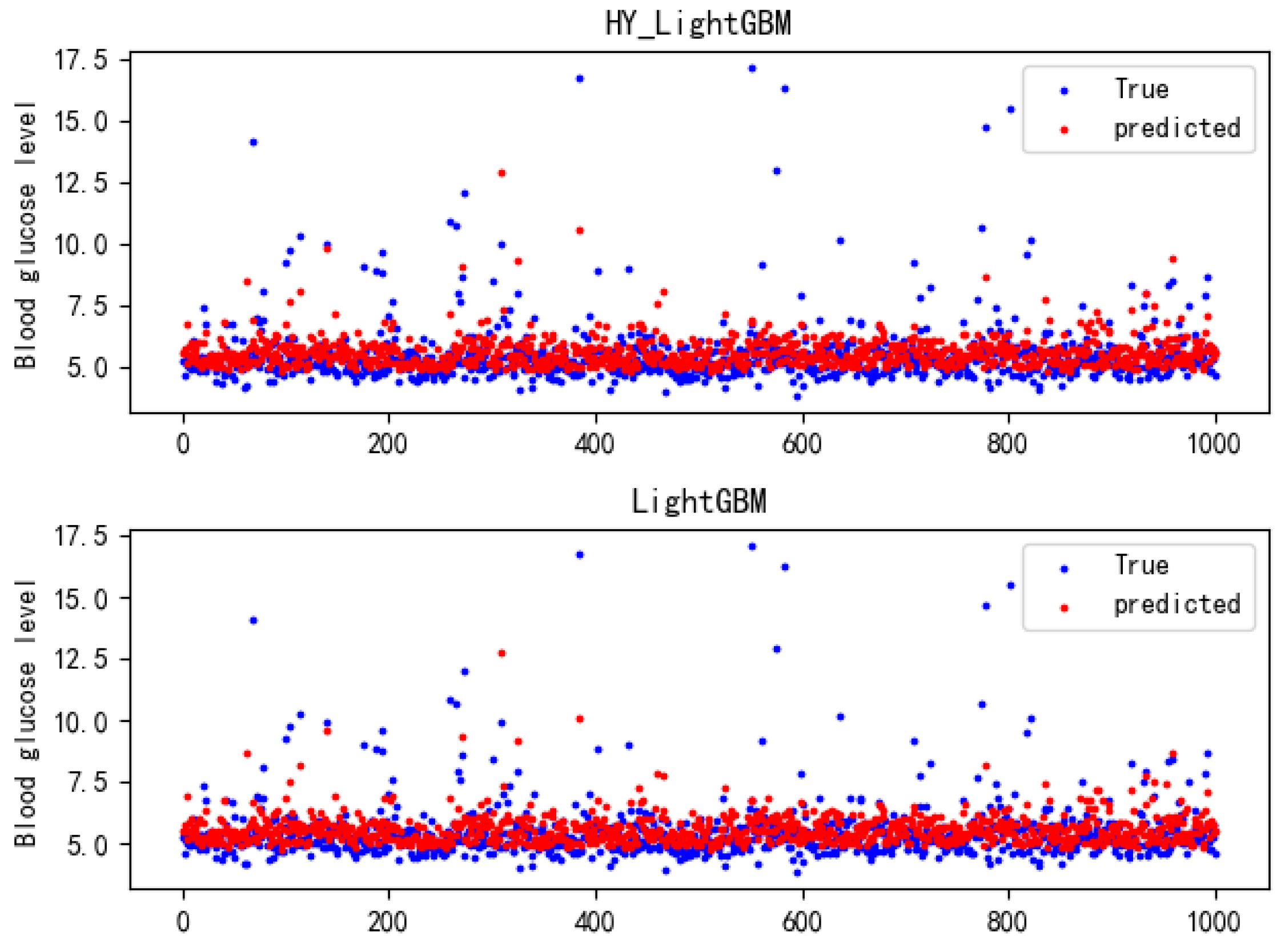
M S E = 1 2 n i = 1 n ( y i y ^ i ) 2
R M S E = 1 2 n i = 1 n ( y i y ^ i ) 2
R squaed = 1 i = 1 n ( y i y ^ i ) 2 i = 1 n ( y i y i ) 2

3. Experimental Results and Discussion

3.1. Experimental Results

After the parameter optimization of the LightGBM model by the Bayesian hyper-parameter optimization algorithm, the parameters of the LightGBM model obtained were set as follows: the learning_rate was 0.052 and the number of basic learners n_estimators was 376. The minimum row tree that the leaf may have, the tree min_data_in_leaf, is 18. The ratio of data used in each iteration bagging_fraction was 0.9, and the ratio of randomly selected features in each iteration feature_fraction was 0.5. This set of optimal parameters of the LightGBM models were input into the LightGBM model to predict the blood glucose value. The experimental results are shown in Table 3. The scatter diagram of the actual blood glucose values and the predicted blood glucose values is shown in Figure 10.
It can be found from Table 3 that the HY_LightGBM model had a mean square error of 0.5961, a root mean square error of 0.7721, a determination coefficient of 0.2236, and a training time of 26.7938 s in the prediction of the blood glucose values.

3.2. Comparative Experiments

Two groups of comparative experiments were set in the study. The first group of comparative experiments was as follows: comparing the HY_LightGBM model optimized by the Bayesian hyper-parameter optimization algorithm with the LightGBM model, the XGBoost model, and the CatBoost model without parameter optimization. The second group of the comparative experiments was as follows: the comparison among the LightGBM model with parameter optimization by genetic algorithm, the LightGBM model with parameter optimization through random searching algorithm, and the LightGBM model with parameter optimization by the Bayesian hyper-parameter optimization algorithm used in this study. The comparative experiments verified the improvement in the prediction accuracy of the HY_LightGBM model optimized by the Bayesian hyper-parameter optimization algorithm and the feasibility of the HY_LightGBM model.

3.2.1. Comparison between the HY_LightGBM Model and LightGBM Model

This experiment verified the effectiveness of the Bayesian hyper-parameter optimization algorithm for improving the LightGBM model by comparing the LightGBM model optimized by the Bayesian hyper-parameter optimization algorithm with the LightGBM model without parameter optimization. The optimal parameters found by the Bayesian hyper-parameter optimization algorithm were input into the LightGBM model, and the prediction result of the improved HY_LightGBM model was compared with that of the LightGBM model. The specific experimental results are shown in Table 4 and Figure 11.
The experiment demonstrated that although the LightGBM model optimized by the Bayesian hyper-parameter optimization algorithm takes a little more time than the LightGBM model without parameter optimization, it significantly outperforms the LightGBM model without any parameter optimization in terms of prediction accuracy.

3.2.2. Comparison between HY_LightGBM Model and Other Classification Models

In order to further verify the prediction performance of the HY_LightGBM model, two other models of the same type were selected for comparison, namely the XBGoost model and the CatBoost model. The experiment confirmed that the HY_LightGBM model has a significantly higher prediction accuracy than the other two models of the same type. The experimental results are shown in Table 5 and Figure 12.
The experiment proved that the LightGBM model optimized by the Bayesian hyper-parameter optimization algorithm used in this paper is significantly superior to the XGBoost model and CatBoost model in prediction accuracy.

3.2.3. Comparison of Parameter Tuning among Bayesian Hyper-Parameter Optimization Algorithm, Genetic Algorithm, and Random Searching Algorithm

This experiment verified the feasibility of the Bayesian hyper-parameter optimization algorithm for parameter optimization by comparing the performance of genetic algorithm, random searching algorithm, and the Bayesian hyper-parameter optimization algorithm in the parameter optimization. The parameters obtained by genetic algorithm were as follows: learning_rate was 0.05, the number of basic learners n_estimators was 400, the minimum row tree that the leaf may have min_data_in_leaf 60, the data ratio used in each iteration bagging_fraction 0.9, and the ratio of randomly selected features in each iteration feature_fraction 0.5.
The parameters obtained by the random searching algorithm were as follows: learning_rate 0.05, the number of basic learners n_estimators 370, the minimum row tree that the leaf may have min_data_in_leaf 36, the data ratio used in each iteration bagging_fraction 0.9, and the ratio of randomly selected features in each iteration feature_fraction 0.98, as shown in Table 6.
The prediction results obtained by the LightGBM model optimized by the genetic algorithm and random searching algorithm, that is, the GA_LightGBM and RS_LightGBM model, were compared with those of the LightGBM model optimized by the Bayesian hyper-parameter optimization algorithm, and the comparison results are shown in Table 7 and Figure 13 respectively.
The experiment demonstrated that the LightGBM model optimized by the Bayesian hyper-parameter optimization algorithm achieves significantly better prediction results than the LightGBM model optimized by the genetic algorithm and random searching algorithm.

4. Conclusions

This paper proposes an improved LightGBM prediction model based on the Bayesian hyper-parameter optimization algorithm, namely the HY_LightGBM model, where Bayesian hyper-parameter optimization was employed to find the optimal parameter combination for the model, which improved the prediction accuracy of the LightGBM model. The experiments proved that the method proposed in this paper achieves a higher prediction accuracy than the XGBoost model and CatBoost model, and has higher efficiency than the genetic algorithm and random searching algorithm.
The previous measurement of the blood glucose value needs to measure each person’s blood glucose value one by one, which requires a lot of manpower and material resources. After training, the model will no longer need the characteristic value of the blood glucose value. It can directly predict the blood glucose value of the physical examination personnel through the HY_LightGBM model and other physical examination indicators of the physical examination personnel.
The HY_LightGBM model, with a strong generalization ability, can also be applied to other types of auxiliary diagnosis and treatment, but the overall performance can be further improved. The next work will focus on the further optimization of the model using the idea of model fusion to improve the prediction accuracy of the model.

Author Contributions

Conceptualization, T.W.; methodology, T.W.; software, T.W.; validation, T.W.; formal analysis T.W.; investigation, T.W.; resources, T.W.; writing (original draft preparation), T.W.; writing (review and editing), T.W., Y.W.; visualization, T.W.; supervision, T.W.; project administration, T.W.; funding acquisition, Y.W. All authors have read and agree to the published version of the manuscript.

Funding

This research is supported by the key R & D plan of Gansu Province (18YF1GA060).

Conflicts of Interest

The authors declare no conflict of interest.

References

  1. American Diabetes Association. Standards of Medical Care in Diabetes—2019. Diabetes Care 2019, 42, S1–S2. [Google Scholar] [CrossRef] [PubMed] [Green Version]
  2. Kerner, W.; Brückel, J. Definition, Classification and Diagnosis of Diabetes Mellitus. Exp. Clin. Endocrinol. Diabetes 2014, 122, 384–386. [Google Scholar] [CrossRef] [PubMed] [Green Version]
  3. Cho, N.; Shaw, J.; Karuranga, S.; Huang, Y.; Fernandes, J.D.R.; Ohlrogge, A.; Malanda, B. IDF Diabetes Atlas: Global estimates of diabetes prevalence for 2017 and projections for 2045. Diabetes Res. Clin. Pract. 2018, 138, 271–281. [Google Scholar] [CrossRef] [PubMed]
  4. WHO.int. Diabetes. Available online: https://www.who.int/news-room/fact-sheets/detail/diabetes (accessed on 26 March 2020).
  5. Zhang, P.; Zhang, X.; Brown, J.; Vistisen, D.; Sicree, R.; Shaw, J.; Nichols, G. Global healthcare expenditure on diabetes for 2010 and 2030. Diabetes Res. Clin. Pract. 2010, 87, 293–301. [Google Scholar] [CrossRef]
  6. Tripathi, B.; Srivastava, A. Diabetes mellitus complications and therapeutics. Med. Sci. Monit. 2006, 12, RA130–RA147. [Google Scholar]
  7. He, J. Blood Glucose Concentration Prediction Based on Canonical Correlation Analysis. In Proceedings of the 38th China Control Conference, Guangzhou, China, 27–30 July 2019; pp. 1354–1359. [Google Scholar]
  8. Yu, D.; Liu, Z.; Su, C.; Han, Y.; Duan, X.; Zhang, R.; Liu, X.; Yang, Y.; Xu, S. Copy number variation in plasma as a tool for lung cancer prediction using Extreme Gradient Boosting (XGBoost) classifier. Thorac. Cancer 2020, 11, 95–102. [Google Scholar] [CrossRef]
  9. Cenggoro, T.; Mahesworo, B.; Budiarto, A.; Baurley, J.; Suparyanto, T.; Pardamean, B. Features Importance in Classification Models for Colorectal Cancer Cases Phenotype in Indonesia. Procedia Comput. Sci. 2019, 157, 313–320. [Google Scholar] [CrossRef]
  10. Chang, W.; Liu, Y.; Xiao, Y.; Yuan, X.; Xu, X.; Zhang, S.; Zhou, S. A Machine-Learning-Based Prediction Method for Hypertension Outcomes Based on Medical Data. Diagnostics 2019, 9, 178. [Google Scholar] [CrossRef] [Green Version]
  11. Azeez, O.; Wang, Q. XGBoost Model for Chronic Kidney Disease Diagnosis. IEEE/ACM Trans. Comput. Biol. Bioinform. 2019. [Google Scholar] [CrossRef]
  12. Chang, W.; Liu, Y.; Xiao, Y.; Xu, X.; Zhou, S.; Lu, X.; Cheng, Y. Probability Analysis of Hypertension-Related Symptoms Based on XGBoost and Clustering Algorithm. Appl. Sci. 2019, 9, 1215. [Google Scholar] [CrossRef] [Green Version]
  13. Wang, B.; Feng, H.; Wang, F. Application of cat boost model based on machine learning in prediction of severe HFMD. Chin. J. Infect. Control 2019, 18, 18–22. [Google Scholar]
  14. Chen, T.; Guestrin, C. Xgboost: A scalable tree boosting system. In Proceedings of the 22nd Acm Sigkdd International Conference on Knowledge Discovery and Data Mining; ACM: New York, NY, USA, 2016; pp. 785–794. [Google Scholar]
  15. Rani, S.; Suri, B.; Goyal, R. On the Effectiveness of Using Elitist Genetic Algorithm in Mutation Testing. Symmetry 2019, 11, 1145. [Google Scholar] [CrossRef] [Green Version]
  16. Fernández, J.; López-Campos, J.; Segade, A.; Vilán, J. A genetic algorithm for the characterization of hyperelastic materials. Appl. Math. Comput. 2018, 329, 239–250. [Google Scholar] [CrossRef]
  17. Bergstra, J.; Bengio, Y. Random Search for Hyper-Parameter Optimization. J. Mach. Learn. Res. 2012, 13, 281–305. [Google Scholar]
  18. Ke, G.; Meng, Q.; Finley, T.; Wang, T.; Chen, W.; Ma, W.; Ye, Q.; Liu, T. Lightgbm: A highly efficient gradient boosting decision tree. In Advances in Neural Information Processing Systems; The MIT Press: Cambridge, MA, USA, 2017; pp. 3146–3154. [Google Scholar]
  19. Gao, X.; Luo, H.; Wang, Q.; Zhao, F.; Ye, L.; Zhang, Y. A Human Activity Recognition Algorithm Based on Stacking Denoising Autoencoder and LightGBM. Sensors 2019, 19, 947. [Google Scholar] [CrossRef] [Green Version]
  20. Choi, S.; Hur, J. An Ensemble Learner-Based Bagging Model Using Past Output Data for Photovoltaic Forecasting. Energies 2020, 13, 1438. [Google Scholar] [CrossRef] [Green Version]
  21. Cordeiro, J.R.; Postolache, O.; Ferreira, J.C. Child’s Target Height Prediction Evolution. Appl. Sci. 2019, 9, 5447. [Google Scholar] [CrossRef] [Green Version]
  22. Ma, X.; Sa, J.; Wang, D.; Yu, Y.; Yang, Q.; Niu, X. Study on a prediction of p2p network loan default based on the machine learning lightgbm and xgboost algorithms according to different high dimensional data cleaning. Electron. Commer. Res. Appl. 2018, 31, 24–39. [Google Scholar] [CrossRef]
  23. Cheng, C.; Qing, M.; Zhang, Q.; Ma, B. LightGBM-PPI: Predicting protein-protein interactions through LightGBM with multi-information fusion. Chemom. Intell. Lab. Syst. 2019, 191, 54–64. [Google Scholar] [CrossRef]
  24. Dev, V.A.; Eden, M.R. Formation lithology classification using scalable gradient boosted decision trees. Comput. Chem. Eng. 2019, 128, 392–404. [Google Scholar] [CrossRef]
  25. Letham, B.; Karrer, B.; Ottoni, G.; Bakshy, E. Constrained bayesian optimization with noisy experiments. Bayesian Anal. 2019, 14, 495–519. [Google Scholar] [CrossRef]
  26. Zhou, T.; Lu, H.; Wang, W.; Yong, X. GA-SVM based feature selection and parameter optimization in hospitalization expense modeling. Appl. Soft Comput. J. 2018, 75, 323–332. [Google Scholar]
  27. Ma, C.; Yang, S.; Zhang, H.; Xiang, M.; Huang, Q.; Wei, Y. Prediction models of human plasma protein binding rate and oral bioavailability derived by using GA–CG–SVM method. J. Pharm. Biomed. Anal. 2008, 47, 677–682. [Google Scholar] [CrossRef] [PubMed]
  28. Raman, M.; Somu, N.; Kirthivasan, K.; Liscano, R.; Sriram, V. An efficient intrusion detection system based on hypergraph—Genetic algorithm for parameter optimization and feature selection in support vector machine. Knowl. Based Syst. 2017, 134, 1–12. [Google Scholar] [CrossRef]
  29. Su, B.; Wang, Y. Genetic algorithm based feature selection and parameter optimization for support vector regression applied to semantic textual similarity. J. Shanghai Jiaotong Univ. (Sci.) 2015, 20, 143–148. [Google Scholar] [CrossRef]
  30. Putatunda, S.; Rama, K. A Comparative Analysis of Hyperopt as Against Other Approaches for Hyper-Parameter Optimization of XGBoost. In Proceedings of the 2018 International Conference on Signal Processing and Machine Learning (SPML ’18); Association for Computing Machinery: New York, NY, USA, 2018; pp. 6–10. [Google Scholar] [CrossRef]
Figure 1. Schematic diagram of the histogram algorithm.
Applsci 10 03227 g001
Figure 2. Schematic diagram of level wise strategy growth tree.
Applsci 10 03227 g002
Figure 3. Schematic diagram of leaf-wise strategy growth tree.
Applsci 10 03227 g003
Figure 4. Flow chart of parameter optimization.
Applsci 10 03227 g004
Figure 5. Experiment flow chart.
Applsci 10 03227 g005
Figure 6. Feature missing scale.
Applsci 10 03227 g006
Figure 7. Eigenvalue influence weight graph.
Applsci 10 03227 g007
Figure 8. Matrix thermodynamic diagram of the eigenvalue correlation coefficient.
Applsci 10 03227 g008
Figure 9. Scatter diagram of aspartate aminotransferase and blood glucose value.
Applsci 10 03227 g009
Figure 10. Scatter diagram of prediction results of HY_LightGBM model.
Applsci 10 03227 g010
Figure 11. Performance comparison between HY_LightGBM and LightGBM.
Applsci 10 03227 g011
Figure 12. Performance comparison chart of HY_LightGBM, XGBoost, and CatBoost.
Applsci 10 03227 g012
Figure 13. Comparison chart of the predicted performance of HY_LightGBM, GA_LightGBM, and RS_LightGBM.
Applsci 10 03227 g013
Table 1. Introduction to eigenvalues.
Eigenvalue NameEigenvalue Name Explanation (Unit)
IDPhysical examination personnel ID
GenderMale/female
AgeAge
Date of physical examinationDate of physical examination
Aspartate aminotransferaseAspartate aminotransferase (U/L)
Alanine aminotransferaseAlanine aminotransferase (U/L)
Alkaline phosphataseAlkaline phosphatase (U/L)
R-GlutamyltransferaseR-Glutamyltransferase (U/L)
Total proteinTotal serum protein (g/L)
AlbuminSerum albumin (g/L)
GlobulinGlobulin (g/L)
White ball ratioRatio of albumin to globulin
TriglycerideSerum triglyceride (mmol/L)
Total cholesterolTotal cholesterol in lipoproteins (mmol/L)
High density lipoprotein cholesterolHigh density lipoprotein cholesterol (mg/dl)
LDL cholesterolLDL cholesterol (mg/dl)
UreaUrea (mmol/L)
CreatinineProducts of muscle metabolism in human body (μ mol/L)
Uric acidUric acid (umol/L)
Hepatitis B surface antigenHepatitis B surface antigen (ng/mL)
Hepatitis B surface antibodyHepatitis B surface antibody (mIU/mL)
Hepatitis B e antigenHepatitis B e antigen (PEI/mL)
Hepatitis B e antibodyHepatitis B e antibody (P/mL)
Hepatitis B core antibodyHepatitis B core antibody (PEI/mL)
Leukocyte countLeukocyte count (×109/L)
RBC countRBC count (×1012/L)
HemoglobinHemoglobin (g/L)
HematocritHematocrit
Mean corpuscular volumeMean corpuscular volume (fl)
Mean corpuscular hemoglobinMean corpuscular hemoglobin (pg)
Mean corpuscular hemoglobin concentrationMean corpuscular hemoglobin concentration (g/L)
Red blood cell volume distribution widthRed blood cell volume distribution width
Platelet countPlatelet count (×109/L)
Mean platelet volumeMean platelet volume (fl)
Platelet volume distribution widthPlatelet volume distribution width (%)
Platelet specific volumePlatelet specific volume (%)
NeutrophilsNeutrophils (%)
LymphocyteLymphocyte (%)
MonocyteMonocyte (%)
EosinophilsEosinophils (%)
Basophilic cellBasophilic cell (%)
Blood glucoseBlood glucose level (mg/dl)
Table 2. The optimal parameters of the LightGBM model.
Parameter NameDefault ValueOptimal ParametersParameter Implication
learning_rate0.10.052Learning rate
n_estimators10376Number of basic learners
min_data_in_leaf2018The smallest possible record tree for a leaf
bagging_fraction10.9Data scale for each iteration
feature_fraction10.5Proportion of randomly selected features in each iteration
Table 3. Prediction results of HY_LightGBM model.
Model NameMSERMSER-SquareTraining Time
HY_LightGBM0.59610.77210.223626.7938 s
Table 4. Prediction performance comparison between the HY_LightGBM model and LightGBM model.
Model NameMSERMSER-SquareTraining Time
LightGBM0.61590.78480.19783.5039 s
HY_LightGBM0.59610.77210.223626.7938 s
Table 5. Performance comparison of the other models.
Model NameMSERMSER-SquareTraining Time
HY_LightGBM0.59610.77210.223626.7938 s
XBGoost0.62840.79270.18156.2837 s
CatBoost0.64830.80510.155673.3301 s
Table 6. Parameters obtained from parameter optimization of genetic algorithm.
Parameter NameGA_LightGBMRS_LightGBM
learning_rate0.050.05
n_estimators400370
min_data_in_leaf6036
bagging_fraction0.90.9
feature_fraction0.50.98
Table 7. Comparison of GA_LightGBM, RS_LightGBM, and HY_LightGBM.
Model NameMSERMSER-Square
GA_LightGBM0.61160.78210.2033
RS_LightGBM0.60940.78060.2063
HY_LightGBM0.59610.77210.2236

