Hybrid-Recursive Feature Elimination for Efficient Feature Selection

Abstract

As datasets continue to increase in size, it is important to select the optimal feature subset from the original dataset to obtain the best performance in machine learning tasks. Highly dimensional datasets that have an excessive number of features can cause low performance in such tasks. Overfitting is a typical problem. In addition, datasets that are of high dimensionality can create shortages in space and require high computing power, and models fitted to such datasets can produce low classification accuracies. Thus, it is necessary to select a representative subset of features by utilizing an efficient selection method. Many feature selection methods have been proposed, including recursive feature elimination. In this paper, a hybrid-recursive feature elimination method is presented which combines the feature-importance-based recursive feature elimination methods of the support vector machine, random forest, and generalized boosted regression algorithms. From the experiments, we confirm that the performance of the proposed method is superior to that of the three single recursive feature elimination methods.

1. Introduction

As datasets continue to increase in size, it is important to select the optimal subset of features from a raw dataset in order to obtain the best possible performance in a given machine learning task. An efficient and small feature (variable) subset is especially important for building a classification model. High-dimensionality datasets can easily cause overfitting problems, in which case a reliable model cannot be obtained. Furthermore, such datasets require high computing power and large volumes of storage space [1], and often produce models with low classification accuracy. This is called the “curse of dimensionality” [2]. Thus, it is necessary to select a representative subset of features to solve these problems.

Feature selection [3,4,5,6] has become necessary to select the best subset of features, and is used in various fields including biology, medicine, finance, manufacturing and production, and image processing. Recursive feature elimination (RFE) is a feature selection method that attempts to select the optimal feature subset based on the learned model and classification accuracy. Traditional RFE sequentially removes the worst feature that causes a drop in “classification accuracy” after building a classification model. A new RFE approach was recently proposed which evaluates “feature (variable) importance” instead of “classification accuracy” based on a support vector machine (SVM) model, and chooses the least important features for elimination [7]. This approach can be applied to other classification models such as random forests (RFs) and gradient boosting machines (GBMs), both of which have in-built feature evaluation mechanisms.

In Figure 1, the overall process for selecting features using the feature-importance-based RFE method is shown. When a classifier is trained with a training dataset, feature weights that reflect the importance of each feature can be obtained. After all features are ranked according to their weights, the feature that has the lowest weight value is removed. Then, the classifier is re-trained with the remaining features until it has no features left with which to train [7]. Finally, the entire ranking of the features using the feature-importance-based RFE method can be obtained. This approach is an embedded feature selection method [7] and has been shown to provide strong performance, compensating for the weaknesses of the filter [8] and wrapper methods [9].

Guyon [7] proposed an SVM-based RFE (SVM-RFE) algorithm to evaluate the importance of each feature. The SVM aims to find the hyperplane that divides classes the most. Kernel techniques in the SVM ensure that high-dimensional data are well separated. The values of the feature weight vector are obtained using the linear kernel, and the weight values are used to evaluate the importance of the features. Suppose D(x) is the decision function for the hyperplane, and c represents the number of classes. If the data has multiple classes (i.e., more than two), q, which denotes the entire number of hyper-planes, is calculated according to the equation q = c(c − 1)/2. Equation (1) refers to the decision function for the binary class case, and Equation (2) is for a multi-class dataset.

D(x) = sign(x ∗ w)

(1)

D(x) = sign(x ∗ w_j), j = 1,2,3,…,q

(2)

In the linear decision function, x denotes a vector with the components of a given spectrum, and w is a vector perpendicular to the hyperplane providing a linear decision function [10]. One of the main ideas of the SVM is that the decision boundary that separates the classes is defined by specific observations called support vectors. The weighted vector indicates the importance of the different variables to the decision function. Because the weighted vector is located where the decision boundary has the maximum margin, if the weighted vector has a large value for a particular feature, it indicates that this feature can separate the classes clearly. Equation (3) is used to obtain the weight value for the evaluation of variable importance according to SVM-RFE [10].

$$W_S=\frac{1}{q}{\displaystyle \sum }_{i=1}^q{W}_i$$

(3)

Compared with other feature selection methods, SVM-RFE is a scalable, efficient wrapper method [11], and is widely applied in bioinformatics [12,13,14,15]. Recently, Duan [11] also developed multiple SVM-RFE.

The overall process of RF-based RFE (RF-RFE) is similar to that of SVM-RFE. RF, an ensemble method, is a representative bagging algorithm that has been shown to perform well in terms of predictive accuracy. The RF algorithm calculates the feature importance from the training model and employs two methods to measure variable importance. The mean decrease in accuracy (MDA) shows how much the model accuracy decreases from permuting the values of each variable. The mean decrease in Gini (MDG) is the mean of a variable’s total decrease in node impurity, weighted by the proportion of observations reaching that node in each individual decision tree. We used MDA measurement to implement RF-RFE in this work. Suppose B denotes the out-of-bag (OOB) observations of a tree t, and VI indicates the importance of variable X_i in tree t. Equation (4) shows the measure of MDA [16,17].

$$W_R\left(X_i\right)=\frac{{\displaystyle {\sum }_{t\in B}}V{I}^{\left(t\right)}\left(X_i\right)}{ntree}$$

(4)

GBM-based RFE (GBM-RFE) uses the gradient boosting algorithm to train the classifier in the RFE method. GBM uses boosting, which is another representative ensemble method. The idea of boosting is to train weak learners sequentially, each of which tries to correct its predecessor. A weak learner is defined as a classifier that is only slightly correlated with the true classification. To transform the weak learners into strong learners, the residual errors of the previous model are used as the weight values. GBM uses gradients in the loss function, which is a measure indicating how good the model’s coefficients are at fitting the underlying data. The Gini index, which uses frequency to evaluate the accuracy of a tree-based algorithm, is used to evaluate feature importance (W_G) in this study. If the Gini index has a large value, it means that the feature is important. The class variable is denoted as c, and p_j denotes the ratio of the number of observations in each class at a given node.

$$W_G=1-{\displaystyle \sum }_{j=1}^c{p}^2{}_j$$

(5)

In this study, we propose a new feature selection method—Hybrid-RFE—that is an ensemble of the feature evaluation methods of SVM-RFE, RF-RFE, and GBM-RFE, combining their feature weighting functions. We suggest two combinations: the simple sum and weighted sum. From the experiments, we confirm that Hybrid-RFE with the weighted sum shows the best performance.

2. Materials and Methods

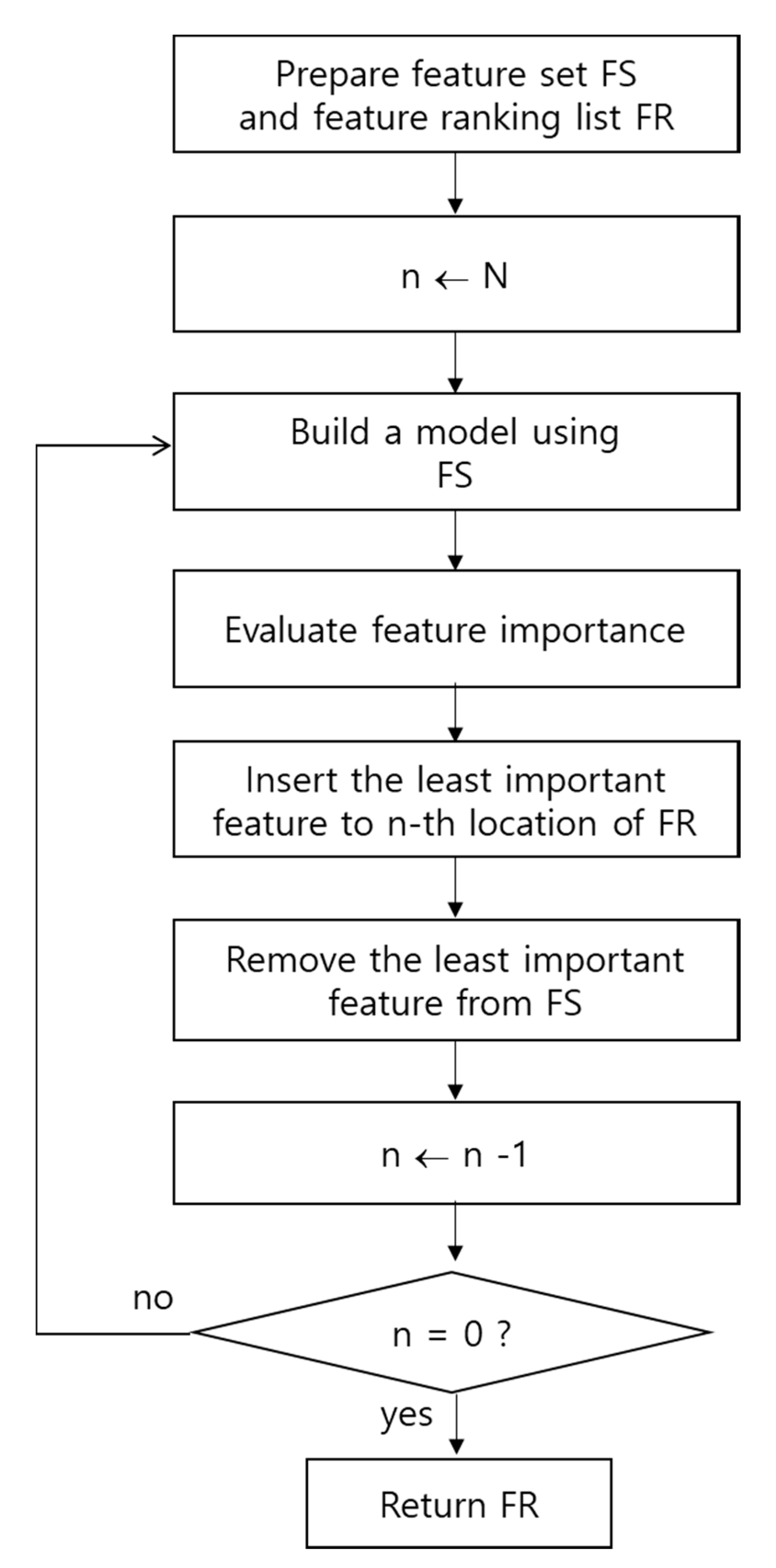
2.1. Idea of Hybrid Recursive Feature Elimination

In machine learning tasks, ensembles of different methods may produce higher performance than each individual method. Therefore, we can expect that an ensemble of RFEs will produce a better performance than a single RFE. Hybrid-RFE is an ensemble algorithm for feature selection that combines the SVM-RFE, RF-RFE, and GBM-RFE methods. Hybrid-RFE has two types of weighting functions. The first type is the simple sum of the feature weights from the three RFE methods. The second type reflects both feature weights and model accuracies from the three RFE methods.

Each feature weight obtained from the three RFE methods should be normalized before combining because their scales of weight values are different. The weighting functions of Hybrid-RFE are summarized in Figure 2.

2.2. Hybrid Method: Simple Sum

The simple sum function—W_Hss—is calculated by the sum of the normalized weights—${\overline{\mathit{W}}}_{\mathit{S}}$, ${\overline{\mathit{W}}}_{\mathit{R}}$, and ${\overline{\mathit{W}}}_{\mathit{G}}$—from SVM-RFE, RF-RFE, and GBM-RFE, respectively. Equation (6) describes the W_Hss function. In the equation, X is a feature set to be evaluated. The weight values w in a weight vector W are normalized by Equation (7):

$${\mathit{W}}_{\mathit{H}\mathit{s}\mathit{s}}\left(\mathit{X}\right)={\overline{\mathit{W}}}_{\mathit{s}}\left(\mathit{X}\right)+{\overline{\mathit{W}}}_{\mathit{R}}\left(\mathit{X}\right)+{\overline{\mathit{W}}}_{\mathit{G}}\left(\mathit{X}\right)$$

(6)

Normalizedw = (w − min(W))/(max(W) − min(W))

(7)

2.3. Hybrid Method: Weighted Sum

The weighted sum function considers both the weight values and model accuracy. Model accuracy refers to the classification accuracy obtained from the model. For this process, the given dataset is divided into a training set and test set. The training set is used to build a model and obtain the weight values for the features. The test set is used to obtain the classification accuracy of the model. Equation (8) describes the weighted sum function W_Hws. In this equation, SVM.acc, RF.acc, and GBM.acc represent the model accuracy of SVM-RFE, RF-RFE, and GBM-RFE, respectively.

$$\begin{array}{l}{\mathit{W}}_{\mathit{H}\mathit{s}\mathit{s}}\left(\mathit{X}\right)={\overline{\mathit{W}}}_{\mathit{s}}\left(\mathit{X}\right)\times SVM.acc+\\ {\overline{\mathit{W}}}_{\mathit{R}}\left(\mathit{X}\right)\times RF.acc+\\ {\overline{\mathit{W}}}_{\mathit{G}}\left(\mathit{X}\right)\times GBM.acc\end{array}$$

(8)

3. Results

3.1. Datasets

To compare the proposed method with the previous RFE methods, we chose eight benchmark datasets from the UCI Machine Learning Repository (http://archive.ics.uci.edu/ml/index.php) and the NCBI Gene Expression Omnibus repository (https://www.ncbi.nlm.nih.gov/geo/). The benchmark datasets are summarized in

Table 1. List of benchmark datasets.

No.	Dataset	# of Observations	# of Features	# of Classes
1	satellite	6435	36	6
2	messidor	351	33	2
3	sonar	208	60	2
4	messidor	1151	20	2
5	GDS1027	154	1000	4
6	GDS2546	167	1000	4
7	GDS2547	164	1000	4
8	GDS3715	109	1000	3

. The first four datasets are from UCI, and the rest are from NCBI. The UCI datasets contain a relatively small number of features. The NCBI datasets have numerous features and small numbers of observations (samples). Each feature contains the gene expression values of a specific gene. These are typical datasets that require feature selection as they contain more than 20,000 features. To save computing time, we randomly selected 1000 features from them.

3.2. Experiments

We compared the previous RFE methods (SVM-RFE, RF-RFE, GBM-RFE) and the proposed Hybrid-RFE method. Hybrid-RFE was tested using simple sum and weighted sum functions. All experiments were performed using R language (http://www.r-project.org). The SVM-RFE code was referenced from multiple SVM-RFE [11], and we implemented the code for the others as modified versions of SVM-RFE (See Supplementary Materials).

The performance evaluation metric for each method was the classification accuracy obtained on the selected features from the RFE methods. Four classification algorithms were used: k-nearest neighbor (KNN), SVM, RF, and naïve Bayes (NB). The default tuning parameters were used for each classifier.

Table 2. Classifiers and their corresponding R packages.

Classifier	R package
KNN	class
SVM	e1071
RF	randomForest
NB	e1071

lists these classifiers and their corresponding R packages.

Five-fold cross-validation was used not only to evaluate the accuracy of each classifier after feature selection, but also to perform the RFE process. In other words, the final feature importance list of an RFE method was calculated by averaging the five feature importance lists from each cross-validation fold.

All of our RFE algorithms have a “halve.aboves” parameter. If the number of features is larger than the parameter value, RFE removes half of the least important features from the feature list. This approach was suggested by [11] as a means to speed up the feature selection process. In the regular RFE process, only the least important feature was removed from the feature list. We set the “halve.aboves” parameter to 200.

3.3. Experimental Results

Using the feature importance ranking list from the three previous RFE methods and two proposed RFE methods, four classifiers were tested to find the best feature set that produced the highest classification accuracy. The results of the basic experiment are summarized in

Table 3. Experimental results.

Dataset	Algorithm	Accuracy	RFE Methods
		on Entire Feature Set	SVM-RFE	RF-RFE	GBM-RFE	Hybrid-RFE (SS) 1	Hybrid-RFE (WS) 2
satellite	KNN	0.904	0.904 (36)	0.904 (36)	0.904 (36)	0.907 (31)	0.904 (31)
	SVM	0.898	0.899 (27)	0.898 (36)	0.898 (36)	0.898 (35)	0.899 (31)
	RF	0.918	0.919 (36)	0.919 (36)	0.919 (36)	0.919 (36)	0.919 (33)
	NB	0.773	0.778 (24)	0.773 (36)	0.783 (11)	0.785 (18)	0.780 (10)
ionosphere	KNN	0.855	0.904 (19)	0.915 (12)	0.901 (21)	0.906 (10)	0.918 (12)
	SVM	0.949	0.951 (21)	0.939 (33)	0.949 (33)	0.952 (28)	0.958 (23)
	RF	0.923	0.938 (33)	0.938 (27)	0.929 (32)	0.932 (26)	0.933 (27)
	NB	0.724	0.781 (12)	0.858 (12)	0.808 (10)	0.849 (13)	0.835 (11)
sonar	KNN	0.815	0.856 (32)	0.831 (28)	0.859 (30)	0.854 (28)	0.840 (39)
	SVM	0.824	0.815 (55)	0.821 (31)	0.836 (48)	0.843 (52)	0.825 (44)
	RF	0.811	0.833 (54)	0.820 (29)	0.833 (57)	0.846 (27)	0.850 (44)
	NB	0.753	0.746 (42)	0.769 (33)	0.753 (60)	0.770 (42)	0.763 (35)
messidor	KNN	0.615	0.647 (10)	0.644 (10)	0.637 (16)	0.652 (11)	0.633 (10)
	SVM	0.710	0.710 (19)	0.710 (19)	0.710 (19)	0.710 (19)	0.710 (19)
	RF	0.690	0.702 (11)	0.697 (11)	0.689 (19)	0.709 (11)	0.699 (15)
	NB	0.610	0.610 (18)	0.610 (19)	0.613 (16)	0.610 (19)	0.610 (19)
GDS1027	KNN	0.812	0.802 (962)	0.807 (789)	0.803 (732)	0.833 (680)	0.825 (637)
	SVM	0.565	0.552 (68)	0.547 (361)	0.540 (52)	0.532 (360)	0.545 (103)
	RF	0.623	0.633 (943)	0.625 (971)	0.628 (791)	0.631 (978)	0.656 (477)
	NB	0.475	0.511 (218)	0.528 (804)	0.530 (896)	0.537 (798)	0.572 (132)
GDS2546	KNN	0.629	0.667 (684)	0.697 (12)	0.661 (95)	0.685 (161)	0.668 (11)
	SVM	0.706	0.730 (155)	0.712 (63)	0.731 (266)	0.727 (140)	0.732 (44)
	RF	0.719	0.712 (847)	0.761 (25)	0.725 (13)	0.718 (11)	0.742 (125)
	NB	0.711	0.743 (61)	0.729 (637)	0.740 (540)	0.746 (246)	0.748 (46)
GDS2547	KNN	0.64	0.644 (680)	0.632 (932)	0.660 (907)	0.656 (257)	0.689 (231)
	SVM	0.607	0.648 (708)	0.653 (421)	0.637 (870)	0.653 (55)	0.644 (84)
	RF	0.672	0.679 (852)	0.678 (951)	0.704 (377)	0.685 (884)	0.689 (498)
	NB	0.69	0.704 (806)	0.680 (848)	0.705 (265)	0.698 (395)	0.699 (814)
GDS3715	KNN	0.799	0.821 (244)	0.804 (50)	0.813 (191)	0.837 (347)	0.804 (92)
	SVM	0.816	0.848 (133)	0.846 (125)	0.854 (691)	0.863 (110)	0.863 (317)
	RF	0.816	0.848 (917)	0.849 (761)	0.840 (742)	0.847 (505)	0.861 (306)
	NB	0.652	0.773 (841)	0.773 (971)	0.775 (716)	0.775 (488)	0.790 (87)

¹ simple sum function, ² weighted sum function

. Each cell expresses the highest classification accuracy, and the number of selected features is shown in parentheses next to the accuracy value. For example, 0.904 (36) from SVM-RFE and KNN indicates that the SVM classifier produced the highest accuracy of 0.904 when it used the first 36 features from the SVM-RFE feature ranking list. The data in bold in the table represent the top values for a specific classifier. If two or more methods produced equal top accuracy, the method that used the least number of selected features was chosen.

From Table 3, it is evident that the top values were mainly produced by the two proposed methods. This means that the feature ranking lists generated by the proposed methods were better than those generated using the previous methods. The frequency of top accuracies for the compared RFE methods are summarized in

Table 4. Frequency of top accuracy for RFE methods.

SVM-RFE	RF-RFE	GBM-RFE	Hybrid-RFE (ss)	Hybrid-RFE (ws)
2	4	4	10	11

. The frequencies of Hybrid-RFE with the simple sum function and weighted sum were 10 and 11, respectively (total of 21). The frequencies of SVM-RFE, RF-RFE, and GBM-RFE were 2, 4, and 4, respectively. In our experiment, Hybrid-RFE with the weighted sum function showed the best performance, whereas SVM-RFE showed the worst performance.

If two RFE methods A and B produce the same classification accuracies and the numbers of selected features are 15 and 10, respectively, method B is more efficient than method A. The ideal feature selection method produces a small feature subset size and high classification accuracy. Therefore, we compared the average size of the set of selected features from the five RFE methods. The results are summarized in

Table 5. Average number of selected features from the GDS datasets.

SVM-RFE	RF-RFE	GBM-RFE	Hybrid-RFE (ss)	Hybrid-RFE (ws)
570	545	509	401	250

. Only the GDS datasets were used in the comparison because the others have a small number of features in the original datasets. The proposed Hybrid-RFE methods were more efficient than previous RFE methods. In particular, Hybrid-RFE with a weighted sum function produced a remarkably small feature subset.

4. Discussion

There is no “super” feature selection method for every dataset. Each dataset has unique characteristics that influence the working mechanisms of the feature selection method. Therefore, several feature selection methods need to be tested. Furthermore, there is no relationship between classifiers and feature selection methods—it is not known which feature selection method is best for SVM or which classifier is best for GBM-RFE. Therefore, it is necessary to check combinations of classifiers and feature selection methods in order to build a high-performance classification model. A small number of good classifiers and feature selection methods are required in order to reduce the experimentation time.

The proposed Hybrid-RFE method has been shown to provide better performance than previous RFE methods. It can thus be considered first if feature selection is required. The key point of Hybrid-RFE is the weighting function that combines different RFE weights. If we can find a more efficient weighting function, Hybrid-RFE can be improved. Hybrid-RFE combines the normalized weights of different RFEs and adopts “local” normalization. If we could develop “global” normalization, feature weights from several RFEs could be more effectively combined. Furthermore, feature interaction and feature dependency are important factors for feature selection. We have not yet found a way to measure these factors and combine them with feature importance. These are potential topics for further research.

References

1. Tang, J.; Alelyani, S.; Liu, H. Feature Selection for Classification: A Review; Chapman and Hall/CRC: New York, NY, USA, 2014; pp. 37–64. [Google Scholar] [CrossRef]
2. Bellman, R. Dynamic Programming, 6th ed.; Princeton Univ. Press: Prinston, NJ, USA, 1957; p. 4. [Google Scholar]
3. Kumar, V.; Minz, S. Feature selection: A literature review. SmartCR 2014, 4, 211–229. [Google Scholar] [CrossRef]
4. Tang, J.; Alelyani, S.; Liu, H. Feature selection for classification: A review. Data Class Algor. Appl. 2014, 37, 1–29. [Google Scholar]
5. Bolón-Canedo, V.; Sánchez-Marono, N.; Alonso-Betanzos, A.; Benítez, J.M.; Herrera, F. A review of microarray datasets and applied feature selection methods. Inform. Sci. 2014, 282, 111–135. [Google Scholar] [CrossRef]
6. Ang, J.C.; Mirzal, A.; Haron, H.; Hamed, H.N.A. Supervised, unsupervised, and semi-supervised feature selection: A review on gene selection. IEEE/ACM Trans. Comput. Biol. Bioinform. 2015, 13, 971–989. [Google Scholar] [CrossRef] [PubMed]
7. Saeys, Y.; Inza, I.; Larrañaga, P. A review of feature selection techniques in bioinformatics. Bioinformatics 2007, 23, 2507–2517. [Google Scholar] [CrossRef] [PubMed] [Green Version]
8. Liu, H.; Motoda, H. Computational Methods of Feature Selection; Chapman and Hall/CRC: New York, NY, USA, 2007. [Google Scholar]
9. Liu, H.; Yu, L. Toward integrating feature selection algorithms for classification and clustering. IEEE Trans. Knowl. Data Eng. 2005, 17, 491. [Google Scholar]
10. Guyon, I.; Weston, J.; Barnhill, S.; Vapnik, V. Gene selection for cancer classification using support vector machines. Mach. Learn. 2002, 46, 389–422. [Google Scholar] [CrossRef]
11. Duan, K.B.; Rajapakse, J.C.; Wang, H.; Azuaje, F. Multiple SVM-RFE for gene selection in cancer classification with expression data. IEEE Trans. Nanobiosci. 2005, 4, 228–234. [Google Scholar] [CrossRef] [PubMed]
12. Mundra, P.A.; Rajapakse, J.C. SVM-RFE with MRMR filter for gene selection. IEEE Trans. Nanobiosci. 2009, 9, 31–37. [Google Scholar] [CrossRef] [PubMed]
13. Zhou, X.; Tuck, D.P. MSVM-RFE: Extensions of SVM-RFE for multiclass gene selection on DNA microarray data. Bioinformatics 2007, 23, 1106–1114. [Google Scholar] [CrossRef] [PubMed] [Green Version]
14. Tang, Y.; Zhang, Y.Q.; Huang, Z. Development of two-stage SVM-RFE gene selection strategy for microarray expression data analysis. IEEE/ACM Trans. Comput. Biol. Bioinform. 2007, 4, 365–381. [Google Scholar] [CrossRef] [PubMed]
15. Ding, Y.; Wilkins, D. Improving the performance of SVM-RFE to select genes in microarray data. BMC Bioinform. 2006, 7, S12. [Google Scholar] [CrossRef] [PubMed] [Green Version]
16. Granitto, P.M.; Furlanello, C.L.; Biasioli, F.; Gasperi, F. Recursive feature elimination with random forest for PTR-MS analysis of agroindustrial products. Chemom. Intell. Lab. Syst. 2006, 83, 83–90. [Google Scholar] [CrossRef]
17. Hierpe, A. Computing Random Forests Variable Importance Measures (VIM) on Mixed Continuous and Categorical Data. Master’s Thesis, KTH Royal Institute of Technology, Stockholm, Sweden, 2016. [Google Scholar]
Figure 1. Process of feature-importance-based recursive feature elimination (RFE). N denotes the number of features.
Applsci 10 03211 g001
Figure 2. Two types of weighting functions of Hybrid-RFE.
Applsci 10 03211 g002