Abstract
Superpixel segmentation has become a crucial tool in many image processing and computer vision applications. In this paper, a novel content-sensitive superpixel generation algorithm with boundary adjustment is proposed. First, the image local entropy was used to measure the amount of information in the image, and the amount of information was evenly distributed to each seed. It placed more seeds to achieve the lower under-segmentation in content-dense regions, and placed the fewer seeds to increase computational efficiency in content-sparse regions. Second, the Prim algorithm was adopted to generate uniform superpixels efficiently. Third, a boundary adjustment strategy with the adaptive distance further optimized the superpixels to improve the performance of the superpixel. Experimental results on the Berkeley Segmentation Database show that our method outperforms competing methods under evaluation metrics.
1. Introduction
Dividing an image into several simple connected regions with perceptual meanings is called superpixels. Superpixels can represent images more concisely and efficiently than pixels, which can significantly reduce the complexity of subsequent image processing. After the concept of superpixels was proposed by Ren and Malik [1] in 2003, the simplified image expression became a key step in many computer vision tasks, such as segmentation [2,3,4,5,6], saliency detection [7,8,9], object recognition [10,11], modelling [12,13], 3D reconstruction [14], and other vision tasks [15,16,17]. For these applications, the high-quality superpixels are desired to meet the following properties:
- Each superpixel is a simple single connected area with the regular shape.
- Superpixels should adhere well to the image boundaries and pixels inside the superpixels should have homologous characteristics.
- The density of superpixels should be adaptive to local image content.
- The superpixels algorithms should be fast to compute and memory efficient.
The superpixel segmentation algorithms can be roughly divided into two categories: Graph-based methods and clustering-based methods. Graph-based methods treat each pixel as a vertex in the graph. The similarity between adjacent pixels is considered as the weight of the edge. The normalized cut (N-cut) algorithm [18] recursively partitions the pixel graph using contour and texture information in the image. Felzenszwalb and Huttenlocher [19] proposed a superpixel generation method based on the minimum spanning tree (FH). Moore et al. [20] generated superpixels (SL) by searching the minimum path from the horizontal and vertical directions. Veksler et al. [21] generated superpixels (Graph Cut) by half-overlapping square patches of the same size covered on the image. Liu et al. [22] presented a graph-based approach (ERS), which combines the entropy rate of a random walk with and a balancing function for superpixel segmentation. SEEDS [23] generates superpixels by iteratively modifying the initial approximate boundaries of superpixels according to the energy function.
The clustering-based methods define a distance measure to evaluate the similarity between pixels and generate superpixels by iteratively assigning pixels to the most similar seeds until some convergence criteria are reached. TurboPixels [24] is a geometric flow method (TP), which regularly places the seeds on images and grows the superpixels by level-set. This method can make the size of superpixels uniform, but it consumes more time than other superpixel methods.
Zeng et al. [25] proposed structure-sensitive superpixels (SSS) according to the geodesic distance computed from geometric flows. SSS can effectively describe the nonhomogenous features in images by the superpixel size. However, the computational cost of SSS is even higher than that of TP.
Achanta et al. [26] proposed an algorithm, simple linear iterative clustering (SLIC), to generate superpixels. SLIC uniformly places the initial cluster centers on the geometric center of the regular grids. By limiting the search range of the k-means algorithm, the computational complexity of the SLIC is greatly reduced. To further improve the performance of SLIC, Achanta and Susstrunk [27] proposed simple non-iterative clustering (SNIC) to compute superpixels with one iteration.
Liu et al. [28] proposed manifold SLIC (MSLIC), which expands SLIC to generate content-sensitive superpixels. MSLIC maps a five-dimensional image space to a two-dimensional manifold for computing restricted centroidal Voronoi tessellation under the Euclidean metric. As an improvement of MSLIC, the authors proposed intrinsic manifold SLIC [29] (IMSLIC) to compute a centroidal Voronoi tessellation under the geodesic distance instead of Euclidean distance on the image manifold.
Shen et al. [30] presented the lazy random walk (LRW) method to evaluate the probabilities between a seed and its neighbor pixels. The authors [31] also proposed a real-time superpixel segmentation method (DBSCAN) to apply density-based spatial clustering. Small initial superpixels are further merged with adjacent superpixels to ensure connected superpixels.
Li and Chen [32] proposed the linear spectral clustering (LSC) to generate superpixels based on simple k-means clustering. The algorithm maps a five-dimensional color space into a ten-dimensional space, resulting in superpixels with high boundary adherence.
All the above clustering-based methods usually consist of two steps: (1) Regular initialization of seeds to generate superpixel, and (2) update seeds to the center of mass. The results of this algorithm depend on the initial position of seeds, and the seed regular initialization ignores the content sensitivity. To address this issue, we propose a novel superpixel segmentation algorithm, which adopts the image local entropy and the boundary adjustment strategy to generate superpixels. In summary, the contribution of this paper includes the following three respects:
- The seeds initialized by most cluster-based superpixel algorithms are spatially uniform. Our method introduces image entropy at seeds sampling, which aims at generating content-sensitive superpixels to improve the accuracy of superpixel segmentation. The image local entropy can well measure the content sensitivity of the image and can initialize the seeds at a lower computational cost.
- We used boundary adjustment to optimize superpixels. Adaptive boundary adjustment can generate regular superpixels in sparse content areas and superpixels with good boundary adherence in dense content areas, and the boundary adjustment can quickly converge.
- The proposed algorithm was evaluated on the Berkeley Segmentation Database (BSDS 500) [33]. Compared with other five methods, the algorithm achieved better segmentation accuracy while ensuring superpixel compactness.
The rest of the paper is organized as follows. The Section 2 introduces our method and analyzes the parameters in detail. The experimental results, compared with the five representative methods, are shown in Section 3. Experimental results are discussed in Section 4. In Section 5, we show the foreground segmentation performance of the superpixel algorithm proposed in contour closure. Finally, a brief summary is made in Section 6.
2. Materials and Methods
This paper develops a novel method for generating content-sensitive superpixels, which improves the performance of segmentation algorithms. The proposed algorithm has three phases. The first phase is seed sampling for adaptive image content. The second phase is clustering superpixels based on the minimum spanning tree algorithm. The third phase is the boundary adjustment phase, in which the distance measure of adaptive weights is adopted to improve the segmentation quality.
2.1. Seed Sampling Strategy
Any natural image contains a lot of uneven image information. The change in the local color intensity of the image reflects the change in the amount of local information. Therefore, it is but natural to place more seeds in content-dense regions of the image and to place fewer seeds in content-sparse regions of the image. However, the uniformity of seeds is also strongly important for the compactness of superpixels. Then, the proposed seeds distribution strategy based on image local entropy achieved a balance between the content sensitivity and uniformity of seeds. The heterogeneity of each pixel was captured using Normalized Shannon Entropy. The entropy operator calculates the entropy of the pixel value in the neighbor center. Let the pixel gray values in the center and the N neighbor pixels be a0, a1, a2, …, aN, respectively. The entropy operator is given in Table 1.

Table 1.
Entropy operator.
The entropy H was normalized so that . For color images in the CIELAB color space , the image local entropy is defined as
where
Both brightness information and tone information were used to measure the local entropy carried by natural color images. Therefore, when the brightness or the color tone of the region changed greatly, the entropy value of the color image was small. The part of the image should contain more information when the color intensity of the part of the image changes drastically, and vice versa. For neighborhood center i, the local information of each pixel I(i) is defined as
where ω and γ are scaling parameters.
We outline seed sampling strategy in Algorithm 1. Different from the placement method of simple regular grids seeds [26] and two-level quad-tree split-up seeds [25], the proposed approach considered the local information of the image in the process of placing seeds. In order to make each superpixel contain an approximate amount of image information, the information interval was , where n is the number of pixels in the image and k is the desired number of superpixels. The images were scanned from left to right and from top to bottom, and the pixels were added that were four- or eight-connected to the currently growing region. When the scanned pixels reached the information interval, the seed was placed. For an initial superpixel Si, its position center is
| Algorithm 1. Seed sampling strategy |
| Input: An image 𝐼 of n pixels, the desired number of superpixels k, and the parameters γ and ω |
| Output:k seeds of the image I |
| Calculate the local information of each pixel |
| Calculate information interval of image I |
| for each pixel pi do |
| if the pixel is not scanned then |
| Store pi as region Si |
| for each connected neighbor pj of Si do |
| if the pixel is not scanned then |
| Add pj to region Si |
| if then |
| break |
| end if |
| end if |
| end for |
| end if |
| Place seed using Equation (4) |
| end for |
2.2. Minimum Spanning Tree Clustering
An image can be converted to an undirected graph , whose pixels in the image are the vertices and the value of each edge evaluates the similarity between the two vertices . Let k be the number of superpixels to be divided, the superpixel segmentation task is broken up the undirected graph into k disjoint subgraphs , where and .
The proposed algorithm is a kind of bottom-up pixel aggregation method, which grows regions based on the Prim method [34]. The Prim algorithm is a greedy algorithm that finds the minimum spanning tree for a weighted undirected graph. Suppose a graph has n vertices, and the goal is to aggregate the vertices into a forest with k trees. Starting from the initial seeds, the algorithm adds the least cost connection from the tree to the vertex in each step. Similar to SLIC [26], a distance measure was adopted in five-dimensional space. In the spatial space and CIELAB color space , the distance of two vertices v1 and v2 is defined as
where is a normalization parameter. For an image of n pixels, the value of is set to be . The value of λ is set by the user. λ weighs the relative importance of the color distance term and spatial distance term. The larger the λ value is, the more regular the generated superpixels are. The smaller the λ value is, the boundary adherence better the generated superpixels are.
The Prim algorithm only considers the distance between two vertices on the tree border during the aggregation process. This metric is extremely sensitive to noise. The average attributes of the tree are used to calculate the distance, which not only simplifies the calculation of the shortest path distance in the neighbor, but also improves the robustness of the Prim algorithm. After running the Prim algorithm, k trees representing k superpixels are generated. For a superpixel Si, its average attribute is given by
The average attribute replaces the seed to calculate the distance. Figure 1 illustrates this aggregation process of superpixels. The process of minimum spanning tree clustering is summarized in Algorithm 2.
| Algorithm 2. Minimum Spanning Tree Clustering |
| Input: An image 𝐼 of n pixels, k initial locations generated in Algorithm 1 and the weight parameter λ |
| Output: Initial Superpixel label map L |
| Initialize |
| Initialize by extracting the features of the initial locations |
| for each centroid do |
| Vertex |
| Push v on priority queue Q |
| end for |
| whiledo |
| remove vi from the priority queue Q |
| Update the centroid using Equation (6) |
| for Each connected neighbor vj of vi do |
| Calculated distance of vj and vi using Equation (5) |
| Create the Vertex |
| if then |
| Push vj on Q |
| end if |
| end for |
| end while |
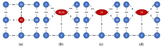
Figure 1.
Illustration of the aggregation process of superpixels. The vertices represent pixels and the edges represent similarities. (a)The vertex 15 is the nearest neighbor of the tree (red vertex 11), (b) the tree aggregates the nearest neighbor, (c) update the average attribute of the tree, (d) expand the search scope of the tree and find the next nearest neighbor(vertex 9).
2.3. Boundary Adjustment
The preliminary segmentation results were formed at one time and further optimization was required. In Figure 2, the shape of the superpixel was not regular enough, especially in the content-sparse region. There were several under-segmentation errors in the area pointed by the red arrow in the image. It can be seen that boundary adjustment significantly improved the compactness and boundary adherence of superpixels.
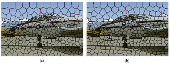
Figure 2.
Image segmentation results with 400 superpixels. (a) Superpixel segmentation results after minimum spanning tree clustering, (b) superpixel segmentation results after boundary adjustment.
The boundary pixels of the initial superpixels were allocated to obtain better compactness and boundary adherence. Among pixels connected to Si, the pixels that do not belong to Si are boundary pixels. For each boundary pixel, calculate the distance between the boundary pixel and the adjacent superpixel, and assign the boundary pixel to the superpixel which is nearest to it. Boundary adjustment is an iterative process. The iteration is terminated when the set number of iterations is reached.
In the distance Equation (5), the color distance term affects the adherence of superpixels boundary, and spatial distance term affects the compactness of superpixels. To enhance the content sensitivity of superpixels, we define the new distance measurement as follows:
When the value I(i) is higher, the color distance is more considered. When the value I(i) is lower, the spatial distances should be more considered.
Boundary adjustment does not guarantee the superpixel connectivity. In the procedure, a superpixel may be split into several unconnected sub-superpixels. Connectivity is taken into account of the procedure of boundary adjustment and additional steps are not required. For too small sub-superpixels, they will merge with the nearest superpixel. The pseudo code of boundary adjustment is presented Algorithm 3.
| Algorithm 3. Boundary adjustment |
| Input: Initial Superpixel label map L and the maximum number of iterations Maxiter |
| Output: Optimized Superpixel label map L |
| While iter < Maxiter do |
| for each superpixel Si do |
| for each boundary vertex vi do |
| for Each connected neighbor vj of vi that are not in Si do |
| Get the superpixel Sj which vj belongs to |
| Compute and using Equation (7) |
| if < then |
| Update Ci and Cj using Equation (6) |
| Update the boundary vertices |
| end if |
| end for |
| end for |
| end for |
| end while |
For an image with n pixels, it is obvious that the complexity of the image local entropy and the seed sampling strategy are О(n). In the minimum spanning tree clustering phase, the number of pixels in the priority queue is much smaller than n. Thereby, the impact of priority queues on computational complexity is not very obvious. In the boundary adjustment stage, the computational cost in each iteration is О(), in which is the number of boundary pixels. In practice, . In the comprehensive analysis, the proposed algorithm is of linear complexity О(n).
2.4. Datasets and Performance Metrics
We adopted the commonly used evaluation metrics in the literature of superpixel segmentation to evaluate superpixel segmentation algorithms, including boundary recall (BR), achievable segmentation accuracy (ASA), and under-segmentation error (USE). The BSDS 500 [33] consisted of 500 images with manually labeled ground truth segmentations. In the following experiments, the methods were evaluated using the average performance metrics of five hundred images in the BSDS 500 [33].
Boundary recall (BR) measures the fraction of the ground truth boundary identifications. A high BR represents the better boundary adherence with respect to the ground truth boundaries. Given a ground truth boundary sets B(g) and the superpixel boundary sets B(s), then BR is defined as:
Let FN (B(g), B(s)) and TP (B(g), B(s)) be the number of false negative and true positive boundary pixels. B(s) is matched to B(g) within a local neighbor with size (2r + 1) × (2r + 1). In practice, r is set to 1.
Achievable segmentation accuracy (ASA) computes the upper bound of accuracy using superpixels as preprocessing step. Denote a ground truth segmentation of an image as and a superpixel segmentation as . The ASA metric is defined as follows:
where is the number of a superpixel in pixel. In general, a high ASA demonstrates that superpixels match the objects well in the image.
Under-segmentation error (USE) measures the “leakage” of superpixels from the ground truth boundaries, which is calculated by:
where n is the total number of pixels in the image. Each superpixel was assigned to the ground truth segments with the largest overlap, and only the “leakage” with respect to other ground truth segments was considered. Therefore, USE implicitly also measures boundary adherence. A lower USE refers to that superpixels overlap with a ground truth segmentation more accurately.
2.5. Parameter Selection
In the proposed method, γ, ω, λ, and Maxiter should be set in advance. The following experiments use various values to investigate the parameters.
The measure of image information contains two parameters, γ and ω. γ is used to adjust the uniformity and content sensitivity of the seeds. As shown in Figure 3, with the increasing values of γ, the value of performance metrics changes significantly because small γ values imply the seeds are too sensitive to the image content and concentrated in complex areas while ignoring other areas. When γ becomes too large, the distribution of seeds tends to regular grid seeds, and the content sensitivity is ignored. ω is used to adjust the proportion of the color term in Equation (7). In practice, we truly use their product, . Approximately, the values of I(i) fall in the interval [0, p]. As shown in Figure 4, when p increases, more detailed information is considered and the resulting superpixels are more irregular.
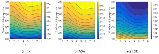
Figure 3.
The performance metrics of our approach with different γ values.
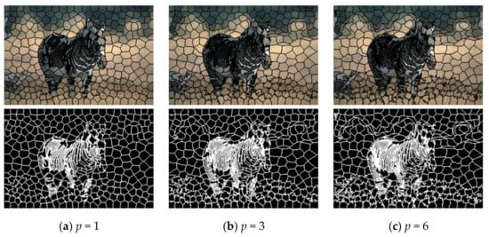
Figure 4.
Superpixel segmentation results with different p values.
λ represents the weight parameters of the distance measure in the stage of minimum spanning tree clustering. Particularly, when λ→∞, the generated superpixels are regularly grid only related to the position of the initial seeds. When λ = 0, the pixels with similar colors are clustered to generate irregular superpixels. The trend is shown in Figure 5. Figure 6 shows the average values of BR, ASA, and USE on the BSDS 500 for different λ values when K = 400. Overall, the performance metrics becomes worse as the value of λ increases.
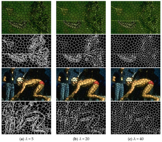
Figure 5.
Superpixel segmentation results with different λ values.
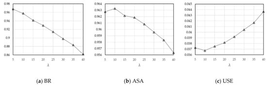
Figure 6.
The performance metrics of our approach with different λ values at k = 400.
The number of iterations Maxiter can balance time cost and performance. The metrics with Maxiter are shown in Figure 7. It is easy to find that our algorithm can quickly converge after two iterations. More iterations will only increase time consumption. Also shown in Figure 2, the superpixels became more compact after iterations.
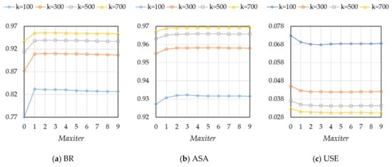
Figure 7.
The performance metrics of our approach for different Maxiter values.
From the discussion above, we select γ = 6 and Maxiter = 3, where achieve the best performance. Considering the accuracy and compactness of superpixels, we empirically select λ = 20 and p = 3.
3. Results
The proposed algorithm was implemented in C++ and tested on a PC with an Intel i5-8300H CPU (2.30 GHz) and 8GB RAM. The performance of the proposed algorithm was compared with the five representative superpixel generation algorithms, including SLIC [26], SNIC [27], ERS [22], LSC [32], and FH [19]. We used the implementations available online for all other methods. To ensure segmentation performance, all algorithms were run on the recommended parameters. The comparison experiment results on BSDS 500 [33] are shown in Figure 8. As a preprocessing step for image processing, the time cost was also an important indicator. In Figure 8d, we also compared the efficiency in the average running time per image. Table 2 presents the mean and standard deviation performance metrics at k = 400. A visual comparison is displayed in Figure 9.
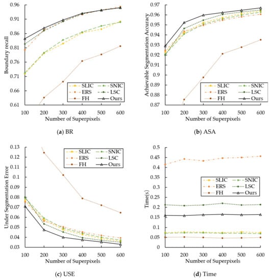
Figure 8.
Quantitative evaluation of different superpixel segmentation algorithms.
Table 2.
Performance metrics of different superpixel segmentation algorithms at k = 400.
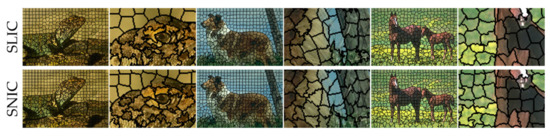
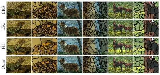
Figure 9.
Visual comparison of superpixel segmentation results using different algorithms.
A good initialization is essential for superpixel algorithms. In Section 2.1, we propose a seed sampling strategy different from regular grid initialization, which introduces image entropy into seed sampling strategy to optimize the content sensitivity of the seed. Furthermore, the content initialization compares with regular initialization in the proposed method on the entire BSDS 500 dataset. The results under the three metrics (i.e., USE, BR, and ASA) are reported in Figure 10, which shows that our sampling strategy is better than regular grid initialization.
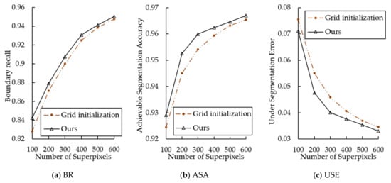
Figure 10.
The metrics value comparison of our seed sampling strategy and grid initializations.
4. Discussion
Referring to the plots in Figure 8, our method is superior to the other five methods in terms of ASA and USE. The LSC, ERS, and our method exhibit high performance on BR. However, our approach is more competitive at a lower set number of superpixels. As a preprocessing step, generating a lower number of high-quality superpixels is more helpful for subsequent tasks. From Figure 8 and Table 2, it can be seen that the proposed method is comparable to the other five representative methods in terms of boundary adherence.
Figure 9 shows the visual results of superpixel segmentation using these algorithms. Enlarge the local segmentation results for detailed inspection. Visually, our method had the most satisfactory segmentation results for different types of images. SLIC, SNIC, and our method showed the best compactness. However, compared with the proposed algorithm, SLIC and SNIC had weaker boundary adherence. The boundary adherence of ERS was very competitive, but the compactness of ERS was not satisfactory. LSC produced competitive results and performed well in compactness and boundary adherence. LSC introduces global information to generate superpixels, which makes it requires 20 iterations. From Figure 8d, LSC took longer to run than our method. In addition, our method can exceed the performance of LSC by adjusting parameters, but it sacrifices compactness. Superpixels generated by FH and the proposed method exhibited content sensitivity. Due to the lack of compactness constraints, the superpixels produced by FH were extremely irregular and under-segmented in content-rich areas. The results show that the algorithm achieves good boundary adherence while ensuring good compactness.
5. Application to Image Contour Closure
We investigated the effect of segmentation using different superpixels in image contour closure applications. Superpixel is a preprocessing step to reduce the complexity of subsequent image tasks. Levinshtein et al. [6] proposed an energy framework to search for a subset of superpixels to obtain the contour of strong edge support in an image. The energy framework proposed by Levinshtein et al. was used to compare six superpixel algorithms. The energy framework was applied to the Weizmann Segmentation Evaluation Database (WSED) [35], which consists of 100 images with human-annotated ground truth segmentations for each image. The average F-measure, precision, and recall are summarized in Table 3. Figure 11 also shows the qualitative results of the four examples. Both quantitative and qualitative results show that the proposed method has good foreground segmentation performance.
Table 3.
Performance metrics of the framework on WSED.
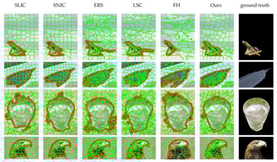
Figure 11.
Visual comparison of contour closure results on four examples in Weizmann Segmentation Evaluation Database (WSED). The superpixel boundaries are shown in green, and the closure contours are shown in red.
6. Conclusions
In this paper, we present a content-sensitive superpixel generation method with boundary adjustment, which generates compact superpixels that are adapted to image content. Owing to the uneven distribution of seeds, compared to other seed-based methods, the proposed algorithm is more sensitive to the content of the image. The approach tends to generate relatively small and irregular superpixels in complex regions for better boundary adherence, and generates relatively large regular superpixels in flat regions to improve computational efficiency. Taking advantage of boundary adjustment, the proposed algorithm provides results can adapt well to structure changes in natural images. We compared the proposed algorithm with five representative methods on the BSDS 500 dataset. The experimental results demonstrate that superpixels generated by the proposed method outperform the five superpixel algorithms in terms of USE, BR, and ASA. In the future, we will further research the algorithm in a noisy environment. In addition, we plan to apply this approach to applications that require content-sensitive superpixel algorithms.
Author Contributions
Conceptualization, D.Z. and W.B.; Formal analysis, J.R.; Methodology, D.Z., W.B. and X.X.; Software, D.Z. and Z.Z.; Supervision, G.X. and X.X.; Writing—review & editing, G.X. and J.R. All authors have read and agreed to the published version of the manuscript.
Funding
This work was supported in part by Shanxi International Cooperation Project (No. 201803D421039), Key Research and Development Plan of Shanxi Province (No. 201703D111027, No. 201703D111023), the Natural Science Foundation of Shanxi Province (No. 201801D121144, No. 201801D221190), and the Hundreds Talent Program of Shanxi Province, China. This work was also partially supported by the Shaanxi Natural Science Basic Research Project under Grant 2017JQ6058 and the Scientific Research Program funded by Shaanxi Provincial Education Department, China, under Grant 19JK0364.
Conflicts of Interest
The authors declare no conflict of interest.
References
- Ren, X.; Malik, J. Learning a classification model for segmentation. In Proceedings of the Ninth IEEE International Conference on Computer Vision, Nice, France, 13–16 October 2003; Volume 1, pp. 10–17. [Google Scholar]
- Ning, J.; Zhang, L.; Zhang, D.; Wu, C. Interactive image segmentation by maximal similarity based region merging. Pattern Recognit. 2010, 43, 445–456. [Google Scholar] [CrossRef]
- Li, Z.; Wu, X.-M.; Chang, S.-F. Segmentation using superpixels: A bipartite graph partitioning approach. In Proceedings of the 2012 IEEE Conference on Computer Vision and Pattern Recognition IEEE, Providence, RI, USA, 16–21 June 2012; pp. 789–796. [Google Scholar]
- Shen, J.; Peng, J.; Dong, X.; Shao, L.; Porikli, F. Higher-Order Energies for Image Segmentation. IEEE Trans. Image Proc. 2017, 26, 4911–4922. [Google Scholar] [CrossRef] [PubMed]
- Dong, X.; Shen, J.; Shao, L.; Gool, L.V. SubMarkov Random Walk for Image Segmentation. IEEE Trans. Image Proc. 2016, 25, 516–527. [Google Scholar] [CrossRef] [PubMed]
- Levinshtein, A.; Sminchisescu, C.; Dickinson, S. Optimal Image and Video Closure by Superpixel Grouping. Int. J. Comput. Vis. 2012, 100, 99–119. [Google Scholar] [CrossRef]
- Perazzi, F.; Krahenbuhl, P.; Pritch, Y.; Hornung, A. Saliency Filters: Contrast Based Filtering for Salient Region Detection. In Proceedings of the 2012 IEEE Conference on Computer Vision and Pattern Recognition, Providence, RI, USA, 16–21 June 2012. [Google Scholar]
- Wang, W.; Shen, J.; Shao, L. Video Salient Object Detection via Fully Convolutional Networks. IEEE Trans. Image Proc. 2018, 27, 38–49. [Google Scholar] [CrossRef] [PubMed]
- Wang, W.; Shen, J.; Shao, L. Consistent Video Saliency Using Local Gradient Flow Optimization and Global Refinement. IEEE Trans. Image Proc. 2015, 24, 4185–4196. [Google Scholar]
- Cour, T.; Shi, J. Recognizing objects by piecing together the segmentation puzzle. In Proceedings of the 2007 IEEE Conference on Computer Vision and Pattern Recognition IEEE, Minneapolis, MN, USA, 17–22 June 2007; pp. 1–8. [Google Scholar]
- Mori, G.; Ren, X.; Efros, A.A.; Malik, J. Recovering Human Body Configurations: Combining Segmentation and Recognition. In Proceedings of the 2004 IEEE Conference on Computer Vision and Pattern Recognition, Washington, DC, USA, 27 June–2 July 2004; pp. 326–333. [Google Scholar]
- He, X.; Zemel, R.S.; Ray, D. Learning and Incorporating Top-Down Cues in Image Segmentation. In Proceedings of the 2006 European Conference on Computer Vision, Graz, Austria, 7–13 May 2006; Volume 3951, pp. 338–351. [Google Scholar]
- Nwogu, I.; Corso, J.J. (BP)2: Beyond pairwise Belief Propagation labeling by approximating Kikuchi free energies. In Proceedings of the 2008 IEEE Conference on Computer Vision and Pattern Recognition, Anchorage, AK, USA, 24–26 June 2008; pp. 1–8. [Google Scholar]
- Hoiem, D.; Efros, A.A.; Hebert, M. Automatic photo pop-up. ACM Trans. Gr. 2005, 24, 577–584. [Google Scholar]
- Alexe, B.; Deselaers, T.; Ferrari, V. Measuring the Objectness of Image Windows. IEEE Trans. Pattern Anal Mach. Intell. 2012, 34, 2189–2202. [Google Scholar] [CrossRef] [PubMed]
- Bodis-Szomoru, A.; Riemenschneider, H.; Gool, L.V. Superpixel meshes for fast edge-preserving surface reconstruction. In Proceedings of the 2015 IEEE Conference on Computer Vision and Pattern Recognition, Boston, MA, USA, 7–12 June 2015; pp. 2011–2020. [Google Scholar]
- Lim, J.; Han, B. Generalized background subtraction using superpixels with label integrated motion estimation. In Proceedings of the 2014 European Conference on Computer Vision, Zurich, Switzerland, 6–12 September 2014; pp. 173–187. [Google Scholar]
- Shi, J.; Malik, J. Normalized cuts and image segmentation. IEEE Trans. Pattern Anal. Mach. Intell. 2000, 22, 888–905. [Google Scholar]
- Felzenszwalb, P.F.; Huttenlocher, D.P. Efficient graph-based image segmentation. Int. J. Comput. Vis. 2004, 59, 167–181. [Google Scholar] [CrossRef]
- Moore, A.P.; Prince, S.J.; Warrell, J.; Mohammed, U.; Jones, G. Superpixel lattices. In Proceedings of the 2008 IEEE Conference on Computer Vision and Pattern Recognition IEEE, Anchorage, AK, USA, 23–28 June 2008; pp. 1–8. [Google Scholar]
- Veksler, O.; Boykov, Y.; Mehrani, P. Superpixels and Supervoxels in an Energy Optimization framework. In Proceedings of the European Conference on Computer Vision, Crete, Greece, 5–11 September 2010; pp. 211–224. [Google Scholar]
- Liu, M.-Y.; Tuzel, O.; Ramalingam, S.; Chellappa, R. Entropy rate superpixel segmentation. In Proceedings of the 2011 IEEE Conference on Computer Vision and Pattern Recognition IEEE, Providence, RI, USA, 20–25 June 2011; pp. 2097–2104. [Google Scholar]
- Van den Bergh, M.; Boix, X.; Roig, G.; Van Gool, L. Seeds: Superpixels extracted via energy-driven sampling. Int. J. Comput.Vis. 2015, 111, 298–314. [Google Scholar] [CrossRef]
- Levinshtein, A.; Stere, A.; Kutulakos, K.N.; Fleet, D.J.; Dickinson, S.J.; Siddiqi, K. Turbopixels: Fast superpixels using geometric flows. IEEE Trans. Pattern Anal. Mach. Intell. 2009, 31, 2290–2297. [Google Scholar] [CrossRef] [PubMed]
- Wang, P.; Zeng, G.; Gan, R.; Wang, J.; Zha, H. Structure-Sensitive Superpixels via Geodesic Distance. Int. J. Comput. Vis. 2013, 103, 1–21. [Google Scholar] [CrossRef]
- Achanta, R.; Shaji, A.; Smith, K.; Lucchi, A.; Fua, P.; Süsstrunk, S. SLIC superpixels compared to state-of-the-art superpixel methods. IEEE Trans. Pattern Anal. Mach. Intell. 2012, 34, 2274–2282. [Google Scholar] [CrossRef] [PubMed]
- Achanta, R.; Susstrunk, S. Superpixels and polygons using simple non-iterative clustering. In Proceedings of the 2017 IEEE Conference on Computer Vision and Pattern Recognition, Honolulu, HI, USA, 21–26 July 2017; pp. 4651–4660. [Google Scholar]
- Liu, Y.-J.; Yu, C.-C.; Yu, M.-J.; He, Y. Manifold SLIC: A fast method to compute content-sensitive superpixels. In Proceedings of the 2016 IEEE Conference on Computer Vision and Pattern Recognition, Las Vegas, NV, USA, 26 June–1 July 2016; pp. 651–659. [Google Scholar]
- Liu, Y.-J.; Yu, M.; Li, B.-J.; He, Y. Intrinsic manifold SLIC: A simple and efficient method for computing content-sensitive superpixels. IEEE Trans. Pattern Anal. Mach. Intell. 2018, 40, 653–666. [Google Scholar] [CrossRef] [PubMed]
- Shen, J.; Du, Y.; Wang, W.; Li, X. Lazy random walks for superpixel segmentation. IEEE Trans. Image Proc. 2014, 23, 1451–1462. [Google Scholar] [CrossRef] [PubMed]
- Shen, J.; Hao, X.; Liang, Z.; Liu, Y.; Wang, W.; Shao, L. Real-time superpixel segmentation by DBSCAN clustering algorithm. IEEE Trans. Image Proc. 2016, 25, 5933–5942. [Google Scholar] [CrossRef] [PubMed]
- Chen, J.; Li, Z.; Huang, B. Linear Spectral Clustering Superpixel. IEEE Trans. Image Proc. 2017, 26, 3317–3330. [Google Scholar] [CrossRef] [PubMed]
- Martin, D.; Fowlkes, C.; Tal, D.; Malik, J. A database of human segmented natural images and its application to evaluating segmentation algorithms and measuring ecological statistics. In Proceedings of the Eighth IEEE International Conference on Computer Vision IEEE, Vancouver, BC, Canada, 7–14 July 2001; Volume 2, pp. 416–423. [Google Scholar]
- Prim, R.C. Shortest connection networks and some generalizations. Bell Syst. Tech. J. 1957, 36, 1389–1401. [Google Scholar] [CrossRef]
- Alpert, S.; Galun, M.; Brandt, A.; Basri, R.A. Image Segmentation by Probabilistic Bottom-Up Aggregation and Cue Integration. In Proceedings of the IEEE Conference on Computer Vision and Pattern Recognition, Minneapolis, MN, USA, 17–22 June 2007. [Google Scholar]

© 2020 by the authors. Licensee MDPI, Basel, Switzerland. This article is an open access article distributed under the terms and conditions of the Creative Commons Attribution (CC BY) license (http://creativecommons.org/licenses/by/4.0/).