Practical Approach for Developing Lateral Motion Control of Autonomous Lane Change System

Abstract

In this paper, we present a practical approach to address the vehicle lateral control problem. The proposed method can overcome practical problems associated with vehicle lane changes on highways. The vehicle state with respect to the road, which is called lateral offset, jumps in camera vision sensors when the vehicle changes lanes. Thus, in this study, we solve the state jump problem by translating it into a new domain called the cylinder domain. In addition, we proposed the design of a parameter-varying controller to overcome the nonlinear term of vehicle dynamics by considering it as a varying parameter. The proposed method does not consider the lateral offset jump when changing lanes. Furthermore, its significant advantage in terms of computation time makes it suitable for implementation in low-cost electronic control units (ECUs). The proposed algorithm is validated using MATLAB/Simulink with the vehicle dynamics analysis program CarSim.

1. Introduction

In recent decades, extensive research and development of autonomous driver assistance systems or autonomous driving have been conducted to improve driver convenience and to reduce the risk of accidents. This type of vehicle control technology is divided into longitudinal and lateral control methods. For longitudinal applications of vehicles, many applications are already available in the market, such as adaptive cruise control. For lateral control applications of vehicle, some assistance systems were recently introduced in the market, such as lane departure warning systems and blind spot detection. Now, the market is expanding to autonomous lane change systems (ALCS). As the lateral application extends from aids to control, the lateral controller becomes more important because it is directly related to the riding comfort of the driver and stability of the vehicle.

We can classify the lateral control methods for the autonomous vehicle into two types; path planning and following, and lane following. The path planning and following method is used only when the target point is presented, such as the DARPA challenge [1]. In this method, the autonomous vehicle generates the reference using the way points and by following the reference autonomously. Thus, it is mainly used for military applications in rough environments such as deserts and mountains. To change lanes on public roads or highways using this method, a precise map that includes way points is required [2,3,4,5,6].

In the lane following method, a vehicle obtains the lane information from the discrete magnetic markers embedded in the roadway, as presented some studies [7,8,9]. However, with the development of technology in recent years, the lane information is obtained using vision sensors, such as cameras or high-precision light detection and ranging (LIDAR). When the lane following method is used, the autonomous vehicle tracks the detected lane [10,11,12,13,14,15]. Generally, the state with respect to the road is obtained via various parameters, such as lateral offset and heading errors, and a control objective for the lane keeping system (LKS) is maintaining this error at zero [16].

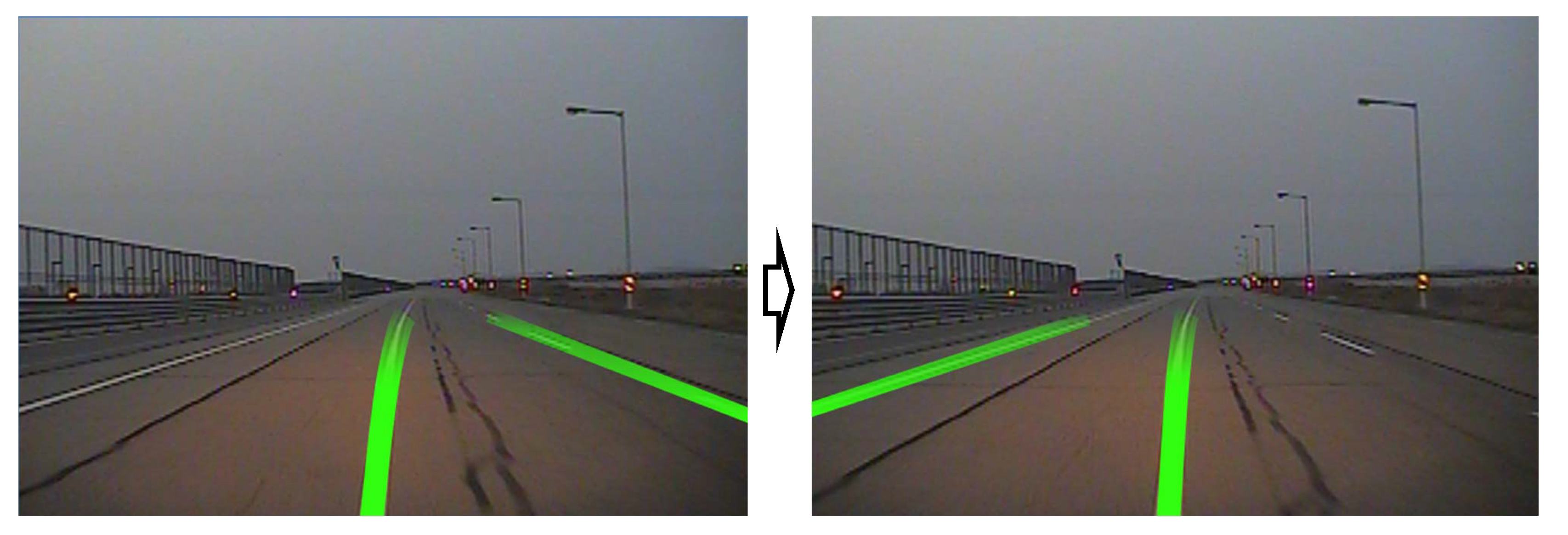
Meanwhile, for lane change, the autonomous vehicle tracks the desired lateral offset that increases or decreases the lateral offset error from the original lane, while the front camera obtains the original lane information. In this situation, the vehicle crosses over between the original and target lanes for lane change, and the camera vision sensor starts obtaining the target lane information instead of that of the original lane. Consequently, an inevitable jumped lane information is obtained as shown in Figure 1. This discrete change in lane information, i.e., the state jump, may deteriorate the lateral control performance. Moreover, the ALCS can cause serious accidents because of sudden changes in the control input. Thus, these discrete changes in the lane information should be considered while implementing the ALCS.

To overcome the state jump problem, adding and subtracting the lane width might be a solution at the moment the vehicle changes the lane. However, it is dangerous if the detection time of the camera vision sensor and the calculation time of the system are different when the vehicle is controlled for the lane change because of the unmatched state information, as shown in Figure 1. This figure shows that a sudden control input is generated becuase of the unmatched state information with respect to time in our real-vehicle experiment. The reason is that the camera vision sensor usually has a hysteresis to reduce the detection error when driving near the lane. Therefore, it is difficult to detect a state jump and provide the control system with synchronized lane change information.

In this study, we proposed a linear parameter varying (LPV) lateral motion controller using the cylinder domain to overcome the state jump problem.

First, the lateral motion of vehicle dynamics in a plane is reformulated in the cylinder domain. Gluing the edges of the plane road creates the cylindrical domain. Further, the state jump does not occur due to a lane change in this cylinder domain means that the vehicle come back to the original position by maintaining its continuous state.

Second, to solve the nonlinear term caused by domain gluing, the procedure of the LPV design method is proposed. The lateral movement of the vehicle in the new cylinder domain is nonlinear; however, the proposed method allows the designing of linear controllers without considering complicated nonlinear controllers. By considering the nonlinear bounded varying term as a system parameter using the trigonometric function constraint, the overall control design procedure changes into linear parameter dependent gain-scheduling problem.

To the best of our knowledge, the proposed method is the first algorithm in literature to avoid state jump during lane changes as applicable to the automotive industry. The contributions of this study can be summarized as follows:

• A new lateral motion model for a lane change system is introduced in the cylinder domain. In addition, the overall lateral motion controller design procedure for autonomous lane change system is presented in the cylinder domain.
• State jump in lateral offset does not appear in the proposed cylinder domain due to its gluing characteristics. Consequently, the proposed method does not need to consider the lane crossing time when developing a lane change controller. Using simple sine and cosine references, the vehicle can complete the lane change process effectively.
• The LPV controller makes it possible to control the vehicle using simple linear controller, and has a significant advantage in the computation time for low-cost electronic control unit (ECU). It is validated with the MATLAB/Simulink including the vehicle dynamics analysis program CarSim. Using the sub-optimal gain calculated from both pre-calculated optimal gain and interpolation from updated varying parameter, the proposed method exhibits reasonable performance in lane change.

1.1. Vehicle Lateral Motion Model

• Nomenclature:

  -

  y: distance from the center of gravity (c.g.) to the center of turn in ${}^v\left\{xyz\right\}$;

  -

  $y_{des}$: distance from the lane center to the center of turn in ${}^v\left\{xyz\right\}$;

  -

  $e_y=y-y_{des}$: lateral lane center offset at c.g.;

  -

  L: look-ahead distance;

  -

  ${\psi }_{des}$: yaw angle slope of the lane center;

  -

  $e_{\psi }={\psi }_{des}-\psi$: heading angle error at c.g.;

  -

  $\dot{\psi }$: yaw rate;

  -

  V: velocity of the vehicle at c.g.;

  -

  $\alpha$: tire slip angle;

  -

  $\beta$: side slip angle at c.g.;

  -

  $C_{\alpha }$: cornering stiffness of the tire;

  -

  $F_y$: lateral tire force;

  -

  $I_z$: yaw inertia of the vehicle;

  -

  $M_z$: moment balance of the vehicle;

  -

  m: total mass of the vehicle;

  -

  l: distance of the tire from c.g. of the vehicle;

  -

  u: input (=$\delta$: steer angle) of the control system.

• Subscripts:

  -

  f: front;

  -

  r: rear;

  -

  x: longitudinal;

  -

  y: lateral;

  -

  $des$: desired.

We introduce the generally used vehicle model in terms of lateral position and heading errors with respect to the road for lateral control to regulate both lateral position and heading errors. This implies that the vehicle is maintained at the road center. Further, we derive the new vehicle motion model for lateral control systems by considering the jumped state of the lateral offset in a lane-change situation. The new model presents the plane motion of the vehicle in the cylinder domain.

1.2. Lateral Motion Model in Plane Domain

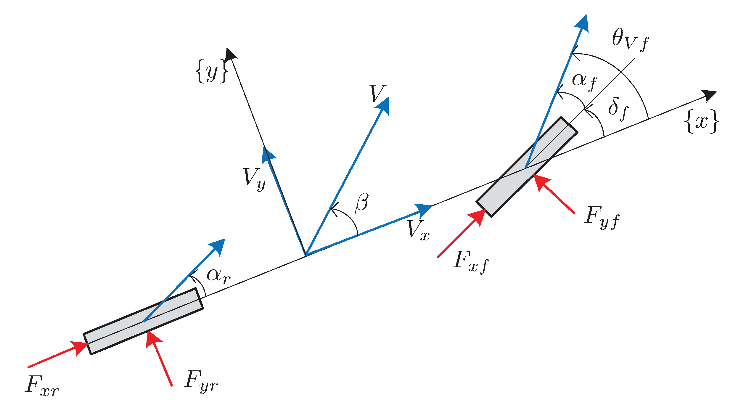
In this study, a generalized lateral dynamic motion model of a vehicle is considered. The lateral dynamics of the bicycle model as shown in Figure 2 are described by summing the forces $F_y$ and moment $M_z$ at the center of gravity of the vehicle:

$$\begin{array}{cc}\hfill \sum F_y& =F_{yf}+F_{yr}=m(\ddot{y}+\dot{\psi }{V}_x)\hfill \\ \hfill \sum M_z& =l_f{F}_{yf}+l_r{F}_{yr}=I_z\ddot{\psi }.\hfill \end{array}$$

(1)

For small slip angles, the lateral tire force $F_y$ can be approximated as a linear function of the tire slip angle (${\alpha }_f,{\alpha }_r$) [16,17]. The tire slip angle is defined as the angle between the orientation of the tire and that of the velocity vector of the wheel ${\theta }_V$:

$$\begin{array}{cc}\hfill F_{yf}& =2C_{\alpha f}{\alpha }_f=2C_{\alpha f}(\delta -{\theta }_{V_f})\hfill \\ \hfill F_{yr}& =2C_{\alpha r}{\alpha }_r=2C_{\alpha r}(-{\theta }_{V_r}),\hfill \end{array}$$

(2)

where $C_{\alpha }$ denotes tire cornering stiffness. Using small angle approximations for both ${\theta }_{V_f}$ and ${\theta }_{V_r}$, we obtain

$$\begin{array}{c}\hfill {\displaystyle {\theta }_{V_f}=\frac{\dot{y}+l_f\dot{\psi }}{V_x}=\frac{-V_y+l_f\dot{\psi }}{V_x}=-\beta +\frac{l_f\dot{\psi }}{V_x},}\\ \hfill {\displaystyle {\theta }_{V_r}=\frac{\dot{y}-l_r\dot{\psi }}{V_x}=\frac{-V_y-l_r\dot{\psi }}{V_x}=-\beta -\frac{l_r\dot{\psi }}{V_x},}\end{array}$$

(3)

with

$$\begin{array}{c}\hfill \beta \approx tan\left(\beta \right)=\frac{V_y}{V_x}.\end{array}$$

(4)

For the LKS, we define the following two state variables:

• $e_y$ is the lateral offset error at the center of gravity of the vehicle from the lane center.
• $e_{\psi }$ denotes the heading error of the vehicle with respect to the desired road.

Then, the dynamic model for the lateral control system can be described as follows in terms of state vector $\mathbf{x}={\left[\begin{array}{cccc}{e}_y& {\dot{e}}_y& e_{\psi }& {\dot{e}}_{\psi }\end{array}\right]}^T$, control input $u=\delta$, and external signal $\phi ={\left[\begin{array}{c}{\dot{\psi }}_{des}\end{array}\right]}^T$ [12,16,18]:

$$\begin{array}{cc}\hfill \dot{\mathbf{x}}& =A\mathbf{x}+Bu+B_{\phi }\phi \hfill \end{array}$$

(5)

where,

$$\begin{array}{c}\hfill A=\left[\begin{array}{cccc}0& 1& 0& 0\\ 0& a_{22}& a_{23}& a_{24}\\ 0& 0& 0& 1\\ 0& a_{42}& a_{43}& a_{44}\end{array}\right],B=\left[\begin{array}{c}0\\ b_{21}\\ 0\\ b_{41}\end{array}\right],B_{\phi }=\left[\begin{array}{c}0\\ a_{24}-V_x\\ 0\\ a_{44}\end{array}\right]\end{array}$$

with

$${\displaystyle a_{22}=-\frac{2(C_{\alpha f}+C_{\alpha r})}{m{V}_x},a_{23}=-a_{22}{V}_x,}$$

$${\displaystyle a_{24}=-\frac{2(C_{\alpha f}{l}_f-C_{\alpha r}{l}_r)}{m{V}_x^2},a_{42}=-\frac{2(C_{\alpha f}{l}_f-C_{\alpha r}{l}_r)}{I_z},}$$

$${\displaystyle a_{43}=-a_{42},a_{44}=-\frac{2(C_{\alpha f}{l}_f^2+C_{\alpha r}{l}_r^2)}{I_z{V}_x},}$$

$${\displaystyle b_{21}=\frac{2C_{\alpha f}}{m{V}_x},b_{41}=\frac{2C_{\alpha f}{l}_f}{I_z}.}$$

Equation (5) represents the lateral motion of the vehicle with respect to the road in the plane domain. $e_y$, $e_{\psi }$, and ${\dot{e}}_{\psi }$ can be obtained using the camera sensor [11].

Remark 1.

The lateral offset, $e_y$, is measured based on the current driving lane. When the vehicle changes the lane, $e_y$ increases gradually until the vehicle crosses the lane. After the vehicle crosses the lane, a jump of $e_y$ occurs because of the change of driving lane, and the error decreases gradually. In other words, the sign of the lateral offset suddenly changes during lane change in the plane motion model when the camera vision sensor begin obtaining the target lane information instead of the information of the original lane. That is, the lateral offset jumps during lane change. To overcome these problems in the plane motion model, we propose the cylinder domain approach, which can remove state jumps in the lateral offset.

1.3. Lateral Motion Model in Cylinder Domain

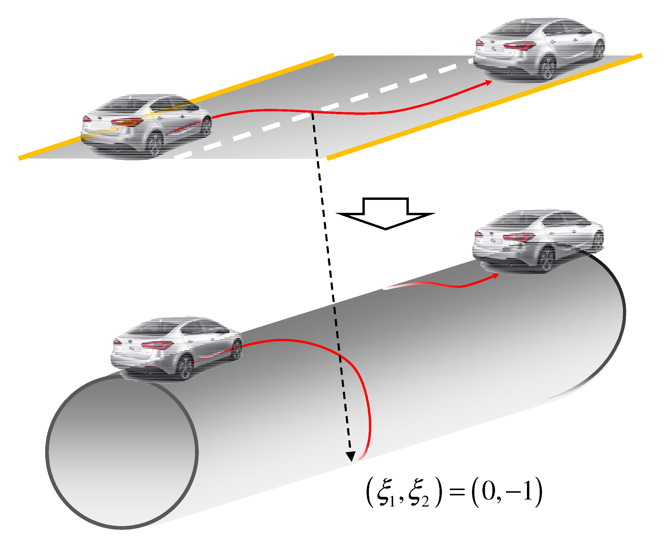
The main objective behind removing the state jump is to develop a lateral motion model in the cylinder domain. When the vehicle changes lanes, the reference lane for the travelling car changes to another lane. To eliminate this phenomenon, we glue the sides of the plane road to construct a cylindrical domain. Let us consider the lane change situation on a two lane road, as shown in Figure 3.

As shown in Figure 3, each lane is transformed into one half of a cylindrical surface by gluing the edges of the plane domain. The initial position of the vehicle is at the top of the cylinder. Further, the vehicle is positioned at the bottom of the cylinder when it crosses the lane, and at the top of the cylinder when the lane change is completed. Consequently, there is no change of sign in the lateral offset; however, the vehicle motion should be analyzed in the new domain accordingly.

To describe the vehicle motion model in the cylinder domain, let us now define the new states ${\xi }_i$ using ${\left[\begin{array}{cccc}{e}_y& {\dot{e}}_y& e_{\psi }& {\dot{e}}_{\psi }\end{array}\right]}^T={\left[\begin{array}{cccc}{x}_1& x_2& x_3& x_4\end{array}\right]}^T$ as follows:

$$\begin{array}{cc}\hfill {\xi }_1& =sin\left({\displaystyle \frac{2\pi }{L_w}{x}_1}\right),\hfill \\ \hfill {\xi }_2& =cos\left({\displaystyle \frac{2\pi }{L_w}{x}_1}\right),\hfill \\ \hfill {\xi }_3& =x_2,\hfill \\ \hfill {\xi }_4& =x_3,\hfill \\ \hfill {\xi }_5& =x_4\hfill \end{array}$$

(6)

where $L_w$ denotes the road lane width which is obtained using a vision sensor and generally considered as a constant value.

Now, the 2D motion of the vehicle changes in 3D motion by satisfying the following constraint:

$$\begin{array}{c}\hfill {\xi }_1^2+{\xi }_2^2={sin}^2\left({\displaystyle \frac{2\pi }{L_w}{x}_1}\right)+{cos}^2\left({\displaystyle \frac{2\pi }{L_w}{x}_1}\right)=1.\end{array}$$

(7)

In other words, the vehicle travels along the surface of the cylinder whose cross section is in the shape of a unit circle. Further, we can obtain the dynamics of ${\xi }_1$ and ${\xi }_2$ with constant velocity from (5) and (6) as:

$$\begin{array}{cc}\hfill {\dot{\xi }}_1& {\displaystyle =\frac{2\pi }{L_w}{\dot{x}}_{1}cos\left({\displaystyle \frac{2\pi }{L_w}{x}_1}\right),}\hfill \\ \hfill {\dot{\xi }}_2& {\displaystyle =-\frac{2\pi }{L_w}{\dot{x}}_{1}sin\left({\displaystyle \frac{2\pi }{L_w}{x}_1}\right).}\hfill \end{array}$$

(8)

Furthermore, the overall vehicle dynamics of lateral motion with respect to the road is represented in terms of state vector ${\left[\begin{array}{ccccc}{\xi }_1& {\xi }_2& {\xi }_3& {\xi }_4& {\xi }_5\end{array}\right]}^T$, control input u and external signal $\phi$ as follows:

Remark 2.

For the LKS, the vehicle should maintain its driving lane while satisfying the lateral offset $e_y=0$. Therefore, in the proposed cylinder domain, the desired values of ${\xi }_1$ and ${\xi }_2$ for LKS are 0 and 1, respectively.

$$\dot{\xi }=f\left(\xi ,u,\phi \right)$$

(9)

with

$$\begin{array}{cc}\hfill {\dot{\xi }}_1& {\displaystyle =\frac{2\pi }{L_w}{\xi }_3{\xi }_2}\hfill \\ \hfill {\dot{\xi }}_2& {\displaystyle =-\frac{2\pi }{L_w}{\xi }_3{\xi }_1}\hfill \\ \hfill {\dot{\xi }}_3& =a_{22}{\xi }_3+a_{23}{\xi }_4+a_{24}{\xi }_5+b_{21}u+(a_{24}-V_x)\phi \hfill \\ \hfill {\dot{\xi }}_4& ={\xi }_5\hfill \\ \hfill {\dot{\xi }}_5& =a_{42}{\xi }_3+a_{43}{\xi }_4+a_{44}{\xi }_5+b_{41}u+a_{44}\phi ,\hfill \\ \hfill y& ={\left[\begin{array}{cccc}{\xi }_1& {\xi }_2& {\xi }_4& {\xi }_5\end{array}\right]}^T.\hfill \end{array}$$

In (9), both vehicle states ${\xi }_1$ and ${\xi }_2$ are available because $x_1$ is measured using the vision sensor. In addition, $x_3$ is also obtained using the vision sensor and $x_4$ from the in-vehicle sensor.

The gluing function $\rho \left(x\right)$ and its inverse, which transform system (5) into (9), are described as follows:

$$\begin{array}{cc}\hfill \xi :=\rho \left(x\right)& =\left[\begin{array}{c}sin\left({\displaystyle \frac{2\pi }{L_w}{x}_1}\right)\\ cos\left({\displaystyle \frac{2\pi }{L_w}{x}_1}\right)\\ x_2\\ x_3\\ x_4\end{array}\right],\hfill \\ \hfill {\rho }^{-1}\left(\xi \right)& =\left[\begin{array}{c}{\displaystyle \overline{\mathrm{sgn}}\left({sin}^{-1}\left({\xi }_1\right)\right)\frac{L_w}{2\pi }{cos}^{-1}\left({\xi }_2\right)}\\ {\xi }_3\\ {\xi }_4\\ {\xi }_5\end{array}\right].\hfill \end{array}$$

(10)

Using Equation (10), one can obtain the original state $x_i$ of lateral dynamics.

Remark 3.

In the cylinder domain, the vehicle position can be represented as ${\left\{x,{\xi }_1,{\xi }_2\right\}}^l$ rather than ${\left\{x,y\right\}}^l$, where the superscript l denotes the local coordinate of vehicle. When the vehicle changes the lane, the trajectory of vehicle changes as follows:

• Driving on the current lane center ${\left\{x_{t_1},0,1\right\}}^l$
• The moment the vehicle crosses the lane ${\left\{x_{t_2},0,-1\right\}}^l$
• Driving on the target lane center ${\left\{x_{t_3},0,1\right\}}^l$

where $x_{t_i}$ denotes the longitudinal position at time $t_i$. As compared to the lateral model (5) in the plane domain, the lateral offset jump does not occur during the lane change in the cylinder domain lateral model (9).

Designing the trajectory of a vehicle for lane change is simple in cylinder domain. Let us consider the lane change to the right. The lateral offset with respect to the road increases until half of the lane width. After the moment of crossing the lane, the lateral offset decreases to zero. Further, using Equation (10), one can obtain the following reference trajectory for the autonomous lane change system.

$$\begin{array}{c}\hfill {\xi }_1^r\left(t\right),{\xi }_2^r\left(t\right):\left\{\begin{array}{cc}\mathrm{RLC}\hfill & =sin\left({\displaystyle \frac{2\pi t}{t_{lc}}}\right),cos\left({\displaystyle \frac{2\pi t}{t_{lc}}}\right),\hfill \\ \hfill \mathrm{LLC}& =-sin\left({\displaystyle \frac{2\pi t}{t_{lc}}}\right),cos\left({\displaystyle \frac{2\pi t}{t_{lc}}}\right),\hfill \end{array}\right.\end{array}$$

(11)

where RLC and LLC denote right and left lane changes, respectively. The desired lane change time $t_{lc}$ is a user-defined parameter for the lane change system. In the simulation section, we can see the example of reference trajectories.

2. Controller Design in Cylinder Domain

In this section, we describe the development of the LPV controller in the cylinder domain. We propose a linear controller that can effectively reflect the geometrical aspects of the newly presented cylinder domain. Thus, the lateral motion model in the cylinder domain is linearized; however, it is designed to reflect the nonlinearity as much as possible. To achieve the above objectives, two proposed methods (parameterization of nonlinearly changing variables and definition of auxiliary variable for linearization) are described in this session.

2.1. Development of LPV System

We can change the nonlinear dynamics into linear dynamics by considering the nonlinear bounded terms in the model as matrix coefficients. The ${\xi }_1$ and ${\xi }_2$ states in (10) are nonlinear for the original state $x_1$. Therefore, we define these two variables as the varying parameter as $\theta (x_1,L_w)={\left[\begin{array}{cc}{\theta }_1(x_1,L_w)& {\theta }_2(x_1,L_w)\end{array}\right]}^T$:

$$\begin{array}{cc}\hfill {\theta }_1(x_1,L_w)& ={\xi }_2,\hfill \\ \hfill {\theta }_2(x_1,L_w)& =-{\xi }_1,\hfill \end{array}$$

(12)

where $x_1$ and $L_w$ are available from the vision sensor. Now, the first two equations in (9) can be represented as follows:

$$\begin{array}{cc}\hfill {\dot{\xi }}_1& {\displaystyle =\frac{2\pi }{L_w}{\xi }_3{\xi }_2=\frac{2\pi }{L_w}{\theta }_1{\xi }_3,}\hfill \\ \hfill {\dot{\xi }}_2& {\displaystyle =-\frac{2\pi }{L_w}{\xi }_3{\xi }_1=\frac{2\pi }{L_w}{\theta }_2{\xi }_3.}\hfill \end{array}$$

(13)

Note that the lateral offset error $x_1$ is unbounded, and the lane width $L_w$ is not zero on a highway. Nevertheless, the varying parameters are bounded because of the trigonometric function.

$$\begin{array}{cc}\hfill {\theta }_1(x_1,L_w)& \in \left[\begin{array}{cc}{\overline{\theta }}_1& {\underline{\theta }}_1\end{array}\right],\hfill \\ \hfill {\theta }_2(x_1,L_w)& \in \left[\begin{array}{cc}{\overline{\theta }}_2& {\underline{\theta }}_2\end{array}\right].\hfill \end{array}$$

(14)

Now, we introduce a small auxiliary variable for the non-linearized term between ${\xi }_{1,2}$ and ${\xi }_3$. In practice, ${\xi }_1$ and ${\xi }_2$ are approximately accurate because their values are calculated by the measured signal from lateral offset and width of lane. However, ${\xi }_3$ contains uncertainty because it is obtained from an estimator or numerical derivation of the lateral offset. Therefore, we introduce auxiliary variables $\sigma$ to ${\xi }_3$ rather than ${\xi }_1$ and ${\xi }_2$. Let us define an auxiliary variable $\sigma$ that reflects the nonlinearized term between ${\xi }_{1,2}$ and ${\xi }_3$ as follows:

$$\begin{array}{cc}\hfill {\dot{\xi }}_1& {\displaystyle \simeq \frac{2\pi }{L_w}\left({\xi }_3+\sigma \right){\xi }_2,}\hfill \\ \hfill {\dot{\xi }}_2& {\displaystyle \simeq -\frac{2\pi }{L_w}\left({\xi }_3+\sigma \right){\xi }_1.}\hfill \end{array}$$

(15)

Further, the linearized Equation (14) can be reformulated as follows using Equation (15):

$$\begin{array}{cc}\hfill {\dot{\xi }}_1& {\displaystyle \simeq \frac{2\pi }{L_w}\left({\xi }_3+\sigma \right){\xi }_2}\hfill \\ \hfill & {\displaystyle =\frac{2\pi }{L_w}{\xi }_3{\xi }_2+\frac{2\pi }{L_w}\sigma {\xi }_2}\hfill \\ \hfill & {\displaystyle =\frac{2\pi }{L_w}{\theta }_1{\xi }_3+\epsilon {\xi }_2}\hfill \end{array}$$

(16)

The same can be applied for ${\dot{\xi }}_2$.

Therefore, the nonlinear dynamics (9) with the cylinder domain can be interpreted as a form of the LPV system with variation of lateral offset and lane width. Both parameterizing the nonlinear bounded varying parameter (12) and defining the auxiliary variable (15), result in the following LPV system:

$$\begin{array}{cc}\hfill \dot{\xi }& =A_{\xi }\left(\theta \right)\xi +B_{\xi }u+B_{\xi ,\phi }\phi ,\hfill \end{array}$$

(17)

where

$$\begin{array}{cc}\hfill A_{\xi }\left(\theta \right)& =\left[\begin{array}{ccccc}0& \sigma & \frac{2\pi }{L_w}{\theta }_1& 0& 0\\ -\sigma & 0& \frac{2\pi }{L_w}{\theta }_2& 0& 0\\ 0& 0& a_{22}& a_{23}& a_{24}\\ 0& 0& 0& 0& 1\\ 0& 0& a_{42}& a_{43}& a_{44}\end{array}\right],\hfill \\ \hfill B_{\xi }& ={\left[\begin{array}{cc}0& B\end{array}\right]}^T,B_{\xi ,\phi }={\left[\begin{array}{cc}0& B_{\phi }\end{array}\right]}^T.\hfill \end{array}$$

By introducing auxiliary variable we can obtain both a reflection of the non-linearized term and controllability of the given system.

2.2. Interpolation Based Gain-Scheduling

Now, we choose the following vertex $\mathbf{V}$ among the several candidates by considering a bound of the time-varying parameter:

$$\begin{array}{c}\hfill \mathbf{V}=\left[\begin{array}{cccc}{v}_1& v_2& v_3& v_4\end{array}\right]=\left[\begin{array}{cccc}{\underline{\theta }}_1& 0& {\overline{\theta }}_1& 0\\ 0& {\underline{\theta }}_2& 0& {\overline{\theta }}_2\end{array}\right].\end{array}$$

(18)

Then, the varying parameter vector, $\theta \in {\mathbb{R}}^2$ is rewritten in the following polytopic form

$$\begin{array}{cc}\hfill \theta (x_1,L_w)& =\mathbf{V}\mathit{\eta }\left(\theta \right)\hfill \end{array}$$

(19)

where $\mathit{\eta }\left(\theta \right)={\left[\begin{array}{cccc}{\eta }_1\left(\theta \right)& {\eta }_2\left(\theta \right)& {\eta }_3\left(\theta \right)& {\eta }_4\left(\theta \right)\end{array}\right]}^T\in {\mathbb{R}}^4$, ${\eta }_i\ge 0,{\sum }_{i=1}^4{\eta }_i\left(\theta \right)=1$, is the convex interpolation parameter vector.

Note that the convex interpolation parameter vector $\xi \left(\theta \right)$ is uniquely determined by the given time-varying parameter vector $\theta$ if the vertex $\mathbf{V}$ is invertible in (19). However, the given vertex in (18) is not invertible and one cannot determine the interpolation parameter vector. Therefore, we introduce the internal division constraints to make the given vertex invertible. The defined varying parameters satisfy the trigonometric constraints; thus, the parameters always exist on the surface of the cylinder as follows:

$$\begin{array}{c}\hfill {\theta }_1^2+{\theta }_2^2={cos}^2\left({\displaystyle \frac{2\pi }{L_w}{x}_1}\right)+{sin}^2\left({\displaystyle \frac{2\pi }{L_w}{x}_1}\right)=1.\end{array}$$

(20)

Furthermore, the ranges of the vertices are equal in a 2D space. Considering the same range of varying parameter and ${\sum }_{i=1}^4{\eta }_i\left(\theta \right)=1$ lead to the following equation:

$${\eta }_1\left(\theta \right)+{\eta }_3\left(\theta \right)={\eta }_2\left(\theta \right)+{\eta }_4\left(\theta \right)=0.5.$$

(21)

In addition, ${\theta }_1$ is the internal division of ${\overline{\theta }}_1$ and ${\underline{\theta }}_1$ by ${\eta }_1$ and ${\eta }_3$. Thus, the varying parameter can be represented as follows:

$$\begin{array}{cc}\hfill {\theta }_1& {\displaystyle =\frac{{\eta }_1{\underline{\theta }}_1+{\eta }_3{\overline{\theta }}_1}{{\eta }_1+{\eta }_3}}\hfill \\ \hfill & ={\eta }_{1}2{\underline{\theta }}_1+{\eta }_{3}2{\overline{\theta }}_1.\hfill \end{array}$$

(22)

We can also obtain the equation of ${\theta }_2$ as ${\theta }_2={\eta }_{2}2{\underline{\theta }}_2+{\eta }_{4}2{\overline{\theta }}_2$.

As a result, constraints (21) and (22) give the following expanded vertices matrix $\widehat{\mathbf{V}}$ and the expanded parameter vector $\widehat{\Theta }$ can be defined as follows:

$$\begin{array}{cc}\hfill \widehat{\mathbf{V}}& =\left[\begin{array}{c}2\mathbf{V}\\ M^{2\times 4}\end{array}\right]=\left[\begin{array}{cccc}2{\underline{\theta }}_1& 0& 2{\overline{\theta }}_1& 0\\ 0& 2{\underline{\theta }}_2& 0& 2{\overline{\theta }}_2\\ 1& 0& 1& 0\\ 0& 1& 0& 1\end{array}\right],\hfill \\ \hfill \widehat{\Theta }& =\left[\begin{array}{c}\Theta \\ s^{2\times 1}\end{array}\right]={\left[\begin{array}{cccc}{\theta }_1& {\theta }_2& 0.5& 0.5\end{array}\right]}^T,\hfill \end{array}$$

(23)

where $M\in {\mathbb{R}}^{2\times 4}$ is the expanded matrix for $\widehat{\mathbf{V}}$, and $s\in {\mathbb{R}}^2$ is the expanded vector for $\widehat{\Theta }$. Now, the vertex in (23) is invertible and the convex interpolation parameter is uniquely determined as $\eta \left(\theta \right)={\widehat{\mathbf{V}}}^{-1}\widehat{\Theta }$.

Using the convex interpolation parameters, ${\eta }_i\left(\theta \right)$, one can represent the system matrix as the following parameter-dependent matrix $A_{\xi }\left(\theta \right)$:

$$\begin{array}{c}\hfill A_{\xi }\left(\theta \right)={\displaystyle \sum _{i=1}^4}{\eta }_i\left(\theta \right)A_{\xi }^{\left(i\right)},\end{array}$$

(24)

where

$$\begin{array}{cc}\hfill A_{\xi }^{\left(1\right)}& =A_{\xi }\left(0\right)+{\underline{\theta }}_1{\widehat{A}}_{\xi }^{\left(1\right)},\hfill \\ \hfill A_{\xi }^{\left(2\right)}& =A_{\xi }\left(0\right)+{\underline{\theta }}_2{\widehat{A}}_{\xi }^{\left(2\right)},\hfill \\ \hfill A_{\xi }^{\left(3\right)}& =A_{\xi }\left(0\right)+{\overline{\theta }}_1{\widehat{A}}_{\xi }^{\left(1\right)},\hfill \\ \hfill A_{\xi }^{\left(4\right)}& =A_{\xi }\left(0\right)+{\overline{\theta }}_2{\widehat{A}}_{\xi }^{\left(2\right)},\hfill \end{array}$$

(25)

with

$$\begin{array}{cc}\hfill A_{\xi }\left(0\right)& =\left[\begin{array}{ccccc}0& \sigma & 0& 0& 0\\ -\sigma & 0& 0& 0& 0\\ 0& 0& a_{22}& a_{23}& a_{24}\\ 0& 0& 0& 0& 1\\ 0& 0& a_{42}& a_{43}& a_{44}\end{array}\right],\hfill \\ \hfill {\widehat{A}}_{\xi }^{\left(1\right)}& =\left[\begin{array}{ccc}{\mathbf{0}}_{1\times 2}& \frac{2\pi }{L_w}{\theta }_1& {\mathbf{0}}_{1\times 2}\\ {\mathbf{0}}_{1\times 2}& 0& {\mathbf{0}}_{1\times 2}\\ & {\mathbf{0}}_{3\times 5}\end{array}\right],{\widehat{A}}_{\xi }^{\left(2\right)}=\left[\begin{array}{ccc}{\mathbf{0}}_{1\times 2}& 0& {\mathbf{0}}_{1\times 2}\\ {\mathbf{0}}_{1\times 2}& \frac{2\pi }{L_w}{\theta }_2& {\mathbf{0}}_{1\times 2}\\ & {\mathbf{0}}_{3\times 5}\end{array}\right].\hfill \end{array}$$

Here, ${\widehat{A}}_{\xi }^{\left(j\right)}$ are the real fixed nodal matrices associated with $\theta (x_1,L_w)={\left[\begin{array}{cc}{\theta }_1& {\theta }_2\end{array}\right]}^T$.

Now, a gain-scheduled optimal control gain $K\left(\theta \right)$ will be considered using convex interpolation. As the control problem for vehicle lateral motion is reformulated for the LPV systems, we can design a linear controller. In this study, the process of LPV controller design is proposed in the cylinder domain, so the validity is verified through the basic linear quadratic (LQ) controller for reference tracking.

We can pre-calculate the optimal gain $K^{\left(i\right)}$ for each vertex $A^{\left(i\right)}$ from the well-known Riccati equation. As we mentioned before, once the varying parameter is updated, the convex interpolation parameter is uniquely determined as $\eta \left(\theta \right)={\widehat{\mathbf{V}}}^{-1}\widehat{\Theta }$ using the Equation (23). From the measured varying parameters, we can calculate and update the sub-obtimal gain for the lateral motion controller as follows [19,20]:

$$\begin{array}{c}\hfill K\left(\theta \right)={\displaystyle \sum _{i=1}^4}{\eta }_i\left(\theta \right)K^{\left(i\right)}.\end{array}$$

(26)

Note that the gain is not optimal but sub-optimal because the proposed method uses simple interpolation from each vertex. Nevertheless, the proposed method exhibits reasonable performance with a small amount of computation, which can be confirmed by the simulation results in the next section.

3. Simulation Results

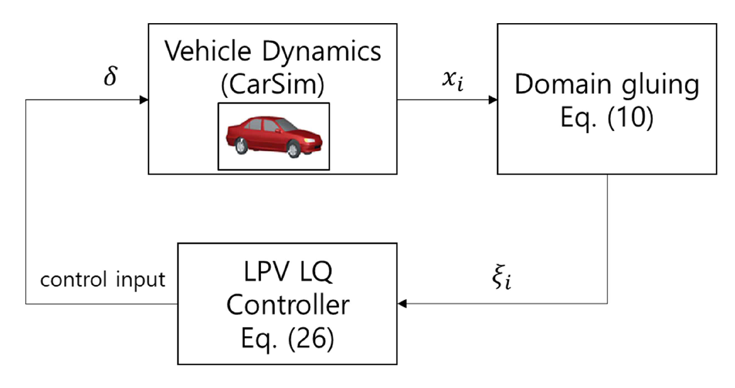
The proposed algorithm is designed and validated via MATLAB/Simulink. A C-class hatchback model in CarSim from Mechanical Simulation is also used to solve the vehicle dynamics. From the vision sensor in the CarSim, one can obtain the state of vehicle such as lateral offset and heading offset with respect to the road. The overall simulation-in-the-loop architecture of the proposed ALCS is shown in Figure 4.

Two lane change scenarios are considered in this study for the validation:

• Formal sine and cosine trajectory-based lane change to the right within 5 s;
• Human driver trajectory-based lane change to the left within 3 s.

One of the basic methods of changing lanes is by setting a reference using sine and cosine components, as presented in this study. However, the reference that appears when a human driver changes lanes does not perfectly follow sine and cosine [21]. Therefore, the second scenario is conducted to verify the proposed algorithm under a non-sinusoidal reference trajectory.

In both cases, the vehicle travels a straight lane at 60 km/h. The nominal parameters of a C-class hatchback in CarSim are used for the proposed ALCS.

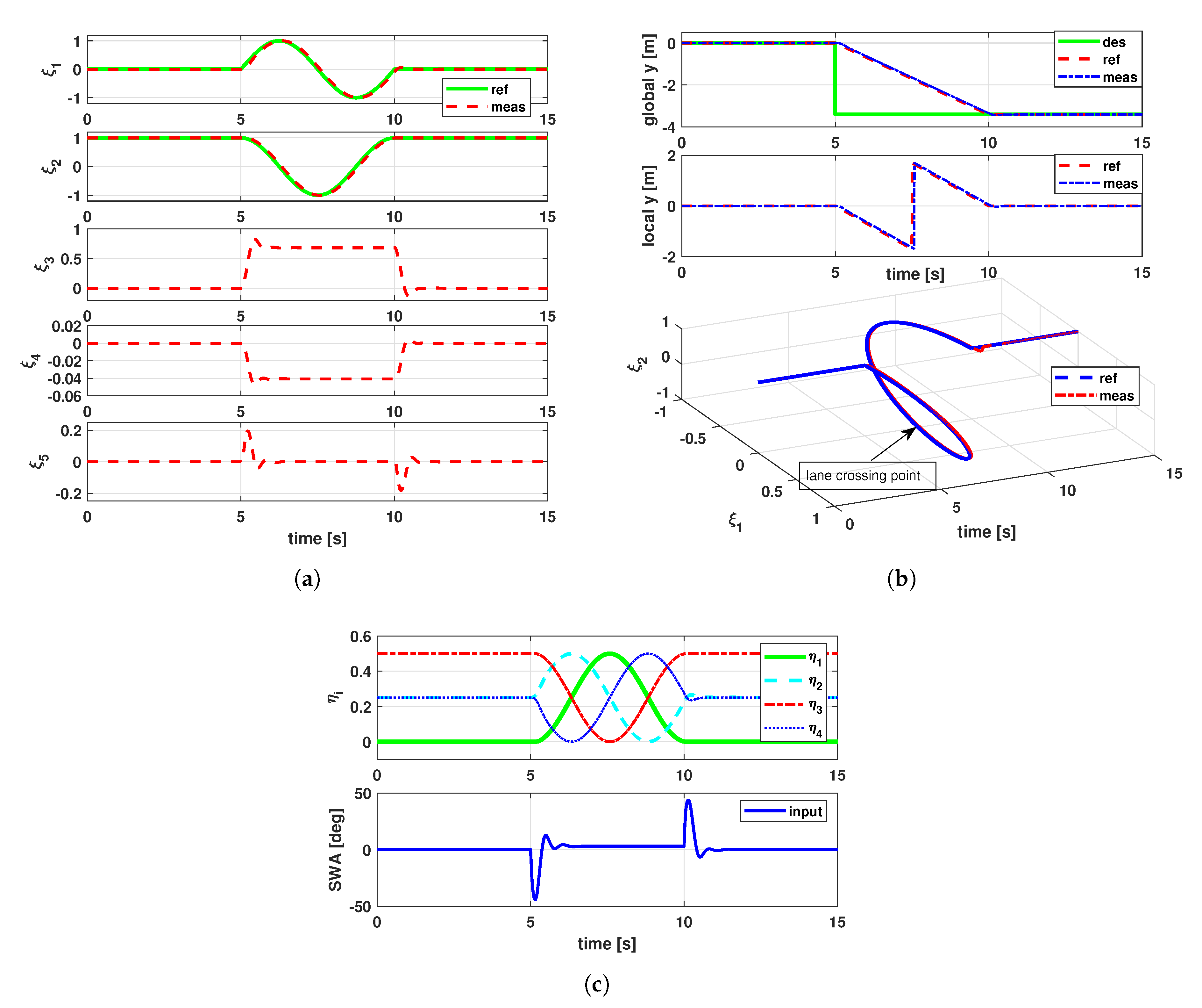
3.1. Scenario 1: Sine and Cosine Based Trajectory

In scenario 1, the vehicle started changing lanes at 5 s to the right during 5 s. Figure 5a shows the reference trajectory and measured state in cylinder domain. One can observe that to change the lane to the right, the reference trajectories of ${\xi }_1$ and ${\xi }_2$ are designed using $sin(2\pi t/5)$ and $cos(2\pi t/5)$. The derivative of the reference is not continuous at 5 s and 10 s; thus, it can be seen that the output value of the controller is instantaneously large in Figure 5c. Therefore, it can be seen in Figure 5a that error of yaw rate, ${\xi }_5$, also shows a similar pattern. The rate of lateral offset, ${\xi }_3$, starts to increase at 5 s and has a constant value which means a constant lateral acceleration during lane change, and then decreases to zero at the end of lane change at 10 s.

Trajectories of the vehicle in the global, local, and cylinder domains are shown in Figure 5b, respectively. The right lane change means the desired lateral position of vehicle is changed as −3.4 m in the global coordinate, as plotted with the green line. Thus, we designed the reference trajectories ${\xi }_1$ and ${\xi }_2$ as shown in Figure 5a to change to the right lane. At the start of lane change, the trajectory of the vehicle state exists on the original position $\left({\xi }_1,{\xi }_2\right)=(0,1)$. Further, the trajectory of the vehicle state returns to the original position at the end of lane change past the lane crossing point (0, −1), as described in the cylinder domain.

We can see the lateral offset in local coordinate jumps when the vehicle cross the lane at about 7.5 s. The designed trajectories can be plotted in local coordinates using the inverse of the gluing function in (10), as plotted with the red dashed line. However, both reference trajectory and measured state do not have jump state in the cylinder domain. In other words, even if the reference trajectory is generated in the cylinder domain and the control method is applied, the movement of the vehicle is the same as that on the plane.

The convex interpolation parameters for the LPV controller are shown in Figure 5c. As the nonlinear varying parameter $\theta$ changes, the corresponding interpolation parameters change in a similar manner as the sine and cosine forms.

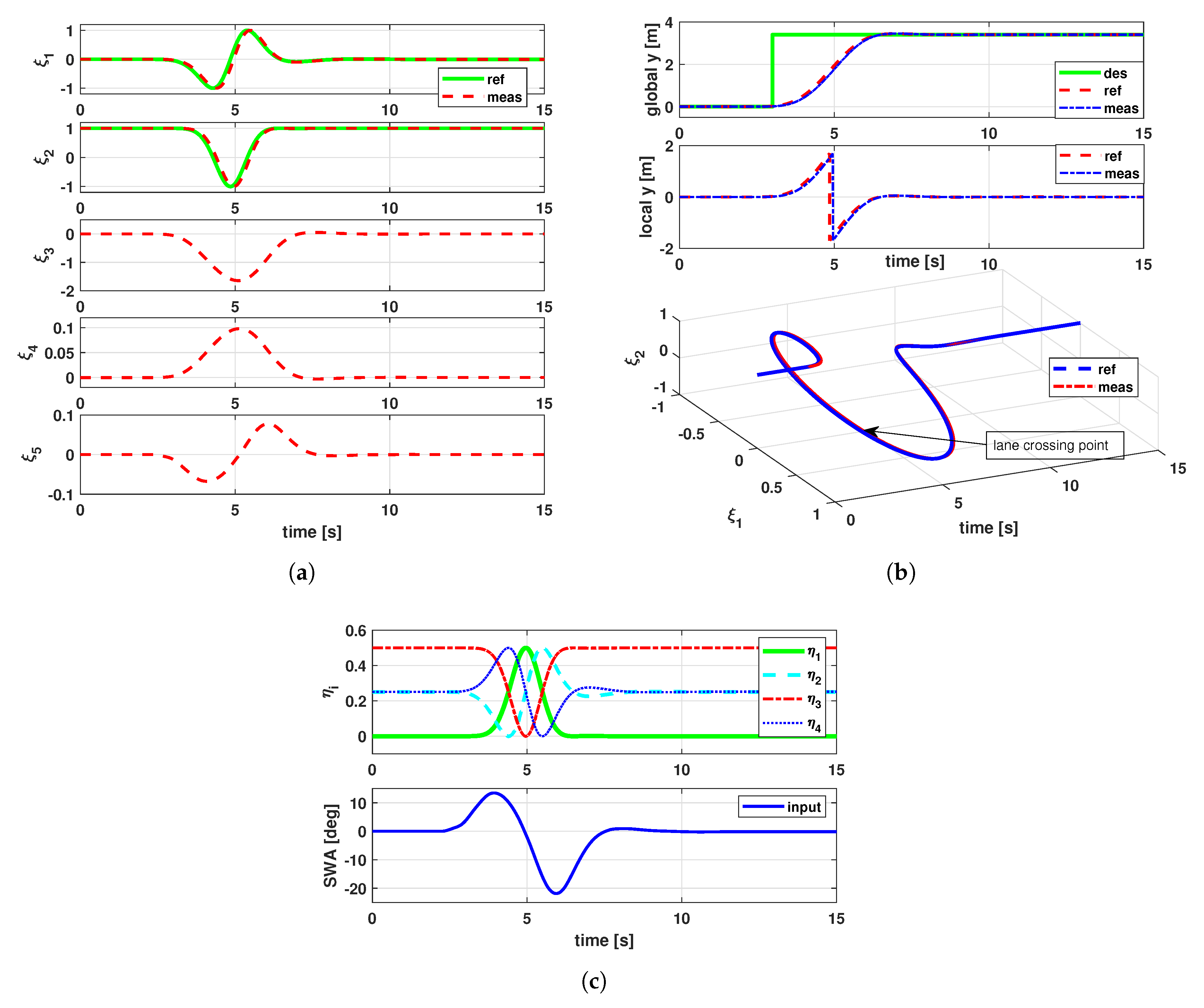
3.2. Scenario 2: Human Driver-Based Trajectory

As discussed earlier, the steering angle obtained when a human driver changes lanes does not follow the sine and cosine trend perfectly. Therefore, in scenario 2, we performed a simulation to determine if the proposed controller exhibits reasonable performance even with this nonsinusoidal reference trajectory. In scenario 2, after 3 s the vehicle started changing lanes for about 3 s. To generate a human driver-based reference for the second scenario, we make a several lane changes using the driver model, which is already implemented in the CarSim. During several lane changes using the human driver model, we logged both ${\xi }_1$ and ${\xi }_2$. Further, we used the logged signals ${\xi }_1$ and ${\xi }_2$ as reference inputs for the proposed ALCS.

Figure 6a shows the reference trajectory and measured state in the cylinder domain. As shown in Figure 6a, the given reference trajectories of ${\xi }_1$ and ${\xi }_2$ are similar but not exactly matched to the sine function. However, unlike scenario 1, the derivative of the reference is continuous; thus the control input changes smoothly during lane change, as shown in Figure 6c In addition, the other states in the cylinder domain, (${\xi }_3$, ${\xi }_4$ and ${\xi }_5$), which are affected by the control input, have similar patterns. Furthermore, it can be seen that a constant value is not maintained in each state. We can infer that the change in the yawrate, which affects the ride quality, is smooth and not abrupt when a human driver changes lanes, as shown in Figure 6a. It is observed that when the lane change begins, the slope of the control input value is smaller than the slope of the moment when crossing the lane, as shown in Figure 6c.

To change lanes to the left, the desired lateral position of the vehicle is set to 3.4 m, as shown by the green line in Figure 6b. Furthermore, using the inverse gluing function in (10), the human characteristics-based trajectories ${\xi }_1$ and ${\xi }_2$ are merged with the reference trajectory, as shown by the red dashed line in Figure 5b. It is observed that when the vehicle crosses the boundary between the original and target lanes at about 5 s, the position of the vehicle in the cylinder domain is $\left({\xi }_1,{\xi }_2\right)=(0,-1)$.

The controller uses sub-obtimal gain, which is obtained by interpolation of the optimized gain for each vertex, as shown in Figure 5c; however, the proposed method provides a reasonable performance. In addition to the significant advantages in terms of computation time, the control performance is remarkable despite the simple linear controller. We expect the proposed method to be suitable for low-cost electronic control units, which cannot handle heavy computations. Furthermore, if necessary, advanced lane change controllers can be applied to improve the control performance, such as model predictive control.

4. Conclusions

In this study, a practical approach for the lane change system of autonomous vehicles is proposed; to the best of our knowledge, this is the first work of its kind in literature. Our cylinder domain approach, which glued the edges of the plane road, change the discrete state to continuous state without jumps. In addition, the proposed cylinder domain makes it possible for the autonomous vehicles to change lanes without considering the lane crossing time. In contrast to the method of integrating the lateral jerk of vehicle to generate the lane change path, the simple sine reference makes it possible to change lanes in the proposed method.

Furthermore, we presented the overall lateral motion controller design procedure for the ALCS. In this study, the LPV method is based on the basic LQ controller for the introduction of the controller design procedure in the cylinder domain; further, it provides reasonable lane change performance. We believe that the proposed method is suitable for low-cost electronic control units because it provides significant performance even with simple calculations using linear convex interpolation. Our future goals include developing advanced controllers in the cylinder domain, such as a model predictive controller and sliding mode controller for ALCS, to improve the tracking performance. Autonomous lane change with varying speed in the cylinder domain is also included in future work.