Bayesian Filtering Multi-Baseline Phase Unwrapping Method Based on a Two-Stage Programming Approach

Featured Application

This paper proposed a novel TSPA-based Bayesian filtering multi-baseline phase unwrapping (MBPU) framework. This framework can provide a theoretical basis for future MBPU studies. The proposed framework can provide an effective theoretical basis for high-precision DEM acquisition.

Abstract

Phase unwrapping (PU) has been a key step in the processing of interferometric synthetic aperture radar (InSAR) data, and its processing accuracy will directly affect the reconstruction results of digital elevation models (DEMs). The traditional single-baseline (SB) PU must be calculated under continuity assumptions. However, multi-baseline (MB) PU can get rid of the limitation of continuity assumption, so reasonable results can be obtained in regions with large gradient changes. However, the poor noise robustness of MBPU has always been a key problem. To address this issue, we transplant three Bayesian filtering methods with a two-stage programming approach (TSPA), and propose corresponding MBPU models. First, we propose a gradient-estimation method based on the first step of TSPA, and then the corresponding PU model is determined according to different Bayesian filtering. Finally, the wrapped phase can be obtained by unwrapping, one by one, using an effective quality map based on heapsort. These methods can improve the robustness of the MBPU methods. More significantly, this paper establishes a novel TSPA-based Bayesian filtering MBPU framework for the first time. This is of great significance for broadening the research of MBPU. The proposed methods experiments on simulated and real MB InSAR datasets. From the results, we can see that the TSPA-based Bayesian filtering MBPU framework can significantly improve the robustness of the MBPU method.

1. Introduction

Interferometric synthetic aperture radar (InSAR) has become a valuable and important method for digital elevation models (DEMs) production [1,2,3,4]. Phase unwrapping (PU), as a difficulty in the research of InSAR data processing, has received widespread attention in recent decades [5,6,7]. Traditional single-baseline PU (SBPU) obtains the unwrapped results based on a phase continuity assumption (PCA). As shown in Equation (1), the gradients of adjacent pixels are limited to $\pi$. Therefore, due to the limitation of the PCA, SBPU cannot obtain better results in regions with large gradient changes [8,9]. Compared to SBPU, the multi-baseline (MB) PU method will increase the gradient ambiguity coefficient from $[-1,1]$ to $[-n,n]$, so that the MBPU method can get rid of the PCA limitation [10,11]. Therefore, the method can obtain ideal results, even in areas with terrain exhibiting phase layover and phase undersampling, which has caused MBPU to receive increasing attention in recent years [12,13,14].

$${\widehat{\Delta }}_{\psi }(k,k-1)=\{\begin{array}{cc}\phi (k)-\phi (k-1)& \left|\phi (k)-\phi (k-1) \right|\le \pi \\ \phi (k)-\phi (k-1)-2\pi & \phi (k)-\phi (k-1)>\pi \\ \phi (k)-\phi (k-1)+2\pi & \phi (k)-\phi (k-1)<-\pi \end{array}$$

(1)

where ${\widehat{\Delta }}_{\psi }(k,k-1)$ is the phase gradient between neighboring pixels. In recent years, more and more MBPU methods have been proposed. These can be divided into two categories. One of methods requires parameter phase estimation, which mainly includes maximum likelihood (ML) estimation [15] and maximum a posterior estimation (MAP) [16]. This type of method solves MB interferograms according to the probability density function, and can obtain the final DEM without PU. However, the noise robustness of the ML method is poor, and the method is extremely susceptible to noise. A small amount of noise will cause an obvious “burr” phenomenon in the unwrapped results, and it requires a sufficient number of high-quality interferograms to obtain satisfactory noise robustness. The MAP method is obtained by establishing a Markov random field, based on the ML method. The MAP method can obtain more accurate DEM reconstruction results, but its reconstruction time is longer, and the optimization steps are more complicated. These shortcomings have limited the application of the ML and MAP methods, and improved methods have been proposed [17,18]. For example, Y. Dong [19] proposed an efficient ML estimation approach of MB SAR interferometry for refined topographic mapping in mountainous areas. The Chinese remainder theorem (CRT) is a representative of the second category of MBPU method [20]. The second category of method is different from the first type, in that it does not require parameter phase estimation. The CRT method can accurately obtain the MBPU results in the absence of noise, but noise is inevitable in real data. To solve this issue, a closed-form CRT-based algorithm was proposed [21]. The MBPU problem was transformed into a cluster-analysis problem, which reduced the shortcomings of the MB unwrapping algorithm with poor noise robustness [10,22]. Thompson [13] proposed a recursive MBPU method that analyzes the relationship between the long-baseline and the short-baseline interferograms, and then uses the short-baseline to obtain the PU results of the long-baseline. B. Jin [23] proposed an MB InSAR PU method based on a mixed integer optimization model. H. Yu [12] proposed a groundbreaking MBPU framework that can introduce an SBPU model to an MBPU method, which has important implications for MBPU research. Y. Lan [24] proposed a refined two-stage programming-based (TSPA) MB approach using a local plane model. In summary, MBPU can obtain better unwraped results, even in areas with complex terrain, but its robustness and efficiency still need further improvement.

The Kalman filter is a better filtering method based on a Bayesian framework. Kim and Griffiths [25] proposed Kalman filtering to solve the problem of PU for the first time. The Kalman filter PU method has attracted wide attention because of its better noise robustness. Loffeld et al. [26] proposed an extended Kalman filter (EKF) PU method. Juan J. Martinez-Espl [27] introduced a particle filter (PF) to the PU method. W. Liu [28] proposed a cubature Kalman filter (CKF) PU method. The Bayesian filtering PU methods are not only applied in the SBPU method but also in MBPU methods. For example, Kim [25] presented an MBPU method based on 3-D Kalman filtering. X. Xie [29] proposed an extended particle filtering (EPF) MBPU algorithm based on an amended matrix pencil model and quantized path-following strategy. However, these Bayesian filtering MBPU methods start at the shortest baseline and proceed to longer and longer baselines. Strictly speaking, these methods do not completely eliminate the limitation of the PCA. Y. Gao [30] proposed a refined TSPA of PU for MB InSAR data using the unscented Kalman filter (TSPAUKF). This method uses the first step of TSPA for gradient estimation, so that TSPAUKF PU can completely get rid of the limitations of the PCA. In this paper, three MBPU methods base on TSPA with better noise robustness are proposed. This paper transplants EKF, CKF, and an unscented information filter (UIF) to the MBPU domain. More meaningfully, based on these methods, we propose a framework of Bayesian filtering MBPU methods based on TSPA. The framework of the MBPU method proposes a gradient estimation method based on TSPA, and uses median filtering method to slightly filter the estimated phase gradients. Finally, the Bayesian filtering method unwraps the pixels, one by one, using an effective quality map based on heapsort. In this paper, we use several sets of simulated data and real data experimental analysis. The results show that the TSPA-based Bayesian filtering methods have better noise robustness, and the framework provides a basis for the introduction of other Bayesian filtering methods to the MBPU method.

The rest of this paper is organized as follows. In Section 2, the MBPU theory and phase gradient estimation method are provided. In Section 3, several TSPA-based Bayesian filtering methods are introduced. In Section 4, we compare and analyze TSPA and TSPA-based Bayesian filtering methods through experiments. A summary and conclusions are provided in Section 5.

2. MBPU Theory and Phase Gradient Estimation

2.1. Mathematical Foundation of MBPU

InSAR technology reconstructs DEM, based on the geometric relationship of its observation. According to the characteristics of the InSAR receiver, the received interferometric phase is compressed between $\left(-\pi ,\pi \right]$, so the wrapped interferometric phase must be unwrapped. The relationship between the wrapped phase and absolute phase can be expressed as:

$$\phi (k)=\psi (k)-2n(k)\pi$$

(2)

where $\psi (k)$, $\phi (k)$, and $n(k)$ are the absolute phase, wrapped phase, and ambiguity number of the $k$ th pixel, respectively. From Equation (2), when the interferometric phase does not contain noise, the absolute phase $\psi (k)$ can be obtained by finding the ambiguity number $n(k)$. According to the observation geometry, we can obtain the following formula:

$$h(k)=\frac{\lambda ·r(k)·\sin (\theta )}{B·2ƛ\pi }·\psi (k)$$

(3)

where $h(k)$ represents the terrain height, $\lambda$ represents the wavelength, $r(k)$ represents the slant range, $\theta$ represents the incidence angle, $B$ represents the normal baseline, and $ƛ$ is 2 for monostatic mode and 1 for bistatic mode. For the same study area, the terrain heights corresponding to different baseline lengths are the same. In this paper, we take the dual-baseline as an example, the equation of the baseline length is:

$$B_2·({\phi }_1(k)+2n_1(k)\pi )=B_1·({\phi }_2(k)+2n_2(k)\pi )$$

(4)

where $B_i(i=1,2)$ represents the baselines of different lengths ($i$ represents different interferograms), $n_i(k)(i=1,2)$ represents the ambiguity number, and ${\phi }_i(k)$ represents the wrapped interferometric phase. Equation (4) is the basic equation for the MBPU method. We cannot solve for two unknowns through one equation. However, because the ambiguity numbers are integers, some methods can enable us to obtain $n_1(k)$ and $n_2(k)$ using only Equation (4).

2.2. Phase Gradient Estimation

Phase gradient estimation is a key step of PU. Whether we use an SBPU or MBPU method, accurate phase gradient estimation method is necessary to obtain a high-precision wrapped phase. According to Equation (4), we can obtain similar equations of a neighboring pixel $k-1$ of pixel $k$, so we will have:

$$B_2·({\phi }_1(k-1)+2n_1(k-1)\pi )=B_1·({\phi }_2(k-1)+2n_2(k-1)\pi )$$

(5)

According to Equation (5) and Equation (4), we can obtain as follows:

$$B_2·({\phi }_1(k)-{\phi }_1(k-1)+2(n_1(k)-n_1(k-1))\pi )=B_1·({\phi }_2(k)-{\phi }_2(k-1)+2(n_2(k)-n_2(k-1))\pi )$$

(6)

We can further rewrite Equation (6) as:

$$B_2·({\phi }_1(k)-{\phi }_1(k-1)+2(\widehat{\Delta }{n}_1(k,k-1))\pi )=B_1·({\phi }_2(k)-{\phi }_2(k-1)+2(\widehat{\Delta }{n}_2(k,k-1))\pi )$$

(7)

where $\widehat{\Delta }{n}_1(k,k-1)=n_1(k)-n_1(k-1)$ and $\widehat{\Delta }{n}_2(k,k-1)=n_2(k)-n_2(k-1)$. From the Equation, it can be seen that $\widehat{\Delta }{n}_1(k,k-1)$ and $\widehat{\Delta }{n}_2(k,k-1)$ are the gradient information between neighboring pixels, and they are both integers. So, we can obtain them by the CRT-based optimization model:

$$\arg \underset{\begin{array}{l}\widehat{\Delta }{n}_1(k,k-1)\\ \widehat{\Delta }{n}_2(k,k-1)\end{array}}{\min }\left|R(\widehat{\Delta }{n}_1(k,k-1),\widehat{\Delta }{n}_2(k,k-1))\right|, \widehat{\Delta }{n}_1(k,k-1),\widehat{\Delta }{n}_2(k,k-1)\in \mathrm{integer}$$

(8)

where $R(\widehat{\Delta }{n}_1(k,k-1),\widehat{\Delta }{n}_2(k,k-1))=B_2·(({\phi }_1(k)-{\phi }_1(k-1))+2(\widehat{\Delta }{n}_1(k,k-1))\pi )-B_1·(({\phi }_2(k)-{\phi }_2(k-1))+$$2(\widehat{\Delta }{n}_2(k,k-1))\pi )$. According to the above equations, we can obtain the ambiguity numbers of the gradient, which is the first step of TSPA.

We assume that an interferometric phase is $M\times N$ pixels. According to Equation (8), we can obtain the ambiguity numbers of these gradients. The phase gradients can be obtained based on the relationship between a point and its neighbors. Therefore, the estimated gradients can be obtained by the following formula:

$$\{\begin{array}{cc}\overline{{\delta }_{i_V}}& ={\psi }_i(m+1,n)-{\psi }_i(m,n)={\phi }_i(m+1,n)-{\phi }_i(m,n)+2·\pi ·\widehat{\Delta }{n}_{i_V}\\ & =s_{i_V}+2·\pi ·\widehat{\Delta }{n}_{i_V}\\ & ={\overline{s}}_{i_V}+2·\pi ·\overline{\Delta }{n}_{i_V}+{\omega }_{i_V}\\ \overline{{\delta }_{i_H}}& ={\psi }_i(m,n+1)-{\psi }_i(m,n)={\phi }_i(m,n+1)-{\phi }_i(m,n)+2·\pi ·\widehat{\Delta }{n}_{i_H}\\ & =s_{i_H}+2·\pi ·\widehat{\Delta }{n}_{i_H}\\ & ={\overline{s}}_{i_H}+2·\pi ·\overline{\Delta }{n}_{i_H}+{\omega }_{i_H}\end{array}$$

(9)

where $\overline{{\delta }_{i_V}}$ and $\overline{{\delta }_{i_H}}$ represent the gradients after slight median filtering, respectively; $\widehat{\Delta }{n}_{i_V}$ and $\widehat{\Delta }{n}_{i_H}$ represent the gradient ambiguity numbers; ${\overline{s}}_{i_V}$ and ${\overline{s}}_{i_H}$ represent the wrapped phase gradients without noise; $\overline{\Delta }{n}_{i_V}$ and $\overline{\Delta }{n}_{i_H}$ represent the gradient ambiguity numbers without noise; ${\omega }_{i_V}$ and ${\omega }_{i_H}$ represent the gradient estimation errors. As can be seen from Equation (9), the gradients estimation method proposed in this paper is not limited by the PCA.

3. Bayesian Filtering MBPU Method

The Bayesian filtering method has been widely used in various fields. The first step of the Bayesian filtering method is to obtain the corresponding state equation and observation equation, according to the specific problem. Then, the state value and the variance of the state equation are predicted, according to the state equation. Finally, we update the data according to the observation equation. As the Bayesian filtering method involves obtaining the unwrapped phase through the state estimation method, not a simple phase gradient summation method, it has also been widely used in PU. To address the MBPU problem, we can obtain the corresponding state equation and observation equation as follows:

$$\{\begin{array}{cc}{\psi }_i(k)& ={\psi }_i(k-1)+{\delta }_i(k-1)+{\omega }_i(k-1)\\ & =f_i\left[{\psi }_i(k-1)\right]+{\omega }_i(k-1)\\ {\varphi }_i(k)& =\left\{\begin{array}{c}\sin ({\psi }_i(k))\\ \cos ({\psi }_i(k))\end{array}\right\}+\left\{\begin{array}{c}{v}_{i_1}(k)\\ v_{i_2}(k)\end{array}\right\}=h_i\left[{\psi }_i(k)\right]+v_i(k)\end{array}$$

(10)

where ${\psi }_i(k-1)$ represents the true unwrapped; ${\delta }_i(k-1)$ and ${\omega }_i(k-1)$ represent the true phase gradient and its estimation error;$f_i\left[{\psi }_i(k-1)\right]$ represents the evolution model; $h_i[{\psi }_i(k)]$ represents the ideal observation vector; and $v_i(k)$ represents the observation variances. Equation (10) is the state equation and observation equation of the Bayesian filtering MBPU method, upon which we base the Bayesian filtering MBPU framework proposed in this paper. This paper will propose several MBPU models of Bayesian filtering.

3.1. Multi-Baseline EKFPU Algorithm

EKF further applies the Kalman filter theory to the nonlinear field, and it has been widely used in satellite positioning and signal processing. EKF expands the nonlinear function into a Taylor series and omits higher-order terms. Generally applicable to weakly nonlinear systems, the filtering performance is poor in the case of strong nonlinearity. Therefore, TSPAEKF method is more suitable for obtaining unwrapped phase with uniform noise distribution. Based on Equation (10), the proposed TSPAEKF method one-step prediction equation is:

$$\{\begin{array}{l}{\overrightarrow{\psi }}_i^{-}(k)={\psi }_i(k-1)+{\delta }_i(k-1)\\ P_{i_{\psi \psi }}^{-}(k)=P_i(k-1)+Q_i(k-1)\end{array}$$

(11)

where ${\overrightarrow{\psi }}_i^{-}(k)$ represents the predicted value of the unwrapped phase, and $P_{i_{\psi \psi }}^{-}(k)$ represents the prediction error covariance matrix of ${\overrightarrow{\psi }}_i^{-}(k)$. According to the EKF model, we can obtain the unwrapped phase estimate ${\psi }_i(k)$ and its corresponding estimated variance matrix $P_{i_{\psi \psi }}(k)$ by the following formula:

$$\{\begin{array}{l}{H}_i(k)=\frac{\delta }{\delta \psi }{h}_i\left[{\overrightarrow{\psi }}_i^{-}(k)\right]={\left[\cos ({\overrightarrow{\psi }}_i^{-}(k)),-\sin ({\overrightarrow{\psi }}_i^{-}(k))\right]}^T\\ {\ell }_i(k)=P_{i_{\psi \psi }}^{-}(k)H_i^T(k)\left(H_i(k)·P_{i_{\psi \psi }}^{-}(k)·H_i^T(k)+R_i(k)\right)\\ {\psi }_i(k)={\overrightarrow{\psi }}_i^{-}(k)+{\ell }_i(k)·{[{\varphi }_i(k)-H_i(k){\varphi }_i^{-}(k)]}^T\\ P_{i_{\psi \psi }}(k)=P_{i_{{}_{\psi \psi }}}^{-}(k)-{\ell }_i(k)·H_i(k)·P_{i_{\psi \psi }}^{-}(k)\end{array}$$

(12)

where $H_i(k)$ is the parameter of the measurement system, and ${\ell }_i(k)$ is the gain matrix. Equations (11) and (12) give TSPAEKF models.

3.2. Multi-Baseline CKFPU Algorithm

The CKF filter uses the spherical-radial criterion to approximate the state posterior mean and covariance, and uses $2n$ cubature points of the same weight to obtain new state points through the system equation. Then, a prediction point of the state at the next moment is obtained. This process does not require the calculation of the complex Jacobian matrix, and it has a good filtering effect. However, the weights of the Cubature points of CKF are equal and appear symmetrically. Therefore, the accuracy of TSPACKF is lower than the other two proposed methods. TSPACKF is more suitable for fast PU with less noise. According to CKF, the cubature points and weights of TSPACKF can be expressed as:

$${\Im }_j(k)=\sqrt{\frac{\Re }{2}}{[1]}_j, b_j=\frac{1}{\Re }$$

(13)

where ${\Im }_j(k)$ is the cubature points, $b_j$ is the weight. In TSPACKF method, $\Re =2$,$[1]=\left[\begin{array}{cc}1& 0\\ 0& 1\end{array}\right]$. We assume that $S_{i_{\psi \psi }}(k)$ is the factoring error covariance, $X_j(k)$ is the cubature point, and $Z_j(k)$ is the jth propagated cubature point. Therefore, we can obtain the equation as:

$$\{\begin{array}{l}{S}_{i_{\psi \psi }}(k)=Chol[P_{i_{\psi \psi }}^{-}(k)]\\ X_j(k)=S_{i_{\psi \psi }}(k)b_j+{\overrightarrow{\psi }}_i^{-}(k)\\ Z_j(k)=h(X_j(k),v_j(k))\end{array}$$

(14)

where $Chol[·]$ is the Cholesky decomposition, and $v_j(k)$ is the observation variance. According to CKF theory, we can obtain the equation as:

$$\{\begin{array}{l}{\varphi }_i^{-}(k)={\displaystyle \sum _{i=1}^m{b}_j{Z}_j(k)}\hfill \\ \begin{array}{l}{P}_{i_{\varphi \varphi }}^{-}(k)={\displaystyle \sum _{j=1}^m{b}_j{Z}_j(k)Z_j^T(k)-{\varphi }_i^{-}(k){({\varphi }_i^{-}(k))}^T+R_i(k)}\\ P_{i_{\psi \varphi }}^{-}(k)={\displaystyle \sum _{j=1}^m{b}_j{X}_j(k)Z_j^T(k)-{\overrightarrow{\psi }}_i^{-}(k){({\overrightarrow{\psi }}_i^{-}(k))}^T}\end{array}\hfill \end{array}$$

(15)

where ${\varphi }_i^{-}(k)$ represents the predicted unwrapped phase; $P_{i_{\varphi \varphi }}^{-}(k)$ represents the prediction error covariance matrix; and $P_{i_{\psi \varphi }}^{-}(k)$ represents the cross-covariance matrix of the predicted measurements. Therefore, we can obtain the unwrapped phase and its corresponding error covariance matrix as the following:

$$\{\begin{array}{l}{\ell }_i(k)=P_{i_{\psi \varphi }}^{-}(k)/P_{i_{\varphi \varphi }}^{-}(k)\hfill \\ {\psi }_i(k)={\overrightarrow{\psi }}_i^{-}(k)+{\ell }_i(k)·{[{\varphi }_i(k)-{\varphi }_i^{-}(k)]}^T\hfill \\ P_{i_{\psi \psi }}(k)=P_{i_{{}_{\psi \psi }}}^{-}(k)-{\ell }_i(k)·P_{i_{\varphi \varphi }}^{-}(k)·{\ell }_i{(k)}^T\hfill \end{array}$$

(16)

Equations (10), (11), and (13)–(16) are the equations of the TSPACKF method.

3.3. Multi-Baseline UIFPU Algorithm

UIF is a newly proposed nonlinear filtering method based on the UKF. UIF improves the robustness of the UKF model by adding the information matrix and its corresponding information state vector to the UKF model. UIF performs deterministic sampling based on UT transformation, and uses a series of specified samples to approximate the posterior probability density of the system state. Therefore, TSPAUIF is more suitable to obtain the phase of complex noise regions. The sigma points can be obtained by the following formula:

$$\{\begin{array}{l}{\xi }_0(k-1)={\overrightarrow{\psi }}_i(k-1)\\ {\xi }_j(k-1)={\overrightarrow{\psi }}_i(k-1)+\left\{\sqrt{(n_{\psi }+\lambda )P_{i_{\psi \psi }}(k-1)}\right\}{ }_j\begin{array}{cc}& j=1,2,\dots ,n_{\psi }\end{array}\\ {\xi }_j(k-1)={\overrightarrow{\psi }}_i(k-1)-\left\{\sqrt{(n_{\psi }+\lambda )P_{i_{\psi \psi }}(k-1)}\right\}{ }_j\begin{array}{cc}& j=n_{\psi }+1,n_{\psi }+2,\dots ,2n_{\psi }\end{array}\end{array}$$

(17)

where $n_{\psi }$ is the dimension of the state variable (i.e., $n_{\psi }=1$); $\lambda ={\omega }^2\left(n_{\psi }+\kappa \right)-n_{\psi }$, $\omega$, $l$, and $\kappa$ are parameters used to adjust the sigma points. In this paper, $\omega =0.01$, $l=2$, and $\kappa =0$. Therefore, we can obtain the one-step prediction equation as:

$$\{\begin{array}{l}{\chi }_j^{-}(k)=f_i\left[{\xi }_j(k-1)\right]\hfill \\ {\overrightarrow{\psi }}_i^{-}(k)={\displaystyle \sum _{i=0}^{2n_{\psi }}{b}_j^m{\chi }_j^{-}(k)}\hfill \\ P_{i_{\psi \psi }}^{-}(k)={\displaystyle \sum _{i=0}^{2n_{\psi }}{b}_j^c\left[{\chi }_j^{-}(k)-{\overrightarrow{\psi }}_i^{-}(k)\right]{\left[{\chi }_j^{-}(k)-{\overrightarrow{\psi }}_i^{-}(k)\right]}^T+Q_i(k-1)}\hfill \end{array}$$

(18)

We let $\wp (k)$ and $\widehat{\wp }(k)$ be the information matrix and its corresponding information state vector, respectively, at pixel $k$. We can obtain $\wp (k)$ and $\widehat{\wp }(k)$ by the following formula:

$$\{\begin{array}{l}\wp (k)=[P_{i_{\psi \psi }}^{-}(k){]}^{-1}\hfill \\ \widehat{\wp }(k)=\wp (k){\overrightarrow{\psi }}_i^{-}(k)\hfill \end{array}$$

(19)

We can obtain ${\varphi }_i^{-}(k)$ and $P_{i_{\varphi \varphi }}^{-}(k)$ using the following formula:

$$\{\begin{array}{l}{\xi }_j^{-}(k)=h_i\left[{\chi }_j^{-}(k)\right]\hfill \\ {\varphi }_i^{-}(k)={\displaystyle \sum _{j=0}^{2n_{\psi }}{b}_j^m{\xi }_j^{-}(k) }\hfill \\ P_{i_{\varphi \varphi }}^{-}(k)={\displaystyle \sum _{j=0}^{2n_{\psi }}{b}_j^c[{\xi }_j^{-}(k)-{\varphi }_i^{-}(k)]}·{[{\xi }_j^{-}(k)-{\varphi }_i^{-}(k)]}^T+R_i(k)\hfill \end{array}$$

(20)

where $b_j^m$ and $b_j^c$ are the weights. $b_0^m=\lambda /(n_{\psi }+\lambda )$, $b_0^c=\lambda /(n_{\psi }+\lambda )+(1-{\omega }^2+l)$ and $b_j^m=b_j^c=1/2(n_{\psi }+\lambda )$ can obtain the weights. In this paper, $j=1,2$. We assume that $\varsigma (k)$ represents the information state contribution and $\aleph (k)$ represents and the corresponding associated information matrix. Thus, we can obtain the following:

$$\{\begin{array}{l}\varsigma (k)=\wp (k)P_{i_{\psi \varphi }}^{-}(k){[R(k)]}^{-1}·\left\{{\varphi }_i(k)-{\varphi }_i^{-}(k)+{[P_{i_{\psi \varphi }}^{-}(k)]}^T{[\wp (k)]}^T{\psi }_i^{-}(k)\right\}\\ \aleph (k)=\wp (k)P_{i_{\psi \varphi }}^{-}(k){[R(k)]}^{-1}·{[P_{i_{\psi \varphi }}^{-}(k)]}^T{[\wp (k)]}^T\end{array}$$

(21)

Through the above analysis, we can obtain ${\psi }_i(k)$ and $P_{i_{\psi \psi }}(k)$ as follows:

$$\{\begin{array}{l}\partial (k)=\widehat{\wp }(k)+\varsigma (k)\\ \overline{\wp }(k)=\wp (k)+\aleph (k)\\ P_{i_{\psi \psi }}(k)={[\overline{\wp }(k)]}^{-1}\\ {\psi }_i(k)=\partial (k)/\overline{\wp }(k)\end{array}$$

(22)

The above three models are MBPU methods, based on the Bayesian filtering method proposed in this paper. All three methods can simultaneously perform PU and filtering. For the convenience of expression, the above equations are all expressed in a one-dimensional shape. We can replace $k$ in the formula with $(m,n)$ to represent the two-dimensional method.

We can use Figure 1 to represent the two-dimensional Bayesian filtering PU method. In the figure, the red dots represent the pixel to be unwrapped. First, we find the eight pixels adjacent to the pixel to be unwrapped and find the unwrapped phase. The green rectangle in Figure 1 represents the unwrapped pixels. Then, we obtain the error map according to the coherence coefficient, and obtain the weight values according to the error of the corresponding pixels. Finally, we weight the red dots pixel with green rectangular pixels to obtain the final unwrapped pixels. The red rectangle in Figure 1 represents the final unwrapped pixels.

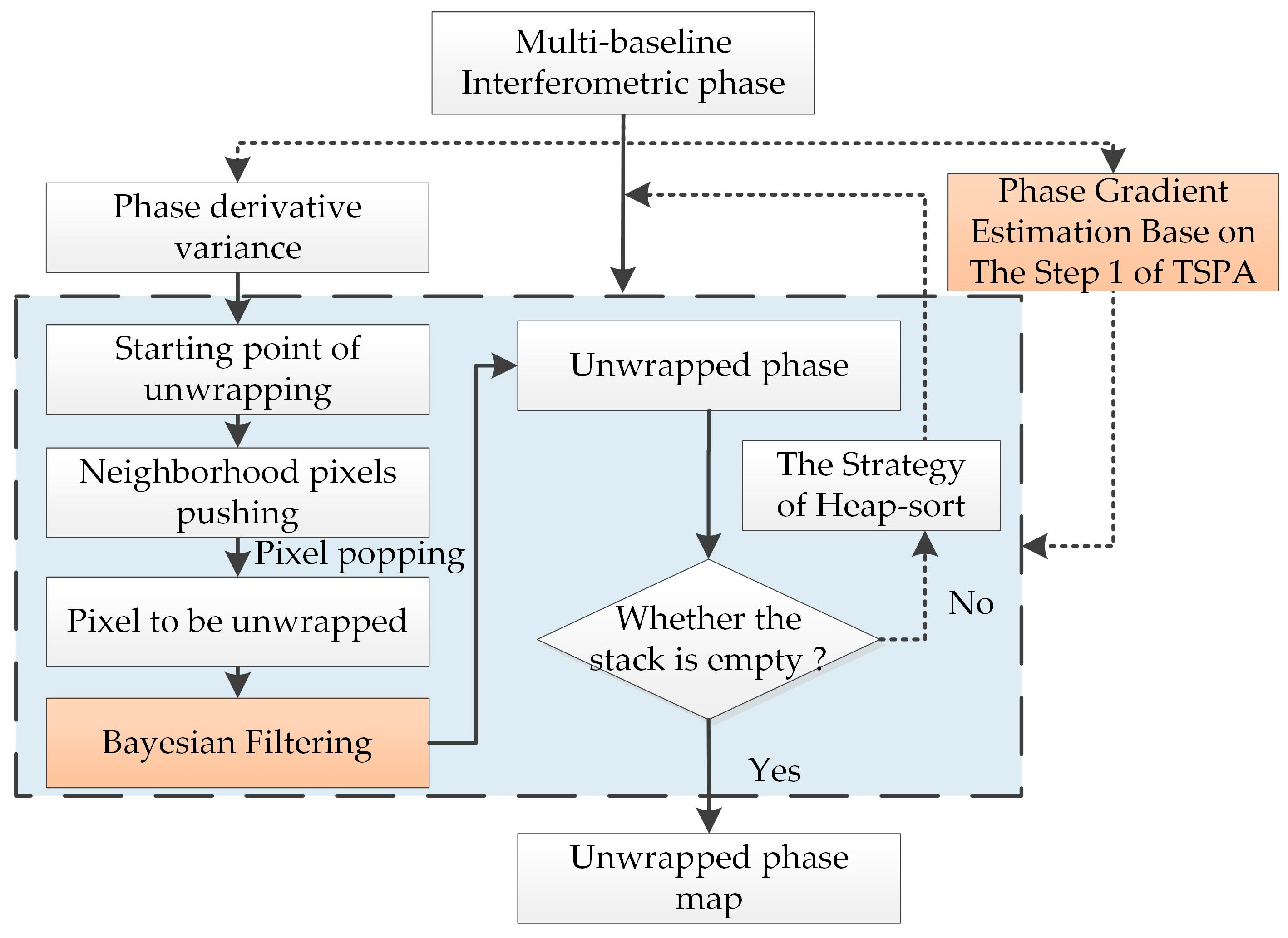
3.4. Framework of TSPA-Based Bayesian Filtering MBPU

In summary, this paper proposes the TSPAEKF, TSPACKF, and TSPAUIF MBPU methods, which are all Bayesian filtering MBPU methods. The MBPU methods with filtering functions proposed in this paper are essentially different from methods proposed in previous research. This paper proposes MBPU methods with good noise robustness, and it is more meaningful that this paper proposes a TSPA-based Bayesian filtering MBPU method framework, whose schematic representation is shown as Figure 2. First, we propose a method based on the first step of TSPA to estimate the distance and azimuth gradients (Equation (9)). The gradients estimated by this method can eliminate the continuity assumption. Then, the equations are obtained that correspond to different Bayesian filtering models. Finally, the unwrapped phase is obtained by unwrapping one pixel at a time according to the heapsort strategy. Through this framework, some other Bayesian filtering methods can also be transplanted to MBPU methods, such as particle filtering, unscented particle filtering, and adaptive filtering. The proposed framework has great significance for broadening the research of MBPU methods.

4. Results and Discussion

In this section, we use two simulated InSAR datasets and a realistic dataset to verify the performance of the proposed TSPA-based Bayesian filtering MBPU methods. The second group of simulation data is used to analyze the noise robustness of different methods. To quantitatively evaluate the performance, the root mean-square error (RMSE) is used to evaluate the results (as Equation (23)):

$$RMSE=\sqrt{E\left[{\Vert \psi -{\psi }_{ture}\Vert }^2\right]}$$

(23)

where $\psi$ is the unwrapped phase collected from the different MBPU methods, ${\psi }_{ture}$ is the reference unwrapped phase, and ${\Vert ·\Vert }^2$ is the quadratic norm. The high-precision ICESat data points are used to verify the accuracy of the realistic dataset.

4.1. Experiment 1

In the first experiment, the performance of the TSPAEKF, TSPACKF, and TSPAUIF methods is verified with a simulated InSAR dataset, and compared with traditional TSPA. Figure 3a is the reference elevation used in this experiment. We can see that the simulated data has complicated terrain fluctuations. Figure 3b shows the reference unwrapped phases with a baseline length of 389.20 m, whereas Figure 3c shows the reference unwrapped phases with a baseline length of 112.10 m. Figure 3d shows the simulated wrapped phases of Figure 3b, and Figure 3e shows the simulated wrapped phases of Figure 3c. From

Table 1. The parameters of simulated interferometric synthetic aperture radar (InSAR) data.

Orbit Altitude	Incidence Angle	Wavelength
600 km	30°	0.24 m
Interferogram	Figure 3d	Figure 3e
Normal Baseline	389.20 m	112.10 m
Mean Correlation Coefficient	0.95	0.95

, we can see the parameters of simulated InSAR data. Figure 3f is the PU result of Figure 3d by TSPA, while Figure 3g–i illustrate the unwrapped phase of Figure 3d obtained by the TSPAEKF, TSPACKF, and TSPAUIF methods, respectively. Figure 3j–m illustrates the errors between Figure 3f–i and Figure 3b. It can be seen from the figure that TSPA produces a significant error transmission phenomenon, due to the influence of noise. Although TSPAEKF, TSPACKF, and TSPAUIF also produce error transmission phenomena, their error transmission areas are significantly smaller than that of TSPA. We can see that different methods produce errors in areas with large gradient changes. This is due to the low interference phase quality in areas with large gradient changes. Although they limit the range of error transmission to a small range, they produce obvious over-smoothing in areas with large gradient changes. Figure 3n is the PU result of Figure 3d by TSPA, while Figure 3o–q illustrates the unwrapped phase of Figure 3b obtained by the TSPAEKF, TSPACKF, and TSPAUIF methods, respectively. Figure 3r–u illustrates the errors between Figure 3n–p and Figure 3c. From the results of the short baseline, it can be seen that these interferograms can obtain better PU results than long baseline interferograms, but that there is still an error transmission phenomenon in the areas of dense noise. The MBPU method of this Bayesian filtering method has better accuracy. In comparison, several Bayesian filtering MBPU methods can obtain more accurate results. From

Table 2. The results of different PU methods in Figure 3j–m,r–u (unit: radians).

PU Method	Long Baseline		Short Baseline
	Figure	RMSE	Figure	RMSE
TSPA	Figure 3j	3.2803	Figure 3r	0.5734
TSPAEKF	Figure 3k	1.6736	Figure 3s	0.4576
TSPACKF	Figure 3l	1.6856	Figure 3t	0.4489
TSPAUIF	Figure 3m	1.6530	Figure 3u	0.4442

, we can see that the long baseline results obtained by TSPA are 3.2803 radians, while the results of TSPAEKF, TSPACKF, and TSPAUIF are 1.6736 radians, 1.6856 radians, and 1.6530 radians, respectively. The short baseline results are similar to the long baseline results. However, the short baseline interferogram is less difficult to unwrap, so the accuracy of these PU methods is very close. Nevertheless, the accuracy of the proposed MBPU methods is still better than that of traditional TSPA. It can be seen from the results that the TSPA-based Bayesian filtering MBPU methods proposed in this paper have a better noise robustness than TSPA. In this experiment, the TSPA consumes 40.55 s, while the TSPAEKF, TSPACKF, and TSPAUIF consume 13.84 s, 11.67 s, and 8.38 s, respectively. The efficiency of proposed TSPA-based Bayesian filtering MBPU methods are better than TSPA.

4.2. Experiment 2

In this experiment, the performance of TSPA and TSPA-based Bayesian filtering MBPU methods was verified using the simulation data in Figure 4d,e. Figure 4a is the employed digital elevation model in the experiment. The data are obtained by MATLAB simulation. Figure 4b,c show the reference unwrapped phases with different normal baseline lengths. Figure 4d shows the simulated wrapped phases of Figure 4b, with added phase noise using 0.95 mean correlation coefficient, and Figure 4e shows the simulated wrapped phases of Figure 4c, with added phase noise using 0.9 mean correlation coefficient. Figure 4f illustrates the unwrapped phase of Figure 4d obtained by TSPA, while Figure 4g–i illustrates the unwrapped phase of Figure 4d obtained by the TSPA-based Bayesian filtering MBPU methods, respectively. Figure 4j–m illustrates the errors between Figure 4f–i and Figure 4b. From the Figure 4f,j, we can see that the traditional TSPA can obtain the PU results. However, due to the influence of noise, an obvious PU error has been generated in the upper right corner. From Figure 4g–I,k–m, it can be seen that the proposed TSPA-based Bayesian filtering MBPU methods can obtain better results than traditional TSPA, and obviously have better noise robustness. However, there is still a small amount of over-smoothing in the gradient-change regions. Figure 4n illustrates the unwrapped phase of Figure 4e obtained by TSPA, while Figure 4o–q illustrates the unwrapped phase of Figure 4e obtained by the TSPA-based Bayesian filtering MBPU methods, respectively. Figure 4r–u illustrates the errors between Figure 4n–q and Figure 4c. It can be seen from the results that, although the short baseline interferogram is easier to unwrap, the result of the traditional TSPA is still not ideal, due to the influence of noise. However, the TSPA-based Bayesian filtering MBPU methods not only obtain great PU results, but have better noise robustness. As can be seen from

Table 3. The results of different PU methods in Figure 4j–m,r–u (unit: radians).

PU Method	Long Baseline		Short Baseline
	Figure	RMSE	Figure	RMSE
TSPA	Figure 4j	2.5464	Figure 4r	1.7760
TSPAEKF	Figure 4k	0.2865	Figure 4s	0.2354
TSPACKF	Figure 4l	0.3731	Figure 4t	0.2795
TSPAUIF	Figure 4m	0.2929	Figure 4u	0.2408

, the long and short baseline PU accuracy of traditional TSPA are 2.5464 radians and 1.7760 radians, respectively. Due to the influence of noise, the accuracy of traditional TSPA is not very good. The TSPA-based Bayesian filtering MBPU methods proposed in this study, especially the TSPAEKF and TSPAUIF methods, can obtain better results. The PU results of TSPACKF are relatively ineffective, but have better noise robustness. The efficiency of proposed TSPA-based Bayesian filtering MBPU methods are 7.97 s, 7.13 s, and 5.28 s, respectively. The efficiency of TSPA is 8.23 s, and it can be seen from the experiment that the proposed methods not only have better robustness, but also have better efficiency.

4.3. Experiment 3

In this experiment, we validate the proposed TSPA-based Bayesian filtering MBPU method with a real MB InSAR datasets. Figure 5a shows the real surface conditions of the study area. From the figure, we can see that the study area contains a large number of high mountains. In

Table 4. The parameters of real multi-baseline (MB) InSAR datasets.

Orbit Altitude	Incidence Angle	Wavelength
514.8 km	36.60°	0.0320 m
Interferogram	Figure 5b	Figure 5c
Normal Baseline	−370.46 m	−127.79 m
Image Size	3040 × 2315 pixels	3040 × 2315 pixels

, we can see the major parameters of the real dataset. Figure 5b is an interferogram with a baseline length of −370.46 m, and Figure 5c is an interferogram with a baseline length of −127.79 m. From Figure 5b,c, the white lines are composed of the ICESat points. The accuracy of these ICESat points is about 14cm. It can be seen from Figure 5a that the research area has obvious mountain undulations, and it was proved [30] that the SBPU method cannot obtain high-precision PU results. Figure 5d–g illustrates the unwrapped phase of Figure 5b obtained by TSPA, and the proposed TSPA-based Bayesian filtering MBPU methods, respectively. Figure 5h–k illustrates the unwrapped phase of Figure 5c obtained by TSPA, and the proposed TSPA-based Bayesian filtering MBPU method, respectively. It can be seen at a glance that the results obtained by different MBPU methods are very similar. This is because the experimental data have less noise and a larger study area. To further compare the performance of different MBPU methods, we provide the DEMs generated from the data of different MBPU results, and use ICESat data points to verify the accuracy of the results of different methods. As can be seen from

Table 5. Root mean-square error (RMSEs) of TanDEM-X DEM assessed using ICESat data points (unit: meters).

PU Method	Long Baseline	Short Baseline
	RMSE	RMSE
TSPA	3.73	3.25
TSPAEKF	3.08	3.04
TSPACKF	3.10	3.10
TSPAUIF	3.05	3.04

, the standard deviations obtained by traditional TSPA method are 3.25 m for Figure 5d and 3.73 m for Figure 5h. The results of TSPAEKF are better than the TSPA method. The standard deviations of the obtained results are 3.08 m for Figure 5e and 3.04 m for Figure 5f. Similar to the previous simulation data results, TSPACKF also has better noise robustness. However, the accuracy of the results is the worst of the three proposed TSPA-based Bayesian filtering MBPU methods. The standard deviations obtained are 3.10 m for Figure 5f and 3.10 m for Figure 5i. TSPAUIF is an improved algorithm, based on TSPAUKF. This method can obtain better results than other methods. Its standard deviations are 3.05 m for Figure 5g and 3.04 m for Figure 5k. Moreover, the efficiency of TSPAEKF, TSPACKF, and TSPAUIF in this experiment are 1133.63 s, 1065.35 s, and 750.37 s, respectively. They are much faster than the efficiency of the TSPA, which required 26,156.58 s. It can be seen from the experimental results that the TSPA-based Bayesian filtering MBPU methods proposed in this paper can obtain better results than traditional TSPA methods, and their efficiency is better.

4.4. Experiment 4

To verify the noise robustness of the proposed TSPA-based Bayesian filtering MBPU methods, this study uses Figure 4b,c as a reference unwrapped phase, to add phase noise with different mean correlation coefficients to the data, and we obtained the wrapped phases. As shown in Figure 6, we added phase noise to the simulated data with phase correlation coefficients of 1, 0.99, 0.98, 0.96, 0.95, 0.93, 0.90, 0.88, 0.85, 0.88, 0.75, and 0.7. It can be seen from the results that when the wrapped phases are without noise, different MBPU methods can accurately obtain the PU results. However, with the decrease of the phase correlation coefficient, the results of traditional TSPA become significantly worse, especially when the correlation coefficient is less than 0.90, as the unwrap phase produces a serious unwrap error phenomenon. However, the proposed TSPA-based Bayesian filtering MBPU methods can still obtain results when the phase correlation coefficients are 0.8, which further validates that the methods are better than the traditional TSPA. However, there are also differences among the TSPA-based Bayesian filtering MBPU methods. For example, when the phase correlation coefficient is 0.93, the long baseline result of TSPACKF produces a phenomenon of unwrap error in the same areas, but this does not occur in the other two methods. This may be caused by different methods of variance estimation. This provides a research point for the more accurate TSPA-based Bayesian filtering MBPU methods proposed in the future.

5. Conclusions

Three TSPA-based Bayesian filtering MBPU methods have been proposed. These proposed methods transplant the EKF, CKF, and UIF to the MBPU methods, respectively. More meaningfully, this paper proposed a TSPA-based Bayesian filtering MBPU framework. We proposed a gradient estimation method based on the first step of TSPA, which can eliminate the limitation of phase gradients by the PCA. Then, the corresponding PU model is determined according to different Bayesian filtering methods. Finally, the TSPA-based Bayesian filtering MBPU method unwraps the pixels, one by one, using an effective quality map based on heapsort. This proposed MBPU framework provides a basis for the research of MBPU methods with filtering functions.

From the results of the simulated data, the TSPA-based Bayesian filtering MBPU methods not only ignore the PCA, but also have good noise robustness. It is further seen through the robustness analysis experiments that TSPA is easily affected by noise. However, TSPA-based Bayesian filtering MBPU methods have great noise robustness. Experiments with a set of TanDEM-X data with topography exhibit severe undulations. In addition, ICESat data points are used to evaluate the accuracy of the DEMs generated by the different methods. The results of the experiments demonstrate that the proposed TSPA-based Bayesian filtering MBPU methods can obtain better results, and are more efficient than the traditional TSPA.

References

1. Ferraiuolo, G.; Federica, M.; Pascazio, V.; Schirinzi, G. DEM Reconstruction Accuracy in Multichannel SAR Interferometry. IEEE Trans. Geosci. Remote Sens. 2009, 47, 191–201. [Google Scholar] [CrossRef]
2. Ghiglia, D.C.; Wahl, D.E. Interferometric Synthetic Aperture Radar Terrain Elevation Mapping from Multiple Observations. In Proceedings of the IEEE 6th Digital Signal Processing Workshop, Albuquerque, NM, USA, 2–5 October 1994; pp. 33–36. [Google Scholar] [CrossRef] [Green Version]
3. Baselice, F.; Ferraioli, G.; Pascazio, V.; Schirinzi, G. Contextual information-based multichannel synthetic aperture radar interferometry: Addressing DEM reconstruction using contextual information. IEEE Signal Process. Mag. 2014, 31, 59–68. [Google Scholar] [CrossRef]
4. Gao, Y.; Zhang, S.; Li, T.; Guo, L.; Chen, Q.; Li, S. A novel two-step noise reduction approach for interferometric phase images. Opt. Lasers Eng. 2019, 121, 1–10. [Google Scholar] [CrossRef]
5. Yu, H.; Lan, Y.; Yuan, Z.; Xu, J.; Lee, H. A Review on Phase Unwrapping in In SAR Signal Processing. IEEE Geosci. Remote Sens. Mag. 2019, 15, 1887–1891. [Google Scholar] [CrossRef]
6. Yu, H.; Lan, Y.; Xu, J.; An, D.; Lee, H. Large-Scale L0-Norm and L1-Norm 2-D Phase Unwrapping. IEEE Trans. Geosci. Remote Sens. 2017, 55, 4712–4728. [Google Scholar] [CrossRef]
7. Yu, H.; Li, Z.; Bao, Z. Residues Cluster-Based Segmentation and Outlier-Detection Method for Large-Scale Phase Unwrapping. IEEE Trans. Image Process. 2011, 20, 2865–2875. [Google Scholar] [CrossRef]
8. Xu, J.; An, D.; Huang, X.; Wang, G. Phase Unwrapping for Large-Scale P-Band UWB SAR Interferometry. IEEE Geosci. Remote Sens. Lett. 2015, 12, 2120–2124. [Google Scholar] [CrossRef]
9. Yu, H.; Lan, Y.; Lee, H.; Cao, N. 2-D phase unwrapping using minimum infinity-norm. IEEE Geosci. Remote Sens. Lett. 2018, 7, 40–58. [Google Scholar] [CrossRef]
10. Yu, H.; Li, Z.; Bao, Z. A Cluster-Analysis-Based Efficient Multibaseline Phase-Unwrapping Algorithm. IEEE Trans. Geosci. Remote Sens. 2011, 49, 478–487. [Google Scholar] [CrossRef]
11. Ferretti, A.; Prati, C.; Rocca, F.; Guarnieri, A.M. Multibaseline SAR interferometry for automatic DEM reconstruction (DEM). In Proceedings of the 3rd ERS Symposium on Space at the Service of Our Environment, Florence, Italy, 17–21 March 1997; pp. 1809–1820. [Google Scholar]
12. Yu, H.; Lan, Y. Robust Two-Dimensional Phase Unwrapping for Multibaseline SAR Interferograms A Two-Stage Programming Approach. IEEE Trans. Geosci. Remote Sens. 2016, 54, 5217–5225. [Google Scholar] [CrossRef]
13. Thompson, D.G.; Robertson, A.E.; Arnold, D.V.; Long, D.G. Multi-baseline interferometric SAR for iterative height estimation. In Proceedings of the IEEE 1999 International Geoscience and Remote Sensing Symposium, Hamburg, Germany, 28 June–2 July 1999; pp. 251–253. [Google Scholar] [CrossRef]
14. Xu, W.; Chang, E.; Kwoh, L.; Lim, H.; Cheng, W. Phase-unwrappingof SAR interferogram with multi-frequency or multi-baseline. In Proceedings of the IGARSS ’94—1994 IEEE International Geoscience and Remote Sensing Symposium, Pasadena, CA, USA, 8–12 August 1994; pp. 730–732. [Google Scholar] [CrossRef]
15. Fornaro, G.; Monti Guarnieri, A.; Pauciullo, A.; De-Zan, F. Maximum likelihood multi-baseline SAR interferometry. IET Radar Sonar Navig. 2006, 153, 279. [Google Scholar] [CrossRef] [Green Version]
16. Ferraiuolo, G.; Pascazio, V.; Schirinzi, G. Maximum a posteriori estimation of height profiles in InSAR imaging. IEEE Geosci.Remote Sens. Lett. 2004, 1, 66–70. [Google Scholar] [CrossRef]
17. Hong, F.; Tang, J.; Lu, P. Multichannel DEM reconstruction method based on Markov random fields for bistatic SAR. Sci. China Inform. Sci. 2015, 58, 1–14. [Google Scholar] [CrossRef] [Green Version]
18. Chirico, D.; Schirinzi, G. Multichannel interferometric SAR phase unwrapping using extended Kalman Smoother. Int. J. Microw. Wirel. Tech. 2013, 5, 429–436. [Google Scholar] [CrossRef]
19. Dong, Y.; Jiang, H.; Zhang, L.; Liao, M. An Efficient Maximum Likelihood Estimation Approach of Multi-Baseline SAR Interferometry for Refined Topographic Mapping in Mountainous Areas. Remote Sens. 2018, 10, 454. [Google Scholar] [CrossRef]
20. Li, X.; Xia, X. A Fast Robust Chinese Remainder Theorem Based Phase Unwrapping Algorithm. IEEE Signal Process. Lett. 2008, 15, 665–668. [Google Scholar] [CrossRef]
21. Yuan, Z.; Deng, Y.; Li, F.; Wang, R.; Liu, G.; Han, X. Multichannel InSAR DEM reconstruction through improved closed-form robust Chinese remainder theorem. IEEE Geosci. Remote Sens. Lett. 2013, 10, 1314–1318. [Google Scholar] [CrossRef]
22. Liu, H.; Xing, M.; Bao, Z. A Cluster-Analysis-Based Noise-Robust Phase-Unwrapping Algorithm for Multibaseline Interferograms. IEEE Trans. Geosci. Remote Sens. 2015, 53, 494–504. [Google Scholar] [CrossRef]
23. Jin, B.; Guo, J.; Wei, P.; Su, B.; He, D. Multi-baseline InSAR phase unwrapping method based on mixed-integer optimisation model. IET Radar Sonar Navig. 2018, 12, 694–701. [Google Scholar] [CrossRef]
24. Lan, Y.; Yu, H.; Xing, M. Refined Two-Stage Programming-Based Multi-Baseline Phase Unwrapping Approach Using Local Plane Model. Remote Sens. 2019, 11, 491. [Google Scholar] [CrossRef] [Green Version]
25. Kim, M.G.; Griffiths, H.D. Phase unwrapping of multibaseline interferometry using Kalman filtering. In Proceedings of the 7th International Conference on Image Processing and its Applications, London, UK, 13–15 July 1999; pp. 251–253. [Google Scholar] [CrossRef]
26. Nies, H.; Loffeld, O.; Wang, R. Phase unwrapping using 2D-Kalman filter—Potential and limitations. In Proceedings of the IEEE International Geoscience and Remote Sensing Symposium, Boston, MA, USA, 7–11 July 2008; pp. 1213–1216. [Google Scholar] [CrossRef]
27. Martinez-Espla, J.J.; Martinez-Marin, T.; Lopez-Sanchez, J.M. An Optimized Algorithm for InSAR Phase Unwrapping Based on Particle Filtering, Matrix Pencil, and Region-Growing Techniques. IEEE Geosci. Remote Sens. Lett. 2009, 6, 835–839. [Google Scholar] [CrossRef]
28. Liu, W.; Bian, Z.; Liu, Z.; Zhang, Q. Evaluation of a Cubature Kalman Filtering-Based Phase Unwrapping Method for Differential Interferograms with High Noise in Coal Mining Areas. Sensors 2015, 15, 16336–16357. [Google Scholar] [CrossRef] [PubMed] [Green Version]
29. Xie, X.; Zeng, Q. Multi-baseline extended particle filtering phase unwrapping algorithm based on amended matrix pencil model and quantized path-following strategy. J. Syst. Eng. Electron. 2019, 30, 78–84. [Google Scholar] [CrossRef]
30. Gao, Y.; Zhang, S.; Li, T.; Chen, Q.; Zhang, X.; Li, S. Refined Two-Stage Programming Approach of Phase Unwrapping for Multi-Baseline SAR Interferograms Using the Unscented Kalman Filter. Remote Sens. 2019, 11, 199. [Google Scholar] [CrossRef] [Green Version]
Figure 1. Simple flowchart of two-dimensional Bayesian filtering phase unwrapping (PU) method.
Applsci 10 03139 g001
Figure 2. Schematic representation of two-stage programming approach (TSPA)-based Bayesian filtering multi-baseline phase unwrapping (MBPU) method framework.
Applsci 10 03139 g002
Figure 3. (a) Digital elevation model (DEM) for simulation data (unit: m). (b,c) Reference unwrapped phases ((b) long and (c) short baseline length). (d,e) Simulated wrapped phases of (b,c). (fi) PU results of (b) obtained by (f) TSPA, (g) extended Kalman filter (TSPAEKF), (h) cubature Kalman filter (TSPACKF), and (i) unscented information filter (TSPAUIF). (jm) Errors between (b) and PU results (fi). (nq) PU results of (c) obtained by (n) TSPA, (o) TSPAEKF, (p) TSPACKF, and (q) TSPAUIF. (ru) Errors between (c) and PU results (nq).
Applsci 10 03139 g003
Figure 4. (a) Digital elevation model (DEM) for simulation data. (b,c) Reference unwrapped phases ((b) long and (c) short baseline length). (d,e) Simulated wrapped phases of (b,c). (fi) PU results of (b) obtained by (f) TSPA, (g) TSPAEKF, (h) TSPACKF, and (i) TSPAUIF. (jm) Errors between (b) and PU results (fi). (nq) PU results of (c) obtained by (n) TSPA, (o) TSPAEKF, (p) TSPACKF, and (q) TSPAUIF. (ru) Errors between (c) and PU results (nq).
Applsci 10 03139 g004aApplsci 10 03139 g004b
Figure 5. (a) Google Earth image of the study area. (b,c) Real interferograms with (b) long, and (c) short baseline lengths. (dg) PU results of (b) obtained by (d) TSPA, (e) TSPAEKF, (f) TSPACKF, and (g) TSPAUIF. (hk) PU results of (c) obtained by (h) TSPA, (i) TSPAEKF, (j) TSPACKF, and (k) TSPAUIF.
Applsci 10 03139 g005
Figure 6. Robustness analysis using simulated data of Figure 4b,c with different methods.
Applsci 10 03139 g006