Parametrized Analysis and Multi-Objective Optimization of Supercritical CO₂ (S-CO₂) Power Cycles Coupled with Parabolic Trough Collectors

Abstract

Supercritical CO₂ (S-CO₂) Brayton cycles have become an effective way in utilizing solar energy, considering their advantages. The presented research discusses a parametrized analysis and systematic comparison of three S-CO₂ power cycles coupled with parabolic trough collectors. The effects of turbine inlet temperature and pressure, compressor inlet temperature, and pressure on specific work, overall efficiency, and cost of core equipment of different S-CO₂ Brayton cycles are discussed. Then, the two performance criteria, including specific work and cost of core equipment, are compared, simultaneously, between different S-CO₂ cycle layouts after gaining the Pareto sets from multi-objective optimizations using genetic algorithm. The results suggest that the simple recuperation cycle layout shows more excellent performance than the intercooling cycle layout and the recompression cycle layout in terms of cost, while the advantage in specific work of the intercooling cycle layout and the recompression cycle layout is not obvious. This study can be useful in selecting cycle layout using solar energy by the parabolic trough solar collector when there are requirements for the specific work and the cost of core equipment. Moreover, high turbine inlet temperature is recommended for the S-CO₂ Brayton cycle using solar energy.

1. Introduction

Solar energy has played an important role in sustainability. The main routes to harvest solar energy are by concentrating solar thermal power (CSP) and solar photovoltaics (PV) [1]. There is a lot of research on PV, including economics and environmental performance [2,3]. Compared with the PV generation, CSP has certain advantages in the power generation scale. At present, multiple kinds of CSP technology, including the parabolic trough collector (PTC) [4], the linear Fresnel reflector [5], and the solar power tower (SPT) [6] have been reported. Among them, parabolic trough (PT) can be considered the most mature technology for CSP plants due to projects conducted by the United States [7] and Spain [8].

At present, the Rankine cycle is the most common power generation cycle in CSP technology, which uses parabolic trough collectors, while organic working fluids and water are commonly adopted. However, these forms of power generation face barriers, including the use of working fluids that are easy to aggravate global warming, and high investment costs [9]. The performance of the Organic Rankine Cycle (ORC) is limited by chemical degradation and auto-ignition at high temperatures [10]. Thus, ORC is a better power cycle choice only when the temperature of the heat source is lower than 300 °C, according to the research data of some literatures [11]. In addition, the thermal characteristics of steam lead to the use of multi-stage turbines and complex power plants, which will undoubtedly increase the costs.

Supercritical carbon dioxide (S-CO₂) has been identified as an attractive working fluid with lots of advantages [12]. Firstly, CO₂ is inexpensive, non-toxic, nontoxic, inert, abundant, and easy to reach critical point (7.38 MPa, 304.25 K) [13]. The low compressibility, viscosity, and the high density of S-CO₂ can be helpful to achieve high efficiency and compact mechanical structures in the power cycles [14,15]. Finally, compared with the Rankine cycle, it can save when it comes to the cost of several valves and condensers, because of the little phase change in the S-CO₂ power cycle. Hence, more attention has been paid to the application of the S-CO₂ Brayton cycle, especially in the fields of waste-heat recovery [12], nuclear power generation [16], and CSP [17,18].

Nowadays, most research on the application of SCO₂ in CSP technology are SPT, which can take advantage of the higher working temperatures [19]. Binotti et al. [20] discussed the thermodynamic assessment of three S-CO₂ cycles with turbine inlet temperatures up to 800 °C. Recompression with Main Compression Intercooling (RMCI) configuration was considered as the optimal loop structure in the study, which reached electric efficiency of 24.5% under the design condition. Turchi et al. [21] compared the efficiencies of different S-CO₂ Brayton cycle layouts coupled with SPT. The partial-cooling and inter-cooling cycle with reheating could achieve efficiency of 50%. Padilla et al. [22] also carried out the energy and exergy analysis for different S-CO₂ cycle layouts using SPT.

However, SPT is not a mature technology, and the plants using SPT have limitation of large floor space. Therefore, it should be considered to use S-CO₂ cycles with PTC. The above conclusions are made in the case of heat source temperatures above 500 °C (even above 600 °C). However, CSP using conventional PTC at maximum temperatures, in the range between 350 °C and 400 °C, is common technology. Hence, it is still necessary for the comparative study of S-CO₂ cycles coupled with PTC. In fact, some researchers have carried out the research of S-CO₂ cycles coupled with PTC [23,24]. However, their research is based on the performance of the system, and there are few comparative studies on the economy between different types of cycles.

Moreover, multi-objective optimization has been used in many other previous works and proved to be an effective method. Wang et al. [25] put forward a systematic comparison of different S-CO₂ Brayton cycle layouts based on multi-objective optimizations. Their results suggested that the inter-cooling cycle layout and the partial-cooling cycle layout provided the most excellent performances. Padilla et al. [26] also performed multi-objective optimizations of the supercritical CO₂ Brayton cycles integrated with a solar receiver. However, these studies did not consider economic comparisons between the power cycles. In fact, economic cost is also considered as one of the important indicators of comparisons between different cycles [27].

Based on the above literature review, we introduce the preliminary economic analysis of the comparison of the S-CO₂ cycles with PTC. The primary contributions of this work are as follows:

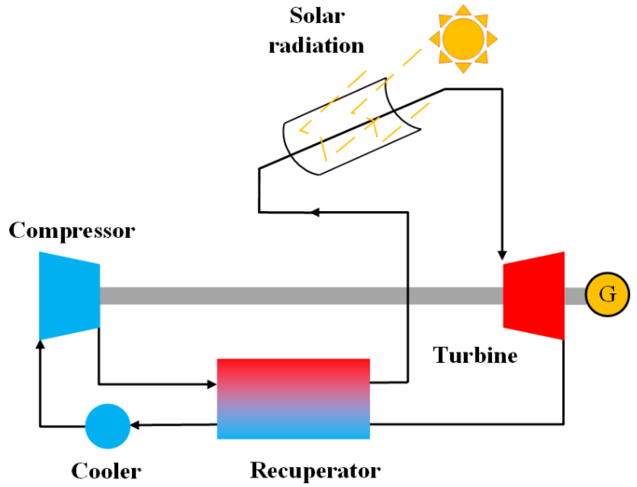
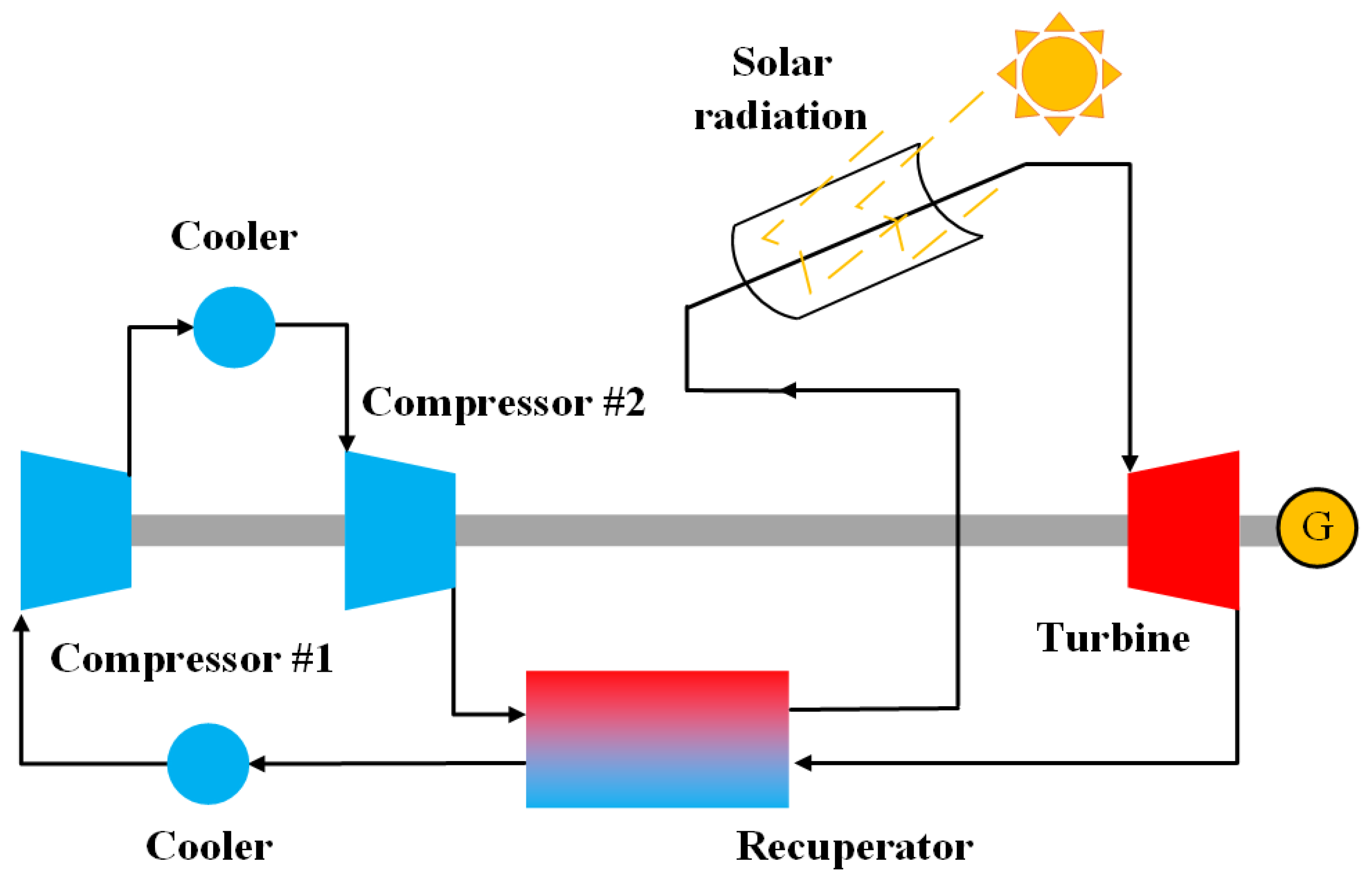
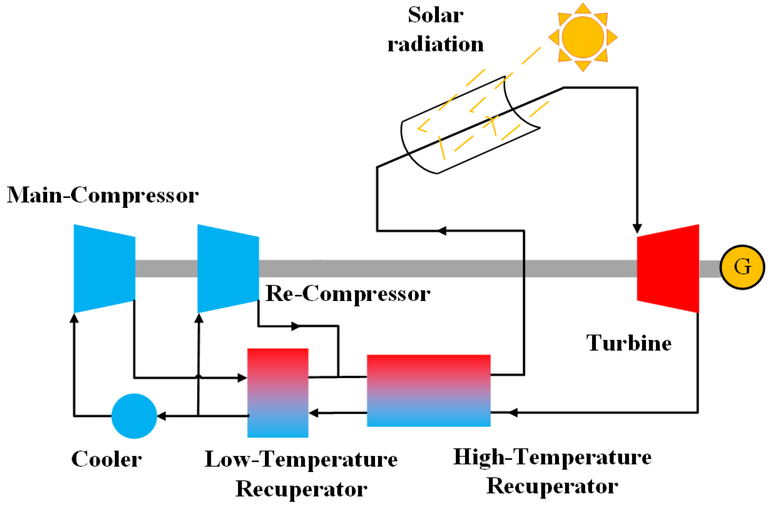
• Three S-CO₂ power cycles coupled with PTC (namely, simple regeneration, intercooling and re-compression) are established and their parameters are analyzed for preliminary comparison.
• A multi-objective optimization method using genetic algorithm (GA) is presented to compare the performance, including thermodynamic performance and preliminary economic cost of cycles. The advantages and disadvantages of the three cycle kinds are thoroughly compared.
• The sensitivity analysis of a typical optimization result of a simple regeneration cycle is carried out; the influence of different parameters on system performance is obtained.

This work can provide a solid foundation for the fundamental design and construction of S-CO₂ Brayton cycles. We hope that this research will ignite interest in the application of S-CO₂ cycles coupled with PTC and the performance comparison of cycles considering thermodynamics and economics.

2. Description of the Research Systems

The S-CO₂ Brayton cycle based on solar energy has the same structure as that of a conventional heat source. Core components of the power cycle include the turbine, generator, heat regenerator, cooler, and compressor. The thermal cycles studied in this paper include three types, simple recuperated cycle, intercooling cycle, and the recompression cycle. Solar receivers are adopted to absorb solar radiation heat to warm S-CO₂.

The simple recuperated cycle is shown in Figure 1, which has been presented by Feher [28]. The working fluid S-CO₂ is cooled before compressing to an applicable pressure for the compressor. In the recuperator, cold S-CO₂ absorbs heat from hot S-CO₂ exiting from the turbine outlet. Moreover, before expanding in the turbine, the pre-heated S-CO₂ further absorbs heat from the solar receiver.

Figure 2 shows the layout of the intercooling cycle, which has been previously presented by Ahn et al. [29]. Compared to the simple recuperated cycle, the intercooling cycle adopts another cooler to help reduce the compression work. It can be accomplished since the temperature of the compressed S-CO₂ is further reduced. This arrangement can also generate a larger pressure ratio. Moreover, other components in the intercooling cycle have high similarity with those in the above cycle.

Figure 3 presents the recompression cycle, which has also been adopted by Moisseytsev et al. [30]. This kind of cycle has high similarity with the simple recuperated cycle. Nevertheless, the components are of different numbers and arrangements. Before the cooler, there are two kinds of recuperators, which are used in high-temperature and low-temperature, respectively. After regeneration, S-CO₂ splits into two parts. Part of the fluid flows through the cooler and then enters the main-compressor while the other part flows into the re-compressor. The fluid from the main-compressor outlet flows into the low-temperature recuperator and the high-temperature recuperator. The fluid from the outlet of the re-compressor flows only into the high-temperature recuperator. In addition, other components are similar with the above two configurations.

It should be noticed that due to the inexistence of a thermal energy storage device, the systems would mostly work under off-design conditions. As shown in previous studies, the performance of systems change dramatically [31,32]. Therefore, we can add a thermal energy storage device to the systems to ensure that the systems operate in a steady state. However, the discussion of a thermal energy storage device is not the focus of this paper, so the relevant description is omitted.

3. Modeling of the System

The purpose is to compare the thermodynamic characteristics and preliminary performance of the three different power cycles after respective optimization. The systems are modeled in a steady state with the software MATLAB; the properties of CO₂ are obtained from the software NIST REFPROP. In the meantime, the modeling can be adopted to analyze preliminary performance and realize the optimizations.

The modeling process is based on typical simplified assumptions, which are commonly utilized for a power system evaluation problem. They are listed as follows:

• The cycle is considered steady during calculation.
• The effects of kinetic and gravitational terms are neglected in the calculations.
• The pressure drops and heat loss are neglected.

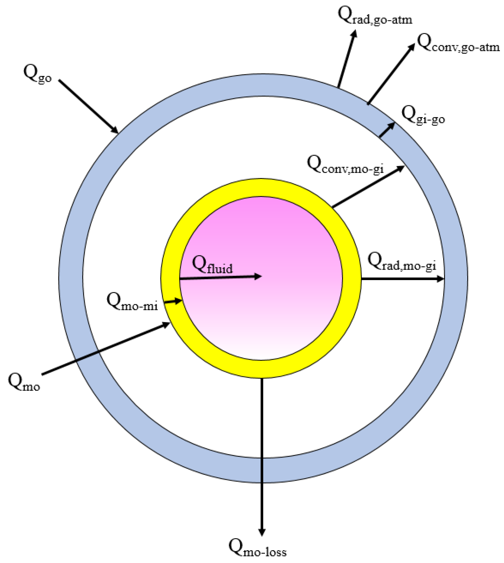
3.1. Solar Collector

Figure 4 shows the energy balance at the cross section of the parabolic trough solar collector used in this study. The outer blue ring represents the glass envelope while the inner yellow ring represents the metal heat-absorbing tube in the figure. The equations of energy can be written as [33]:

$$Q_{\mathrm{fluid}}=Q_{\text{mo-mi}}$$

(1)

$$Q_{\mathrm{mo}}=Q_{\text{mo-mi}}+Q_{\mathrm{conv},\text{mo-gi}}+Q_{\mathrm{rad},\text{mo-gi}}+Q_{\text{mo-loss}}$$

(2)

$$Q_{\mathrm{gi-go}}=Q_{\mathrm{conv},\text{mo-gi}}+Q_{\mathrm{rad},\text{mo-gi}}$$

(3)

$$Q_{\mathrm{conv},\text{go-atm}}+Q_{\mathrm{rad},\text{go-atm}}=Q_{\text{gi-go}}+Q_{\mathrm{go}}$$

(4)

where Q is quantity of heat, subscript fluid indicates the working fluid, subscript mo-mi the transmitting process from the outer surface of the metal absorber to the inner surface, subscript mo indicates the outer surface of absorber. Subscript conv,mo-gi indicates the convection heat transfer process from absorber to the inner surface of glass envelope, subscript rad,mo-gi indicates the radiation heat transfer process between absorber to the inner surface of glass envelope, subscript mo-loss indicates the loss from absorber to the environment through the bracket, which is at the end of absorber. Subscript gi-go indicates the conducting process from the inner surface to the outer surface of the glass cover, subscript conv,go-atm indicates the loss converted from the outer wall of glass cover, subscript rad,go-atm indicates the loss caused by radiation from the outer wall of glass cover, and subscript go indicates the outer wall of the glass cover.

The solar radiation absorbed by the metal absorber is not only related to the properties of the absorber, but also the properties of the trough reflector and glass envelope. It can be calculated by:

$$Q_{\mathrm{mo}}=G\cdot \pi \cdot D_{\mathrm{mo}}\cdot l\cdot CR\cdot \rho \cdot {\tau }_{\mathrm{g}}\cdot {\alpha }_{\mathrm{m}}$$

(5)

Moreover, the solar radiation absorber by the glass envelope can be calculated by:

$$Q_{\mathrm{go}}=G\cdot \pi \cdot D_{\mathrm{go}}\cdot l\cdot CR\cdot \rho \cdot {\alpha }_{\mathrm{g}}$$

(6)

where G is solar radiation intensity, D_mo is the outer diameter of absorber, l is the length of the collector, CR is the concentration ratio of the collector, ρ is the reflectivity of trough reflector, τ_g is the transmittance of glass envelope, α_m is the absorptivity of absorber, D_go is the outer diameter of glass envelope, α_g is the absorptivity of the glass envelope.

The heat transfer between the fluid and the inner surface of the absorber can be regarded as a forced convective heat transfer, which can be calculated by:

$$Q_{\mathrm{fluid}}=\pi \cdot D_{\mathrm{mi}}\cdot l\cdot h{c}_{\mathrm{fluid}}\cdot (T_{\mathrm{mi}}-T_{\mathrm{fluid}})$$

(7)

$$h_{\mathrm{fluid}}=N{u}_{\mathrm{fluid}}\frac{k_{\mathrm{fluid}}}{D_{\mathrm{mi}}}$$

(8)

where D_mi is the inner diameter of absorber, hc_fluid is the convective heat transfer coefficient of fluid, T_mi is the average temperature of the inner surface of the absorber, T_fluid is the average temperature of the working fluid, Nu_fluid is the Nusselt number of the working fluid, k_fluid is the thermal conductivity of the working fluid.

The Nusselt number is calculated by the Gnielinski correlation [34]:

$$N{u}_{\mathrm{fluid}}=\frac{(f/8)(R{e}_{\mathrm{fluid}}-1000)P{r}_{\mathrm{fluid}}}{1+12.7\sqrt{f/8}(P{r}_{\mathrm{fluid}}^{2/3}-1)}{(\frac{P{r}_{\mathrm{fluid}}}{P{r}_{\mathrm{mi}}})}^{0.11}$$

(9)

where Re_fluid is the Reynolds number of working fluid, Pr_fluid is the Prandtl number of fluid, and Pr_mi is the Prandtl number of the inner surface of the absorber, f is the friction coefficient of fluid:

$$f={(1.82\lg Re-1.64)}^{-2}$$

(10)

The area between the glass envelope and the absorber keeps a vacuum to reduce heat loss. Therefore, the convective heat transfer between the absorber and glass cover caused by free movement of the molecules should be little. The heat transfer between the absorber and glass envelope can be given as:

$$Q_{\text{conv,mo-gi}}=\pi \cdot D_{\mathrm{mo}}\cdot l\cdot {hc}_{\text{mo-gi}}\cdot (T_{\mathrm{mo}}-T_{\mathrm{gi}})$$

(11)

$$Q_{\text{rad,mo-gi}}=\frac{\sigma \cdot l\cdot D_{\mathrm{mo}}\cdot (T_{\mathrm{mo}}^4-T_{\mathrm{gi}}^4)}{\frac{1-{\epsilon }_{\mathrm{mo}}}{{\epsilon }_{\mathrm{mo}}\cdot \pi \cdot D_{\mathrm{mo}}}+\frac{1}{\pi \cdot D_{\mathrm{mo}}}+\frac{1-{\epsilon }_{\mathrm{gi}}}{{\epsilon }_{\mathrm{gi}}\cdot \pi \cdot D_{\mathrm{gi}}}}$$

(12)

where D_mo is the outer diameter of absorber, T_mo is the average temperature of outer surface of absorber, T_gi is the average temperature of the inner surface of the glass envelope, σ is Boltzmann constant, which is 5.67 × 10⁻⁸W/(m²·K⁴), ε_mo is the emissivity of outer surface of absorber, ε_gi is the emissivity of inner surface of glass envelope, and hc_mo-gi is the convection heat transfer coefficient of the air in the interlayer, which can be calculate by [35]:

$$h{c}_{\text{mo-gi}}=\frac{k_{\mathrm{std}}}{\frac{D_{\mathrm{mo}}}{2}\ln (D_{\mathrm{gi}}/D_{\mathrm{mo}})+b\lambda (D_{\mathrm{mo}}/D_{\mathrm{gi}}+1)}$$

(13)

with

$$b=\frac{(2-a)(9\gamma -5)}{2a(\gamma +1)}$$

(14)

$$\lambda =2.331\ast {10}^{-20}\frac{T_{\text{mo-gi}}}{P_{\text{mo-gi}}\delta }$$

(15)

where k_std is the thermal conductivity of air under standard conditions, b is the interaction coefficient, a is the thermal adaptation coefficient, which is usually taken as 1, γ is the heat capacity ratio of air which is 1.4, λ is the mean free path of molecular, T_mo-gi is the average temperature of absorber and glass cover, P_mo-gi is the pressure of the area approximated as 0.0001 mmHg, δ is molecular diameter of air taken as 3.53 × 10⁻⁸ cm.

The heat transfer from the outer surface of the glass envelope to the environment can be calculated as:

$$Q_{\text{conv,go-atm}}=\pi \cdot D_{\mathrm{go}}\cdot l\cdot h{c}_{\mathrm{air}}\cdot (T_{\mathrm{go}}-T_{\mathrm{atm}})$$

(16)

$$\begin{gathered} h{c}_{\mathrm{air}}=\frac{k_{\mathrm{air}}}{D_{\mathrm{go}}}\cdot N{u}_{\mathrm{air}} \\ {Q}_{\text{rad,go-atm}}=\sigma \cdot \pi \cdot D_{\mathrm{go}}\cdot l\cdot {\epsilon }_{\mathrm{go}}\cdot (T_{\mathrm{go}}^4-T_{\mathrm{sky}}^4) \end{gathered}$$

(17)

where D_go is the outer diameter of glass envelope, hc_air is the convection heat transfer coefficient of air in the atmosphere, T_go is the average temperature of outer surface of glass envelope, T_atm is the temperature of atmosphere, k_air is the thermal conductivity of air when temperature is 0.5(T_go+ T_atm), Nu_air is the Nusselt number of air when temperature is 0.5(T_go+ T_atm), ε_go is the emissivity of outer surface of glass envelope, T_sky is sky temperature, which can be calculated by [36]:

$$T_{\mathrm{sky}}=0.055\cdot T_{\mathrm{atm}}^{1.5}$$

(18)

The Nusselt number can be calculated by the correlation [34]:

$$N{u}_{\mathrm{air}}=C\cdot {\mathrm{Re}}_{\mathrm{go}}^m{\mathrm{Pr}}_{\mathrm{atm}}^n\cdot {(\frac{{\mathrm{Pr}}_{\mathrm{atm}}}{{\mathrm{Pr}}_{\mathrm{go}}})}^{0.25}$$

(19)

with:

$$\{\begin{array}{l}C=0.75,m={0.4,\mathrm{for}\mathrm{Re}}_{\mathrm{go}}=1-40\\ C=0.51,m=0.5,{\mathrm{for}\mathrm{Re}}_{\mathrm{go}}=40-1000\\ C=0.26,m=0.6,{\mathrm{for}\mathrm{Re}}_{\mathrm{go}}=1000-200000\\ C=0.076,m=0.7,\mathrm{for}{\mathrm{Re}}_{\mathrm{go}}=200000-1000000\end{array}$$

(20)

And

$$\{\begin{array}{l}n=0.37,{\mathrm{for}\mathrm{Pr}}_{\mathrm{atm}}\le 10\\ n=0.36,{\mathrm{for}\mathrm{Pr}}_{\mathrm{atm}}>10\end{array}$$

(21)

where subscript atm is the atmosphere and subscript go is the outer surface of glass envelope. The parameters used in this the parabolic trough solar collector are shown in

Table 1. Purchasing cost functions for main equipment units.

Parameters	Value
Inner diameter of absorber/m	0.066
Outer diameter of absorber/m	0.070
Inner diameter of glass envelope/m	0.109
Outer diameter of glass envelope/m	0.115
Opening width of collector/m	5.0
Focal length/m	0.98
Concentration ratio	71

. According to the parameters in the table and the above formula, the required collector area under different conditions can be calculated.

3.2. Other Thermodynamic Components

The compression and expansion process are calculated from the inlet. The calculation procedure is shown as below:

$$\left(h_{c\_out}-h_{c\_in}\right)=\left(h_{\mathrm{c}\_out\_id}-h_{c\_in}\right)/{\eta }_{\mathrm{c}}$$

(22)

$$\left(h_{t\_out}-h_{t\_in}\right)=\left(h_{\mathrm{t}\_out\_id}-h_{t\_in}\right)\times {\eta }_t$$

(23)

In the above two equations, h is the enthalpy and η is the isentropic efficiency. For the subscripts, c stands for compressor and t stands for turbine. Moreover, ‘in’ refers to inlet conditions; ‘out’ refers to outlet conditions, and ‘id’ represents ideal state with no entropy increase.

In this work, printed circuit heat exchanger (PCHE) is used for the heat exchanger and the minimum end difference during heat exchange is set to 5 °C in the calculation. Then, a few assumptions are made for simplification. The mass flow through each channel and the geometry of each channel are the same. Based on the assumptions, heat exchanger is divided into several axial units, shown in Figure 5 (the number of units is i in the figure). The j-th node is taken out to establish the heat transfer equation.

Then, the calculation formula of overall heat transfer coefficient for unit j can be obtained according to [37]:

$$U_{\mathrm{j}}={(\frac{1}{U_{\mathrm{j}\_h}}+\frac{k}{t}+\frac{1}{U_{\mathrm{j}\_c}})}^{-1}$$

(24)

where the subscripts h and c here represent hot side and cold side respectively. They are similar during the calculation. Besides, k refers to the thermal conductivity of material and t stands for the plate thickness. Where U_{j_h} can be calculated as [37]:

$$U_{\mathrm{j}\_h}=(\frac{\frac{f_h}{8}\cdot ({\mathrm{Re}}_h-1000)\cdot {\mathrm{Pr}}_{\mathrm{h}}}{1+12.7({\mathrm{Pr}}_h{}^{2/3}-1)\cdot \sqrt{\frac{f_h}{8}}\cdot {(1+\frac{PD}{L})}^{2/3}})\cdot \frac{L}{PD}$$

(25)

where:

$$f_h={(\frac{1}{1.8\lg ({\mathrm{Re}}_{\mathrm{h}})-1.5})}^2$$

(26)

$$PD=\frac{4\pi D^2/8}{\pi D/2+D}$$

(27)

In the heat exchangers, the equations above are also adopted to calculate U_{j_c}.

3.3. Equipment Cost Accountings

The equipment cost is used to compare the economics of the proposed three system configurations, so we make the following assumptions:

• The cost of the core equipment is considered the total cost of the system. In actuality, the cost of the core equipment consists of only part of the total cost, with pipes, construction fee, and engineering design as additions. Nevertheless, in this design process, we assume these costs are proportional to the total amount. Hence, we can obtain sufficient analysis to conduct the comparison of the proposed three system configurations, considering thermodynamics and thermoeconomic performance.
• Characteristic parameters are used to calculate the cost of different core equipment. However, geometric design parameters and flow forms of turbomachinery will affect the purchasing price of the device, which will undoubtedly lead to some deviations compared to actual cost of the S-CO₂ system. However, this deviation can be acceptable for these three kinds of systems because we can consider it as consistent.

The common cost calculation of the S-CO₂ cycle is mostly high temperature, while the temperature involved in this paper is relatively low. Hence, we use the trans-critical CO₂ cycle as the cost reference, which corresponds to more similar temperature levels. The functions built to calculate the equipment costs are presented in

Table 2. Purchasing cost functions for main equipment units.

Equipment Unit	Sizing Factor X	Purchasing Cost/$
Compressor	Shaft power/kW	9000·X0.6 + 20,000
Turbine	Shaft power/kW	2000·X0.6 + 40,000
Heat exchanger	Surface/m2	900·X0.82 + 10,000
Cooler	Surface/m2	450·X0.82 + 5000
Solar receiver	Surface/m2	222·X

. They are obtained from Henchoz et al [38] and Price et al [10].

Moreover, in the calculation process of the cooler, the constant heat transfer coefficient between water and supercritical CO₂ is set to 1600 W·m⁻²·°C⁻¹. This value is obtained by averaging the heat exchange process between water and S-CO₂ in a larger pressure range [39].

3.4. Performance Criteria

In this study, specific work, overall efficiency, and cost of core equipment are chosen as the performance criteria.

During operation, the systems can produce electric power (W_net) by the absorbed solar energy (Q_solar). Therefore, the overall efficiency of cycle can be calculated by W_net/Q_solar. The specific work is calculated as W_net/m_c (m_c means the mass flow). These two parameters are used to characterize the thermodynamic properties of the system.

The economic performance of the system is mainly calculated by the cost of core equipment mentioned in Section 3.3. In fact, the thermodynamic performance, such as specific work, can be used to calculate the return of the systems. However, due to the lack of other data, the calculation of the investment recovery of the systems is not involved in this study.

In addition, for the calculation of the intercooling cycle and the convenience of comparison, we consider that the cooler between the no.1 compressor and no.2 compressor can reduce the inlet temperature of the no.2 compressor, which makes it equal with the inlet temperature of the no.1 compressor. The pressure ratios of the two compressors are also the same.

For the calculation of the recompression cycle, we assume that the system has achieved the best shunt coefficient to ensure that the minimum end difference is exactly the set temperature difference.

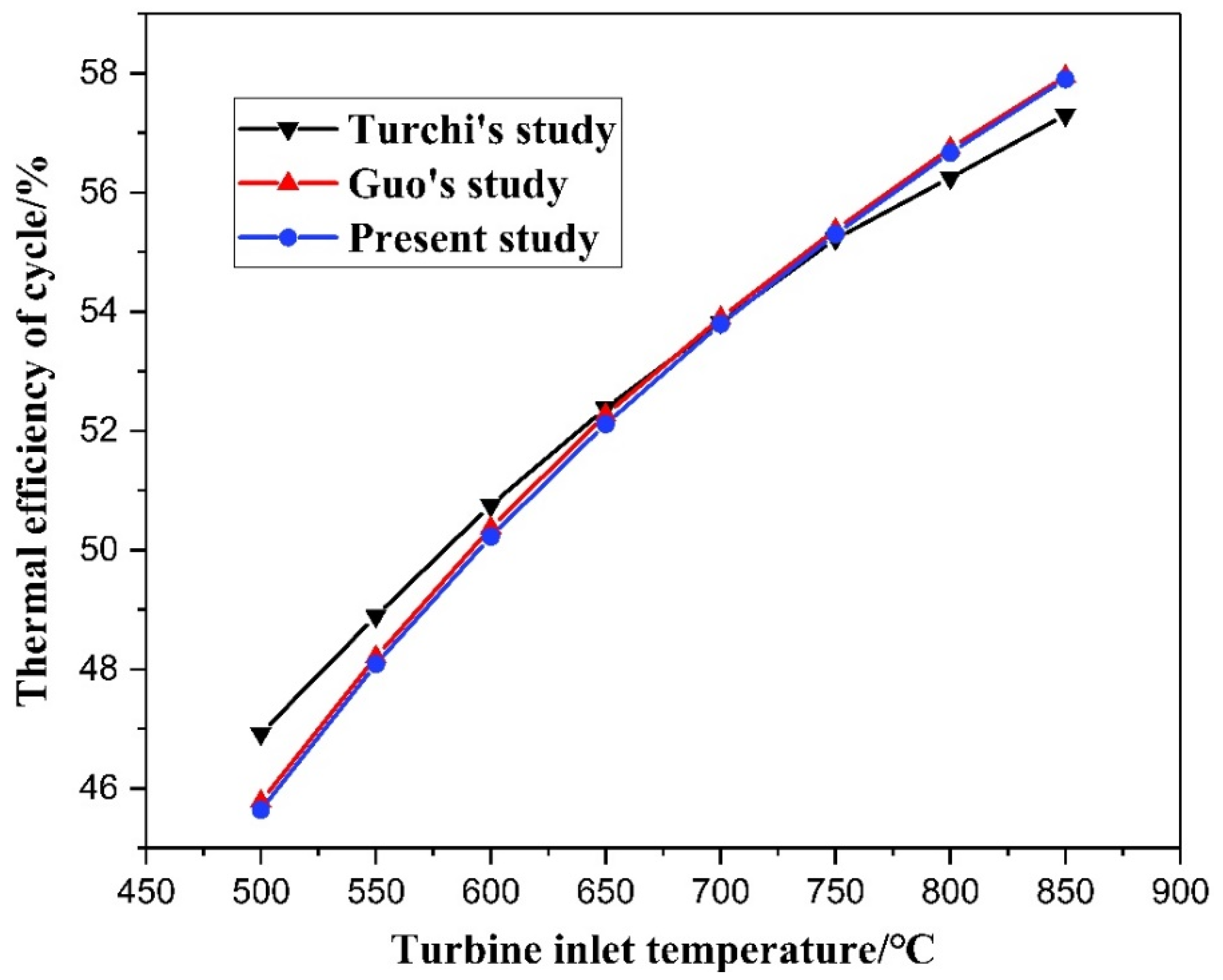
3.5. Model Validation

In this paper, the calculation model is verified by comparing it with Turchi [21] and Guo [40]. The cycle layout in those studies show a recompression re-heating cycle, and the parameters shown in

Table 3. Parameters for model validation.

Constant Parameters in the Cycle	Value	Unit
Turbine inlet pressure	25	MPa
Turbine inlet temperature	500–850	°C
Compressor inlet pressure	7.38	MPa
Compressor inlet temperature	32	°C
Re-heating pressure	16.19	MPa
Turbine efficiency	93	%
Compressor efficiency	89	%
Recuperator effectiveness	95	%

are used. The comparison of the results is shown in Figure 6, which can illustrate that the model in the present study is very consistent with that of Turchi and Guo.

4. Results and Discussion

4.1. Parameter Study

It is very important to study the influence of key parameters on system performance. Thus, the parameter study, including effects of turbine inlet temperature and pressure, compressor inlet temperature, and pressure on specific work, overall efficiency, and cost of core equipment is performed. In order to make a fair comparison of the three types of cycles, and considering that the solar collector used is the parabolic trough solar collector, the basic condition is shown in

Table 4. Base condition for the parameter study.

Constant Parameters in the Cycle	Value	Unit
Temperature of environment	25	°C
Isentropic efficiency of turbine	85	%
Isentropic efficiency of compressor	80	%
End temperature difference in regenerator	10	°C
Direct solar radiation intensity	1000	W/m2
Recuperator effectiveness	95	%
Turbine inlet pressure	18	MPa
Turbine inlet temperature	350	°C
Compressor inlet pressure	8.0	MPa
Compressor inlet temperature	35	°C

.

Figure 7, Figure 8 and Figure 9 show the results of the parameter study on three cycle layouts. It should be noted that the heat exchange efficiency and working temperature of the parabolic trough solar collector are low, so overall efficiency of the three cycles are low, but the actual thermal cycle efficiency of them is about 25%–30%, while the turbine inlet temperature is 350 °C. In contrast, due to the limitation of the inlet temperature of the turbine, the actual thermal efficiency of ORC Rankine cycle is basically 20%-24% [41], which is lower than the actual thermal efficiency of the S-CO₂ cycles in this study. However, for the steam Rankine cycle, the overall efficiency is 24.5% when the turbine inlet temperature is 390 °C, which is higher than the S-CO₂ cycles in this study [42]. However, S-CO₂ cycles have fewer phase changes, so it needs no condenser arrangement and can reduce the number of valves, resulting in fewer total area and cost.

Figure 7 illustrates the effects of the above parameters on a simple recuperated cycle, respectively. Specific work, overall efficiency, and cost of core equipment increase with the rising turbine inlet temperature and pressure, as shown in Figure 7a,b. Figure 7c shows that the specific work decreases and cost of core equipment increases with the rise of the compressor inlet temperature due to the increase of compression work. However, the overall efficiency changes tinily, and then decreases as the compressor inlet temperature rises. Figure 7d is the influence of compressor inlet pressure on specific work, overall efficiency, and cost of core equipment. In the range of compressor inlet pressure, there will be extreme values of specific work and overall efficiency due to pseudo critical pressure.

Figure 8 illustrates the effects of the same parameters on the intercooling cycle respectively. Similar to the simple recuperated cycle, the relevant parameters generally increase as the turbine inlet temperature and pressure rises, which is shown in Figure 8a,b. It can be seen from Figure 8c that the cost of core equipment increases while specific work and overall efficiency decreases as the compressor inlet temperature rises. Figure 8d shows that overall efficiency and the specific work firstly increases as the compressor inlet pressure rises, and then decreases.

Figure 9 illustrates the effects of the same parameters on the recompression cycle, respectively. The change trend shown in Figure 9a–c are, basically, similar to the above two cycles, the only difference is that with the turbine inlet pressure rising, the increase speed of overall efficiency slows down. For the recompression cycle layout, overall efficiency and the specific work have a similar trend—to intercool the cycle with the rise of the compressor inlet pressure.

It can be seen from the results of the parameter study that the performance of the system is obviously affected by several parameters, and the influence of the compressor inlet temperature and pressure on performance are not simply monotone. Furthermore, using the same parameters set cannot maximize the specific work, overall efficiency, and minimize the cost of core equipment at the same time.

Moreover, the parameter study is difficult to correct and complete comparison between the cycle layouts because the analysis is calculated on the base condition. Therefore, it is necessary to perform multi-objective optimization and then compare the various cycle layouts.

4.2. Multi-Objective Optimization

In the previous section, we analyzed three performance parameters as specific work, overall efficiency, and cost of core equipment. For the S-CO₂ power cycle using solar energy, we were concerned about the net power—that the system could provide in the operation condition and the purchase cost of the system during the construction period. Thus, we chose the specific work and cost of core equipment during the optimization.

The objective of this study is to maximize the system net power and, in the meantime, minimize the investment cost.

Table 5. Set of decision variables and their range of variation.

Decision Variables	Range	Unit
Turbine inlet temperature	300–400	°C
Turbine inlet pressure	14–20	MPa
Compressor inlet pressure	7.5–9.5	MPa
Compressor inlet temperature	32–45	°C

gives the selected decision variables and its corresponding range.

The multi-objective optimization process is conducted with GA and the solver is MATLAB R2019b. The basic steps of genetic algorithm include coding, population initialization, fitness calculation, evolution (composed of selection, crossover, mutation), and iteration. In this work, the optimal setting of the GA algorithm is set to 50 for each generation of population at population initialization. Moreover, when the genetic algebra reaches 400, the calculation terminates, which can limit the number of iterations. The reason for this set is—we find that if the total number of calculations is less than this set, the results have much more randomness. When we chose these two parameters, the results of the multiple calculations had little change. Based on the three research cycles, the optimal Pareto fronts are presented in Figure 10, Figure 11 and Figure 12.

The optimal Pareto fronts show the trade-off between the cost of core equipment and the specific work under the optimum conditions. In addition, the scatter points in the figures are for each working condition and the optimization results of the calculation process. It is worth noting that there is a significant discontinuity in the Pareto optimization results in Figure 10, Figure 11 and Figure 12, especially when the specific work is low. The results from the algorithm and its capability of evolution can first analyze the first-generation cluster. Then, the algorithm keeps the representative individuals and proceeds. These representative individuals are selected from the clusters of best performance. When a series of results barely improve through optimization, a few elite individuals are further selected. Hence, this results in a smaller portion of the global Pareto front with fewer solutions condensing. However, this discontinuity has no effect on the analysis of the results and the comparison of the systems.

From Figure 10, the values of the optimization objectives for a simple recuperated cycle increased from 30 to 70 kW/kg for specific work, and from $155,000 to $210,000 USD for the cost of core equipment. Outside these ranges, we can conclude that—for the poorer performance solutions—the cost cannot reduce, or, due to thermodynamic limits, the system net power cannot increase.

Figure 11 presents the result of intercooling configuration. The values of the optimization objectives extend between 27 and 65 kW/kg for specific work and from $255,000 to $365,000 USD for the cost of core equipment. Compared with a simple recuperated cycle, the economic cost of the intercooling cycle is too expensive and the specific work has not been significantly improved. Moreover, it can be concluded that the optimization result of the range of cost of the core equipment in the intercooling cycle is larger than the optimization result range of the simple recuperated cycle. Hence, for this cycle, reasonable selection of system operation parameters is more important for the cost reason.

Figure 12 shows the optimization result of the recompression cycle. The values of the optimization objectives extend between 25 and 50 kW/kg for specific work and from $270,000 to $370,000 USD for the cost of core equipment. Compared with the simple recuperated cycle, the economic cost and the specific work of the recompression cycle and intercooling cycle are lack of competitiveness.

To keep things straight, the optimized Pareto set of three cycles are compared and shown in Figure 13. These cycle layouts are compared in the coordinate system of “cost of core equipment and specific work”. In the “cost of core equipment and specific work” coordinate system, the location closer to the lower right corner means more excellent performance. Although the device cost of this study is not fully calculated and the actual system payback period cannot be calculated correctly. However, from Figure 13, we can still see that the simple recuperated cycle has obvious advantages over the recompression cycle and intercooling cycle after optimization. In detail, under the same level of specific work, the cost of the core equipment of the simple recuperated cycle is lower than that of the recompression cycle and intercooling cycle, which can be clearly seen in the figure.

However, a previous study has shown that when the central receiver tower with heliostat field is used, the intercooling cycle and recompression cycle will achieve greater efficiency [23]. The reason for this phenomenon may be that the temperature of the S-CO₂ entering turbine is too low when using the parabolic trough solar collector. Because of this bottleneck, the complex system structure cannot produce an obvious advantage of specific work while the increase of its cost is significant. Moreover, complex cycle structures are often used in superposition, such as recompression, intercooling, and reheating. Thus, they are more suitable for higher temperature scenarios.

4.3. Sensitivity Analysis of a Typical Result

Through the description in Section 4.2, it can be found that the simple recuperated cycle has incomparable advantages in S-CO₂ power generation cycles using solar energy by a parabolic trough solar collector. Even though it is difficult to carry out a complete investment recovery analysis through the specific work and the cost of core equipment, we can still conclude that the simple recuperated cycle has the best economy among the three cycle types. Therefore, a typical optimization result in the simple recuperated cycle is selected for sensitivity analysis in this section.

The parameters in typical optimization results selected are shown in

Table 6. System parameters in typical optimization results.

Variables	Value	Variables	Value
Turbine inlet temperature	382.76 °C	Cost of core equipment	183.98k$
Turbine inlet pressure	17.15 MPa
Compressor inlet pressure	8.82 MPa	Specific work	50.69 kW·kg−1
Compressor inlet temperature	32.35 °C

, and the rest of the parameters of the system are shown in Table 4.

First, the cost of each core component is compared with histogram and cumulative proportion, as shown in Figure 14. It can be seen that the cost of turbine machinery, including turbine and compressor, is the main component of equipment cost. This is because the technology of other components in S-CO₂ power is mature, while the manufacturing of turbine machinery using S-CO₂ is relatively difficult and the cost is high. Therefore, it can be concluded that reducing the manufacturing cost of the turbine machinery can achieve higher economic benefits.

Secondly, sensitivity analysis is considered on the cost of the core equipment and specific work. Since the cost of turbine machinery accounts for the main part, and the compressor inlet temperature after optimization is rather low (which resulted in less change space), the analysis variables are mainly turbine inlet temperature, turbine inlet pressure, compressor inlet pressure, isentropic efficiency of turbine, and isentropic efficiency of the compressor. The five parameters vary by –5% and +5%. The results of the sensitivity analysis are shown in

Table 7. Sensitivity analysis results.

Variables	Value	Cost of Core Equipment/k$	Specific Work / kW·kg−1
Turbine inlet temperature	363.62 °C	182.33(–0.90%)	48.36(–4.60%)
	401.90 °C	185.57(+0.86%)	53.00(4.56%)
Turbine inlet pressure	16.29 MPa	179.40(–2.49%)	47.42(–6.45%)
	18.00 MPa	188.16(+2.27%)	53.64(+5.82%)
Compressor inlet pressure	8.38 MPa	188.54(+2.48%)	54.19(+6.90%)
	9.26 MPa	179.38(–2.50%)	47.29(–6.71%)
Isentropic efficiency of turbine	80.75%	182.77(–0.65%)	47.45(–6.39%)
	89.25%	185.17(+0.64%)	53.93(+6.39%)
Isentropic efficiency of compressor	76%	185.30(+0.72%)	49.95(–1.46%)
	84%	182.71(–0.69%)	51.37(+1.34%)

.

Through the sensitivity analysis, it can be found that most of the changes of these variables only affect the cost of a single component, so the overall cost is not sensitive to them. The specific work is still sensitive to these variables. For the cost of core equipment, the change of pressure will cause great fluctuation; this is because the change of pressure affects the performance of two types of turbomachinery (turbine and compressor), resulting in a great change of cost. As for the specific work, in addition to the compressor efficiency, the influence of other parameters is more obvious, which is also reflected in Section 4.1. The influence of the system design parameters on the cost of core equipment is less than that on the specific work of the system. Therefore, in the actual process, more consideration should be given to the thermal performance of the system regarding the selection of system parameters, and the structural optimization and layout optimization of components should be adopted to reduce the system cost.

5. Conclusions

In this paper, a preliminary analysis and systematic comparison of three S-CO₂ power generation cycles using solar energy by the parabolic trough solar collector are studied. Firstly, the effects of the turbine inlet temperature and pressure, compressor inlet temperature and pressure on specific work, overall efficiency, and cost of core equipment of S-CO₂ Brayton cycles are discussed. After that, multi-objective optimizations are studied, taking the specific work and the cost of core equipment as the objectives. The optimized Pareto sets obtained through multi-objective optimizations are used to compare different cycle layouts. The main conclusion follows:

(1)

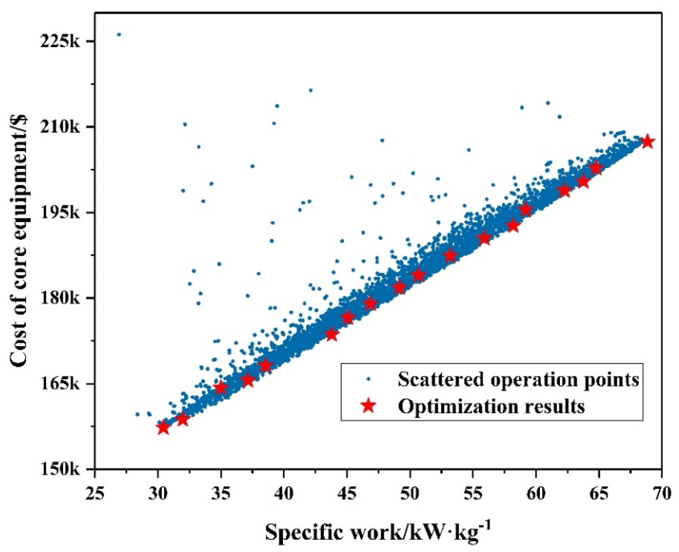
It results in an optimal specific work ranging between 30 and 70 kW/kg, and optimal cost of core equipment ranging between $155,000 and $210,000 USD for the simple recuperated cycle. The values of the optimization objectives extend between 27 and 65 kW/kg for specific work and between $255,000 and $365,000 USD for cost of core equipment in the intercooling cycle. Moreover, the values of the optimization objectives extend between 25 and 50 kW/kg for specific work and from $270,000 and $370,000 USD for cost of core equipment in the recompression cycle.

(2)

The simple recuperation cycle layout shows more excellent performance than the intercooling cycle layout and the recompression cycle layout in terms of cost, while the advantage in specific work of the intercooling cycle layout and the recompression cycle layout is not obvious.

(3)

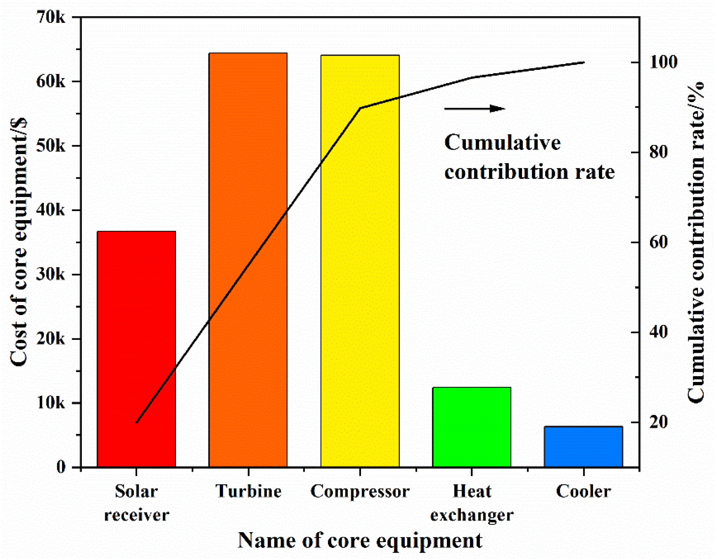
The sensitivity analysis of a typical optimization result of a simple regeneration cycle shows that the change of parameters have little influence on the cost of core equipment and much influence on specific work.

(4)

Through this study, it can be found that the turbine inlet temperature is low using a parabolic trough solar collector, and the complex SCO₂ Brayton cycles are not dominant.

(5)

The preliminary analysis and systematic comparison in this study can be useful in selecting cycle layout using solar energy by a parabolic trough solar collector when there are requirements for the specific work and the cost of core equipment. Moreover, it can also provide reference for the comparison and selection of other cycle types.

In future studies, a comprehensive analysis of investments profitability based on more accurate cost accounting methods will obtain more practical system comparison results. For components, improving the manufacturing level of turbine machinery and reducing its cost will make the S-CO₂ power generation cycles more competitive.

References

1. Mellit, A.; Massi, P.A.; Ogliari, E.; Leva, S.; Lughi, V. Advanced Methods for Photovoltaic Output Power Forecasting: A Review. Appl. Sci. 2020, 10, 487. [Google Scholar] [CrossRef] [Green Version]
2. Cucchiella, F.; D’Adamo, I.; Gastaldi, M. A profitability assessment of small-scale photovoltaic systems in an electricity market without subsidies. Energ. Convers. Manag. 2016, 129, 62–74. [Google Scholar] [CrossRef]
3. Fthenakis, V.; Raugei, M. Environmental life-cycle assessment of photovoltaic systems. In The Performance of Photovoltaic (PV) Systems; Pearsall, N., Ed.; Woodhead Publishing: Cambridge, UK, 2017; pp. 209–232. [Google Scholar]
4. Li, L.; Sun, J.; Li, Y. Prospective fully-coupled multi-level analytical methodology for concentrated solar power plants: General modelling. Appl. Therm. Eng. 2017, 118, 171–187. [Google Scholar] [CrossRef]
5. Qiu, Y.; He, Y.L.; Cheng, Z.D.; Wang, K. Study on optical and thermal performance of a linear Fresnel solar reflector using molten salt as HTF with MCRT and FVM methods. Appl. Energy 2015, 146, 162–173. [Google Scholar] [CrossRef]
6. Du, B.C.; He, Y.L.; Zheng, Z.J.; Cheng, Z.D. Analysis of thermal stress and fatigue fracture for the solar tower molten salt receiver. Appl. Therm. Eng. 2016, 99, 741–750. [Google Scholar] [CrossRef]
7. ACCIONA. Nevada Solar One. Available online: http://www.acciona.us/projects/energy/concentrating-solar-power/nevada-solar-one/ (accessed on 1 January 2017).
8. Fernández-García, A.; Zarza, E.; Valenzuela, L.; Pérez, M. Parabolic-trough solar collectors and their applications. Renew. Sustain. Energy Rev. 2010, 14, 1695–1721. [Google Scholar] [CrossRef]
9. Cayer, E.; Galanis, N.; Desilets, M.; Nesreddine, H.; Roy, P. Analysis of a carbon dioxide transcritical power cycle using a low temperature source. Appl. Energ. 2009, 86, 1055–1063. [Google Scholar] [CrossRef]
10. Price, H.; Lüpfert, E.; Kearney, D.; Zarza, E.; Cohen, G.; Gee, R.; Mahoney, R. Advances in parabolic trough solar power technology. J. Energ. Eng. 2002, 124, 109–125. [Google Scholar] [CrossRef]
11. Usman, M.; Imran, M.; Yang, Y.; Lee, D.H.; Park, B.-S. Thermo-economic comparison of air-cooled and cooling tower based Organic Rankine Cycle (ORC) with R245fa and R1233zde as candidate working fluids for different geographical climate conditions. Energy 2017, 123, 353–366. [Google Scholar] [CrossRef]
12. Mecheri, M.; Le Moullec, Y. Supercritical CO2 Brayton cycles for coal-fired power plants. Energy 2016, 103, 758–771. [Google Scholar] [CrossRef]
13. Singh, R.; Miller, S.A.; Rowlands, A.S.; Jacobs, P.A. Dynamic characteristics of a direct-heated supercritical carbon-dioxide Brayton cycle in a solar thermal power plant. Energy 2013, 50, 194–204. [Google Scholar] [CrossRef]
14. Hiroaki, T.; Niichi, N.; Masaru, H.; Ayao, T. Forced convection heat transfer to fluid near critical point flowing in circular tube. Int. J. Heat Mass Transfer. 1971, 14, 739–750. [Google Scholar] [CrossRef]
15. Monje, B.; Sanchez, D.; Savill, M.; Pilidis, P.; Sanchez, T. A Design Strategy for Supercritical CO2 Compressors; American Society Mechanical Engineers: New York, NY, USA, 2014. [Google Scholar]
16. Kim, Y.M.; Kim, C.G.; Favrat, D. Transcritical or supercritical CO2 cycles using both low- and high-temperature heat sources. Energy 2012, 43, 402–415. [Google Scholar] [CrossRef]
17. Osorio, J.D.; Hovsapian, R.; Ordonez, J.C. Dynamic analysis of concentrated solar supercritical CO2-based power generation closed-loop cycle. Appl. Therm. Eng. 2016, 93, 920–934. [Google Scholar] [CrossRef]
18. Valdes, M.; Abbas, R.; Rovira, A.; Martin-Aragon, J. Thermal efficiency of direct, inverse and SCO2 gas turbine cycles intended for small power plants. Energy 2016, 100, 66–72. [Google Scholar] [CrossRef]
19. De la Calle, A.; Bayon, A.; Hinkley, J.; Pye, J. System-level simulation of a novel solar power tower plant based on a sodium receiver, PCM storage and sCO2 power block. AIP Conf. Proc. 2018, 2033, 210003. [Google Scholar]
20. Binotti, M.; Astolfi, M.; Campanari, S.; Manzolini, G.; Silva, P. Preliminary assessment of SCO2 cycles for power generation in CSP solar power plants. Appl. Energ. 2017, 204, 1007–1017. [Google Scholar] [CrossRef]
21. Turchi, C.S.; Ma, Z.; Neises, T.W.; Wagner, M.J. Thermodynamic study of advanced supercritical carbon dioxide power cycle for concentrating solar power. J. Sol. Energy Eng. 2013, 135, 041007. [Google Scholar] [CrossRef]
22. Padilla, R.V.; Too, Y.C.S.; Benito, R.; Stein, W. Exergetic analysis of supercritical CO2 Brayton cycles integrated with solar central receivers. Appl. Energ. 2015, 148, 348–365. [Google Scholar] [CrossRef]
23. Chapman, D.J.; Arias, D.A. An Assessment of the Supercritical Carbon Dioxide Cycle for Use in a Solar Parabolic Trough Power Plant. In Proceedings of the Supercritical CO2 Power Cycle Symposium, New York, NY, USA, 29–30 April 2009. [Google Scholar]
24. Singh, R.; Rowlands, A.S.; Miller, S.A. Effects of relative volume-ratios on dynamic performance of a direct-heated supercritical carbon-dioxide closed Brayton cycle in a solar-thermal power plant. Energy 2013, 55, 1025–1032. [Google Scholar] [CrossRef] [Green Version]
25. Wang, K.; Li, M.J.; Guo, J.Q.; Li, P.W.; Liu, Z.B. A systematic comparison of different S-CO2 Brayton cycle layouts based on multi-objective optimization for applications in solar power tower plants. Appl. Energ. 2018, 212, 109–121. [Google Scholar] [CrossRef]
26. Vasquez Padilla, R.; Soo Too, Y.C.; Benito, R.; McNaughton, R.; Stein, W. Multi-objective thermodynamic optimisation of supercritical CO2 Brayton cycles integrated with solar central receivers. Int. J. Sustain. Energy 2018, 37, 1–20. [Google Scholar] [CrossRef]
27. Ho, C.K.; Carlson, M.; Garg, P.; Kumar, P. Technoeconomic Analysis of Alternative Solarized s-CO2 Brayton Cycle Configurations. J. Solar Energy Eng. 2016, 138, 051008. [Google Scholar] [CrossRef]
28. Feher, E.G. The supercritical thermodynamic power cycle. Energ. Convers. 1968, 8, 85–90. [Google Scholar] [CrossRef]
29. Ahn, Y.; Bae, S.J.; Kim, M.; Cho, S.K.; Baik, S.; Lee, J.I.; Cha, J.E. Review of supercritical CO2 power cycle technology and current status of research and development. Nucl. Eng. Technol. 2015, 47, 647–661. [Google Scholar] [CrossRef] [Green Version]
30. Moisseytsev, A.; Sienicki, J.J. Investigation of alternative layouts for the supercritical carbon dioxide Brayton cycle for a sodium-cooled fast reactor. Nucl. Eng. Des. 2009, 239, 1362–1371. [Google Scholar] [CrossRef]
31. Calle, A.D.L.; Bayon, A.; Too, Y.C.S. Impact of ambient temperature on supercritical CO2 recompression Brayton cycle in arid locations: Finding the optimal design conditions. Energy 2018, 153, 1016–1027. [Google Scholar] [CrossRef]
32. Wang, X.; Li, X.; Li, Q.; Liu, L.; Liu, C. Performance of a solar thermal power plant with direct air-cooled supercritical carbon dioxide Brayton cycle under off-design conditions. Appl. Energy 2020, 261, 114359. [Google Scholar] [CrossRef]
33. Guo, J.; Huai, X.; Cheng, K. The comparative analysis on thermal storage systems for solar power with direct steam generation. Renew. Energ. 2018, 115, 217–225. [Google Scholar] [CrossRef]
34. Gnielinski, V. New equations for heat mass transfer in turbulent pipe and channel flows. Int. Chem. Eng. 1976, 16, 359–368. [Google Scholar]
35. Ratzel, A.; Hickox, C.; Gartling, D. Techniques for reducing thermal conduction and natural convection heat losses in annular receiver geometries. J. Sol. Energ-T. Asme 1979, 101, 108–113. [Google Scholar] [CrossRef]
36. Swinbank, W.C. Long-wave radiation from clear skies. Q. J. Roy. Meteor. Soc. 1963, 89, 339–348. [Google Scholar] [CrossRef]
37. Dostal, V.; Driscoll, M.J.; Hejzlar, P. A supercritical carbon dioxide cycle for next generation nuclear reactors. Mass. Inst. Technol. 2004, 154, 265–282. [Google Scholar]
38. Henchoz, S.; Buchter, F.; Favrat, D.; Morandin, M.; Mercangoz, M. Thermoeconomic analysis of a solar enhanced energy storage concept based on thermodynamic cycles. Energy 2012, 45, 358–365. [Google Scholar] [CrossRef]
39. Yoon, S.H.; Kim, J.H.; Hwang, Y.W.; Kim, M.S.; Min KKim, Y. Heat transfer and pressure drop characteristics during the in-tube cooling process of carbon dioxide in the supercritical region. Int. J. Refrig. 2003, 26, 857–864. [Google Scholar] [CrossRef] [Green Version]
40. Guo, J.Q.; Li, M.J.; He, Y.L.; Xu, J.L. A study of new method and comprehensive evaluation on the improved performance of solar power tower plant with the CO2-based mixture cycles. Appl. Energ. 2019, 256, 113837. [Google Scholar] [CrossRef]
41. He, Y.L.; Mei, D.H.; Tao, W.Q.; Yang, W.W.; Liu, H.L. Simulation of the parabolic trough solar energy generation system with Organic Rankine Cycle. Appl. Energy 2012, 97, 630–641. [Google Scholar] [CrossRef]
42. Al-Sulaiman, F.A. Energy and sizing analyses of parabolic trough solar collector integrated with steam and binary vapor cycles. Energy 2013, 58, 561–570. [Google Scholar] [CrossRef]
Figure 1. Configuration of the simple recuperated cycle.
Applsci 10 03123 g001
Figure 2. Configuration of the intercooling cycle.
Applsci 10 03123 g002
Figure 3. Configuration of the recompression cycle.
Applsci 10 03123 g003
Figure 4. The energy balance for the solar receiver.
Applsci 10 03123 g004
Figure 5. The nodalization of the heat exchanger.
Applsci 10 03123 g005
Figure 6. Results of the present study compared to data from Turchi’s and Guo’s studies.
Applsci 10 03123 g006
Figure 7. Effects of the turbine inlet temperature (a), turbine inlet pressure (b), compressor inlet temperature (c), and compressor inlet pressure (d) on specific work, overall efficiency, and cost of core equipment (simple recuperated cycle).
Applsci 10 03123 g007
Figure 8. Effects of the turbine inlet temperature (a), turbine inlet pressure (b), compressor inlet temperature (c), and compressor inlet pressure (d) on specific work, overall efficiency, and cost of core equipment (intercooling cycle).
Applsci 10 03123 g008
Figure 9. Effects of the turbine inlet temperature (a), turbine inlet pressure (b), compressor inlet temperature (c), and compressor inlet pressure (d) on specific work, overall efficiency, and cost of core equipment (recompression cycle).
Applsci 10 03123 g009
Figure 10. Optimization result of the simple recuperated cycle.
Applsci 10 03123 g010
Figure 11. Optimization result of the intercooling cycle.
Applsci 10 03123 g011
Figure 12. Optimization result of recompression cycle.
Applsci 10 03123 g012
Figure 13. Comparison of Pareto sets for three cycles.
Applsci 10 03123 g013
Figure 14. Comparison of core equipment cost.
Applsci 10 03123 g014