Article

Practical Adaptive Sliding-Mode Control Approach for Precise Tracking of Robot Manipulators

1
Agency for Defense Development (ADD), The 1st R&D Institute—5th Directorate, Daejeon 34186, Korea
2
Electronics and Telecommunications Research Institute (ETRI), Smart Mobility Research Section, Daegu 42994, Korea
*
Author to whom correspondence should be addressed.
Appl. Sci. 2020, 10(8), 2909; https://doi.org/10.3390/app10082909
Submission received: 27 March 2020 / Revised: 16 April 2020 / Accepted: 20 April 2020 / Published: 23 April 2020

Abstract

:
We present a practical adaptive sliding-mode control approach, namely, the strong and stable adaptive sliding-mode control (SS-ASMC), in this paper. There is a significant effort towards addressing the technical challenges associated with the switching gains with two adaptive laws, which are called parent and child adaptive laws. A parent adaptive law helps achieve strong switching gains through fast adaptation rate when sliding variable moves away from the sliding manifold. A child adaptive law updates the parameter of the parent adaptive law, which helps to achieve the switching gains with fast and stable adaptation rate in the vicinity of the sliding manifold. Such switching gains with two adaptive laws provide remarkably precise tracking performance while enhancing the robustness. Besides, to yield desirable closed-loop poles and simplicity of control approach structure, the proposed SS-ASMC approach employs a combination of time-delayed estimation and pole-placement method, which makes it unnecessary to have a rather complete system dynamics. It is shown by the bounded-input-bounded-output stability through the Lyapunov approach, and thus the tracking errors are also proved to be uniformly ultimately bounded. The effectiveness of the proposed SS-ASMC approach is illustrated in simulations with robot manipulators, which is compared with that of the existing control approaches.

1. Introduction

Robot manipulators work for practicing engineers carrying out repetitive and complex tasks. Especially, they help human works requiring high precision in a variety of industrial tasks. To perform these time-consuming, e.g., repetitive and complex tasks, and precise tasks, increasing attention is being given to the tracking control of robot manipulators. However, given that the robot manipulators suffer from nonlinearity, uncertainties, and disturbances in their dynamics, there exists difficulty in establishing suitable tracking performance. For this reason, there has been tremendous progress in the development of various control strategies for the robot manipulators over the past few years.
Computed torque control approaches [1,2] have been introduced for improving the tracking performance, and employ a nominal system model for estimating a dynamics behavior of the system. They can compensate the nonlinear dynamics by using the system model and therefore are known as the effective motion control strategies in the robot manipulators. However, implementation of these control approaches is highly complicated and computationally demanding because of the calculation of the nonlinear system model, while not attaining the optimal control parameters. For this reason, there may exist poor tracking performance in the robot manipulators. Therefore, there is still room for system instability. Linear quadratic regulator (LQR) control approaches [3,4] have been studied to be designed in the optimal parameters. These control approaches have a simple structure and therefore offer ease-of-use in the robot manipulators. However, the LQR control approaches may deteriorate the tracking performance because they may degrade the robustness when the undesirable side effects, e.g., internal disturbances and unstructured/structured uncertainties, occur in the robot manipulators. H control approaches [5,6] have been developed to overcome the above-mentioned problems. They have provided a result in increasing the robustness against the internal disturbances. However, given that H control approaches depend on feasible sets of solutions, i.e., optimal parameters, to the strict groups of linear matrix inequality and Riccati equation, they construct a class of complex control structure. Besides, all control approaches described above should be required in establishing an exact mathematical system model for the robot manipulators. Unfortunately, it is impossible to obtain the exact system model in real robot manipulators. Furthermore, they require the linearization method so that the requirement of prior system information is indisputable, and they are only governed by all of the linear subsystems at each operating point. To summarize, as a practical problem under the occurrence of unpredictable system uncertainties, they may still face a problem in achieving the enhanced robustness against undesired side effects, including parameter variations and external disturbances.
Conventional sliding-mode control (SMC) approaches have been designed to remedy the above-mentioned problems. They have mainly obtained much attention for their enhanced robustness even in the presence of a significant class of uncertainties and disturbances. However, the conventional SMC approaches require switching gains with large positive constants, yielding the chattering in the sliding surface which may excite high-frequency oscillation [7,8]. They produce a result in limiting the life cycle of the robot manipulators due to wear of actuators. This is why the conventional SMC approaches are not used well in real robot manipulators [9]. To avoid these problems, the boundary-layer SMC approaches [10,11] have been employed as a way to replace the signum function which is typically discontinuous function in the property of the conventional SMC. In other words, given that these control approaches are addressed by the continuous function, i.e., saturation function, they can avoid a major concern in the practical implementation of the conventional SMC. However, the boundary-layer SMC approaches still have the limitation that they require information about the upper bound on the uncertain terms. The SMC approaches with low-pass filter [12,13] have been developed as another countermeasure against the chattering. Their switching gains depend on the system state that can be obtained while employing the low-pass filter. Therefore, these control approaches do not invite any complexity in the control design for avoiding the chattering. However, it may be hard to achieve the desired tracking performance because the overestimated switching gains are consistently required for suppressing the upper bound in the presence of significantly large disturbances.
Conventional adaptive sliding-mode control (ASMC) approaches [14,15,16] have been designed to alleviate the above-mentioned problems while using time-varying switching gains with the adaptive laws. An ASMC approach [14] has been based on the Lyapunov theory, which is further addressed by input coefficient matrices and unknown system. Although its switching gains are monotonically increased to suppress the maximum uncertainty bound, they are never decreased due to its control structure. For this reason, it may cause the chattering on the sliding surface, which may result in the system instability. To solve this problem, an ASMC approach [15] has been introduced by using an adaptive law that can adjust the switching gains appropriately according to the magnitude of the sliding variable. However, this control approach has been limited to the control in the single-input single-output system. Its property is not able to eliminate the dynamic coupling effects in the joints of the robot manipulators. Since then, an ASMC approach [16] has overcome such a monotonic nature of the switching gains in the multi-input multi-output system. However, if this control approach requires the large switching gains for achieving fast convergence rate, it may cause the high-frequency dynamics because of the switching gains in the slow adaptation rate. As such, there is a need for effective ASMC approaches with powerful switching gains.
An ASMC approach [17] has been first developed to be operated in the powerful switching gains, which aims at achieving fast adaptation rate at any time as the switching gains increase or decrease. Although it offers favorable tracking performance, the switching gains may be sensitive to the parameter setting for adjusting the adaptation rate near the sliding manifold. After that, another ASMC approach [18] with auxiliary parameters has been employed to alleviate the sensitivity in relation to the parameter setting. Unfortunately, it requires a time-consuming task because of a huge amount of tuning parameters. It may cause a result that the control performance is influenced by the local switching gains, not the global switching gains. An ASMC approach [19] has been introduced to avoid these problems in the literature, which is based on the existing ASMC approach [17] for integrating the advantages derived from the fast adaptation rate. Then, its adaptive law is composed of a combination sliding variable and exponential function so that the control input fluctuation does not occur near the sliding manifold. Given that the number of parameters can be also reduced when compared to an ASMC approach [18], it offers the potential for application to real systems. However, the adaptation rate of the switching gains is not directly influenced to the magnitude of the sliding variable while staying in the vicinity of the sliding manifold, and therefore this control approach may provide unstable switching gains temporarily because of the improper and insufficient adaptation rate. As such, even though various control approaches have been performed for the ASMC approach, there are still some limitations with regard to the adaptation rate of the switching gain. In other words, given that the existing ASMC approaches only provide a fast or a stable adaptation rate, it may not be easy for practicing engineers to achieve the favorable tracking performance without the undesirable side effects. Therefore, it is necessary to develop a more simple and practical control approach that can provide the switching gains with fast and stable adaptation rate.
In this paper, we propose a practical ASMC approach, namely, the strong and stable adaptive sliding-mode control (SS-ASMC) approach, that offers strong and stable switching gains in the large and small magnitudes of the sliding variable, respectively. There is a significant effort towards addressing the technical challenges associated with the new time-varying switching gains having two adaptive laws which is called parent and child adaptive laws. A parent adaptive law is designed to be proportional to the magnitude of the sliding variable. Therefore, the proposed SS-ASMC approach can provide strong switching gains through fast adaptation rate when causing inappropriately large sliding variables by the large negative effects, e.g., abrupt disturbances. Then, the switching gains employ the time-varying update parameters with the child adaptive law that are designed to stay on its low bound while away from the sliding manifold. These adaptive laws of the proposed ASMC guarantee that within a finite time, all of the sliding variables enter an arbitrarily small vicinity of the sliding manifold and then stay around it. On the contrary, as mentioned previously, given that the parent adaptive law is designed to be proportional to the magnitude of the sliding variable, it may provide a slow adaptation rate in the vicinity of the sliding manifold. To achieve a fast and stable adaptation rate, the time-varying update parameters with the child adaptive law are activated, which has an effect of adjusting the parameters to the switching gains of the proposed SS-ASMC approach. This is a reason why the switching gains can be quickly adjusted without making them unstable. Therefore, even though the switching gains become somewhat large to achieve precise tracking performance while guaranteeing the robustness, they are not sufficiently affected by the chattering because the adaptation rate is fast and stable owing to the child adaptive law. Further, all control approaches based on sliding-mode control are in need of an equivalent control approach and thus require the complex and exact system dynamics. However, the proposed SS-ASMC approach employs a time-delayed estimation (TDE) to solve the negative demands generating in an equivalent control approach, which can compensate uncertainties, nonlinear dynamics, and unknown disturbances in the robot manipulators. Moreover, the pole-placement (PPT) is also employed to obtain the error dynamics with the dominant pole, which helps to converge to the equilibrium point. For these reasons, the proposed SS-ASMC approach can be taken without the knowledge of the system information in the robot manipulators, which makes it unnecessary to have a rather complete system dynamics. From these benefits, the proposed method works well for simulations accompanying undesirable side effects such as the parameter variations and the abrupt disturbances. It is shown that the proposed SS-ASMC approach guarantees the bounded-input bounded-output stability through Lyapunov function, meaning the tracking errors are uniformly ultimately bounded. The effectiveness of the new time-varying switching gains in the proposed SS-ASMC approach is illustrated in simulations with robot manipulators. It turns out the proposed one has strong and stable tracking performance without the chattering, and then compared with the existing control approaches.
The remainder of this paper is organized as follows. In Section 2, we briefly introduce what the proposed SS-ASMC approach is. In Section 3, we carried out simulations with the 2-link planar robot manipulator. In Section 4, we conclude with a brief summary of this paper.

2. Proposed SS-ASMC Approach

2.1. The Dynamics of Robot Manipulator

The n-axes robot manipulator model [20,21,22] can be described as follows,
M ( q t ) q ¨ t + C ( q t , q ˙ t ) q ˙ t + g ( q t ) + f ( q t , q ˙ t ) = τ t + τ d , t
where q t = ( q 1 , t , q 2 , t , , q n , t ) n , q ˙ t = ( q ˙ 1 , t , q ˙ 2 , t , , q ˙ n , t ) n , and q ¨ t = ( q ¨ 1 , t , q ¨ 2 , t , , q ¨ n , t ) n are the joint angle, the joint angular velocity, and the joint angular acceleration, respectively. M ( q t ) n × n is the symmetric positive definite that is called the moment of inertia. C ( q t , q ˙ t ) n × n is the Coriolis matrix. g ( q t ) is the gravity matrix. f ( q t , q ˙ t ) n is the friction matrix.
Multiplying M 1 ( q t ) by both sides in Equation (1), we have
q ¨ t = M 1 ( q t ) C ( q t , q t ) q ˙ t + g ( q t ) + f ( q t , q ˙ t ) τ t τ d , t
From Equation (2), the equation in a compact and simple form yields
q ¨ t = M 1 ( q t ) C ( q t , q t ) q ˙ t + g ( q t ) + f ( q t , q ˙ t ) τ d , t + M 1 ( q t ) M ¯ 1 τ t + M ¯ 1 τ t = L t + M ¯ 1 τ t
where
L t = M 1 ( q t ) C ( q t , q t ) q ˙ t + g ( q t ) + f ( q t , q ˙ t ) τ d , t + M 1 ( q t ) M ¯ 1 τ t
where M ¯ = diag ( M ¯ 1 , M ¯ 2 , , M ¯ n ) n × n is the diagonal constant matrix to be determined later on, which is called “TDC gain”, and how to choose the TDC gain M ¯ will be introduced in Appendix A. According to the well-known assumption, it is assumed that the following property [23,24,25] holds
κ ̲ m M ( q t ) 2 κ ¯ M
for the positive constants κ ̲ m and κ ¯ M .

2.2. Control Design

The control objective of this paper is to make the joint angle q t follow the command joint angle q d , t = ( q d 1 , t , q d 2 , t , , q d n , t ) n precisely. It implies that the tracking error e t = ( e 1 , e 2 , , e n ) n , which is defined as q d , t q t , is eliminated to be achieved accurately in the tracking motion of the robot manipulator. To obtain the desired performance in tracking the trajectory for each joint of the robot manipulator, we shall employ
s t = e ˙ t + K ¯ s e t
where s t = ( s 1 , s 2 , , s n ) n is the sliding variable. K ¯ s = diag ( K ¯ s , 1 , K ¯ s , 2 , , K ¯ s , n ) n × n are the diagonal positive design parameter that is called “sliding gain”. It is noted that the sliding gain K ¯ s is directly related to the rate at which the tracking error e t converges to zero, assuming the sliding variable s t is zero.
From Equation (6), we construct the following control approach as
τ t = M ¯ L ^ t + q ¨ d , t + K ¯ s e ˙ t + K ¯ g s t = M ¯ L ^ t + q ¨ d , t + K ¯ s + K ¯ g e ˙ t + K ¯ s K ¯ g e t
where K ¯ g = diag ( K ¯ g , 1 , K ¯ g , 2 , , K ¯ g , n ) n × n is the diagonal positive design parameter. The estimation value L ^ t n can be obtained from one-sample delayed measurement of L t n , which is called time-delayed estimation (TDE), and then we have
L ^ t L t L = q ¨ t L M ¯ 1 τ t
where L is the sampling time. In other words, the smaller the sampling time L is, the higher the accuracy of estimation value in L ^ t is. As known in some papers [26,27,28], the sampling time L yields the positive effects above 100 Hz, and therefore will also be set above 100 Hz in the proposed control approach.
Substituting Equation (8) into Equation (7), we can obtain the control approach with the pole-placement term (PPT) as
τ t = M ¯ q ¨ t L + τ t L TDE + M ¯ q ¨ d , t + K ¯ s + K ¯ g e ˙ t + K ¯ s K ¯ g e t PPT .
Substituting Equation (9) into Equation (3), the error dynamics can be represented as follows,
e ¨ t + K ¯ s + K ¯ g e ˙ t + K ¯ s K ¯ g e t + E t = 0
where E t = ( E 1 , t , E 2 , t , , E n , t ) n is called “TDE error”. If we can make the TDE error E t = 0 , the tracking error e t = 0 goes to zero monotonically. Then, the sliding gain K ¯ s and the design parameter K ¯ g can be defined as the desired poles that help to adjust the convergence rate.
If the sampling time L is sufficiently small, the estimation value L ^ t can be as close to L t as possible. Unfortunately, it is impossible to achieve the estimation value L ^ t that is the same as L t because the real systems exist in the discrete-time domain, inherent state noises, hard nonlinearity, and abrupt disturbances [29]. It means that the TDE errors must be present in the real systems. To achieve the system stability while guaranteeing the upper bound of these errors, the TDC gain M ¯ should be satisfied as follows,
I M 1 ( q t ) M ¯ 2 < 1
for all t > 0 , then the TDE errors E t are always upper-bounded [27,30], i.e., E i E ¯ i * for all i = 1 , 2 , , n , where E ¯ i * is the maximum value of the TDE error E i . It means that the magnitude of the TDC gain M ¯ should be restricted, and thus Equation (9) may cause degraded tracking performance.
To suppress the TDE errors E t , we propose a practical adaptive sliding-mode control (SS-ASMC) approach that is added in Equation (7) as follows,
τ t = M ¯ q ¨ t L + τ t L + M ¯ q ¨ d , t + K ¯ s + K ¯ g e ˙ t + K ¯ s K ¯ g e t + M ¯ K ^ t s sgn ( s t )
where K ^ t s = diag ( K ^ 1 , t s , K ^ 2 , t s , , K ^ n , t s ) n × n is the diagonal positive gain to be determined for guaranteeing the system stability, called “switching gain” in this paper. The switching gain employs two adaptive laws, i.e., the parent (Equation (13)) and child (Equation (14)) adaptive laws, that are
K ^ ˙ i , t s = δ ¯ i η ^ i , t | s i , t | χ t if K ^ i , t s > 0 and s i , t 0 δ ¯ i η ^ i , t | s i , t | if K ^ i , t s = 0 or s i , t = 0
where
η ^ ˙ i , t = γ ¯ i | s i , t | if | K ^ ˙ i , t s | < μ ¯ and η ^ i , t = η ¯ i * γ ¯ i | s i , t | a χ t if | K ^ ˙ i , t s | < μ ¯ and η ̲ i * < η ^ i , t < η ¯ i * γ ¯ i | s i , t | if | K ^ ˙ i , t s | < μ ¯ and η ^ i , t = η ̲ i * 0 if | K ^ ˙ i , t s | = μ ¯
where χ t = sgn ( s t ε ¯ ) . K ^ ˙ i , t s is the parent adaptive law of the switching gain K ^ i , t s . η ^ i , t is called “update parameter” whose the derivative is defined as η ^ ˙ i , t , and then it has a upper value η ¯ i * and a lower value η ̲ i * for all i = 1 , 2 , , n . ε ¯ can determine that the switching gain K ^ t s increases or decreases. δ ¯ i and γ ¯ i can adjust the adaptation rate of the switching gain K ^ t s and the update parameter η ^ i , t , respectively. μ ¯ is set to be restricted in the adaptation rate of the switching gain K ^ t s because the excessive adaptation rate may cause the control input fluctuation making the system instability. a is also set to the positive value for the sake of changes in the update parameter η ^ i , t . The signum function sgn ( s i , t ) is defined by
sgn ( s i , t ) = 1 if s i , t 0 1 if s i , t < 0 .
As shown in Equations (13) and (14), both the parent adaptive law K ^ ˙ i , t s and the child adaptive law η ^ ˙ i , t do not require the information on the uncertain terms, which can be adjusted in accordance with the magnitude of the sliding variable. The parent adaptive law K ^ ˙ i , t s is set to be proportional to the magnitude of the sliding variable. If the sliding variables s t are far from the sliding manifold, i.e., s t ε ¯ , the adaptive law K ^ ˙ i , t s is sufficiently large for all i = 1 , 2 , , n , and therefore the switching gain K ^ t s will be increased quickly through fast adaptation rate. It provides a result that the sliding variables s t go to the sliding manifold more quickly owing to the large switching gain. As another point, it means that the sliding variables s t enter the vicinity of the sliding manifold. However, the large switching gain may cause the undesirable side effect, e.g., chattering, when the sliding variable s t stays the vicinity of the sliding manifold. To alleviate this negative effect, the boundedness ε ¯ is set to decrease the switching gain K ^ t s when s t < ε ¯ . However, the adaptation rate of the switching gains K ^ t s may be slow because it is directly proportional to the magnitude of the sliding variables. In other words, when the sliding variables s t stay in the boundedness ε ¯ , inappropriately large switching gain may still cause the chattering that generates serious problems such as wear in the motor of the robot manipulator. To handle all aspects of this matter, the proposed control approach proposes a new update parameter η ^ i , t whose derivative, i.e., η ^ ˙ i , t , can be generated when the sliding variable s t stays in the vicinity of the sliding manifold. Therefore, the update parameter η ^ i , t is asymptotically increased for decreasing the switching gain K ^ t s quickly. Then, given that the update parameter η ^ i , t can be increased to be upper-bounded, it generates a finite value which helps to avoid the excessive adaptation rate of the switching gain K ^ t s . As a result, the proposed SS-ASMC approach provides the strong and stable switching gains without the undesirable side effects, including chattering, owing to the parent adaptive law K ^ ˙ i , t s and the child adaptive law η ^ ˙ i , t .
The proposed SS-ASMC approach can be depicted with a block diagram as shown in Figure 1, which provides that the sliding variable s t enters the vicinity of the sliding manifold within a finite time t ε ¯ > 0 , as shown in Theorem 1. Then, the switching gains K ^ i , t s can be upper-bounded by the unknown positive values as in Lemma 1.
Theorem 1.
For a robot manipulator controlled by the proposed SS-ASMC approach (Equation (12)), the sliding variable s t enters the vicinity of the sliding manifold within a finite time t ε ¯ > 0 , which is guaranteed to be uniformly ultimately bounded for t > t ε ¯ as
s t 2 i = 1 n ε ¯ 2 + i = 1 n 1 δ ¯ i K ˜ i , M * 2 + i = 1 n 1 γ ¯ i η ¯ i * 2
where K ˜ i , M * is the maximum value of K ˜ i , t = E ¯ i * K ^ i , t s . The proof is given in Appendix B.
Lemma 1.
The switching gains K ^ i , t s are upper-bounded by the unknown positive values K ¯ i s , * as follows,
K ^ i , t s K ¯ i s , *
for all i = 1 , 2 , , n and t > 0 . The proof is given in Appendix C.

3. Simulation

3.1. Simulation Setup

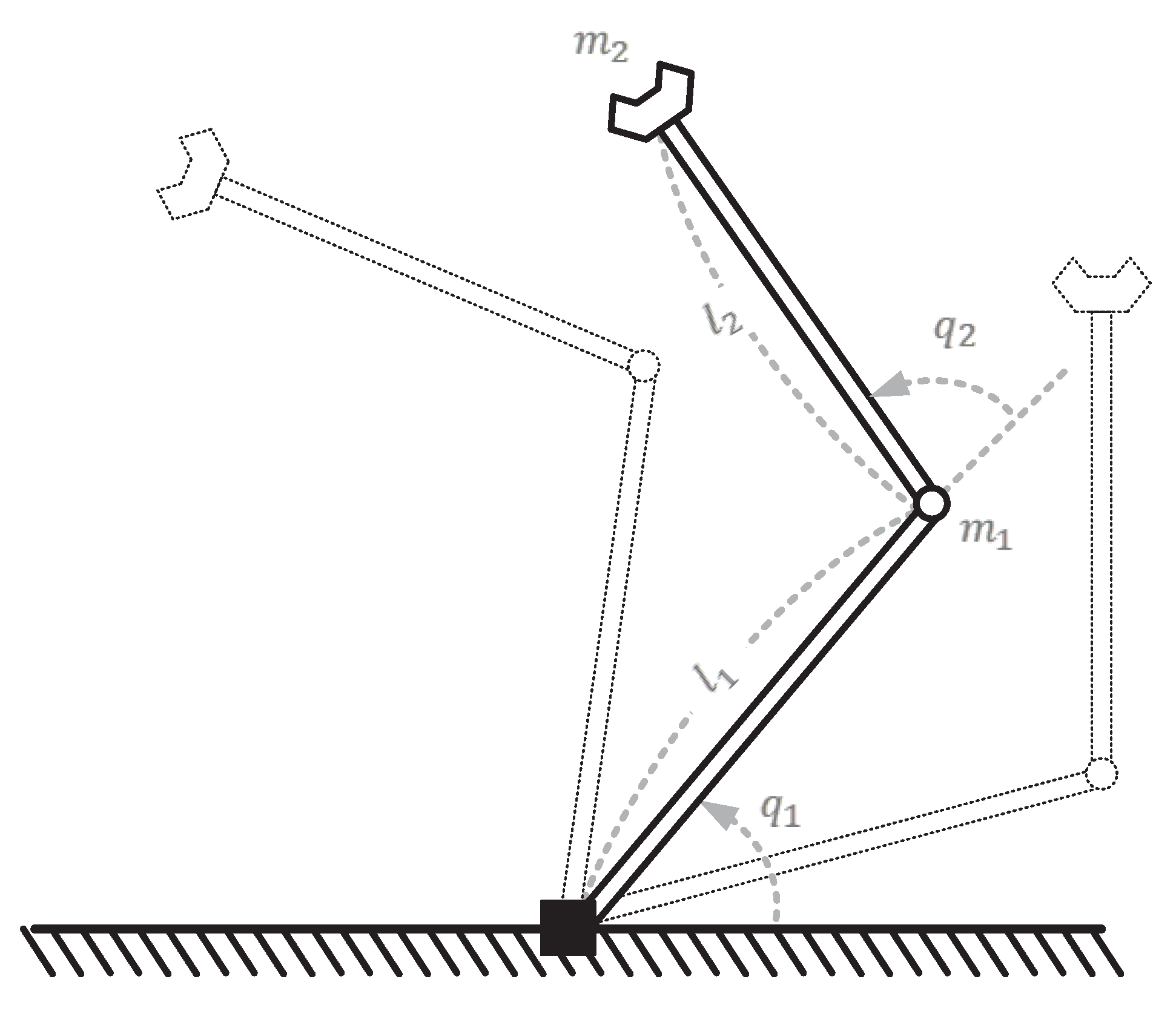
To illustrate the proposed SS-ASMC approach, a 2-link planar robot manipulator model (Figure 2) is adopted in these simulations, which is given in the Appendix D. The parameters of the proposed SS-ASMC approach are chosen as M ¯ 1 = 4 × 10 3 , M ¯ 2 = 2 × 10 3 , K ¯ s , 1 = 1 , K ¯ s , 2 = 1 , K ¯ g , 1 = 6 × 10 2 , K ¯ g , 2 = 8 × 10 2 , δ ¯ 1 = 7 , δ ¯ 2 = 22 , ε ¯ = 9 × 10 1 , γ ¯ 1 = 5 × 10 4 , γ ¯ 2 = 1 × 10 4 , a 1 = 2.5 , a 2 = 1.5 , η ¯ 1 * = η ¯ 2 * = 1 × 10 5 , η ̲ 1 * = η ̲ 2 * = 1 × 10 3 , and μ ¯ = 1 × 10 4 .

3.2. Simulation Description

The purpose of these simulations is to make the angle of joints q t in the robot manipulator catch up with the command joint angle q d , t , as shown in Figure 3. It is noted that there simulations are three points as follows.
(1)
It is well-known that the Coulomb friction accounts for nearly one-third of the maximum motor torque in the robot manipulator [31]. Moreover, the Coulomb friction leads to large TDE errors when the rotational direction of motor is changed at the moment [17]. Then, the effectiveness of the proposed SS-ASMC approach is evaluated on how to improve the nominal tracking performance through the robot manipulator.
(2)
The command angle trajectories of joints are being moving in the different phases, as shown in Figure 3, which are inherently shown in unmatched and matched disturbances, including the Coulomb friction.
  • (Unmatched disturbances)
    0.3 s, 2 s, 4.3 s, 5.8 s, 7 s, 8.3 s
  • (Matched disturbances)
    3 s, 9.5 s.
The effectiveness of the proposed SS-ASMC approach is simulated to verify its robustness against being adversely affected by such disturbances.
(3)
As an external disturbances, additional payload is applied in joint 2 of the robot manipulator, i.e., the end-effector of the robot manipulator. In this case, the robust tracking performance of the proposed SS-ASMC approach is evaluated with or without the payload.
To illustrate the effectiveness of the proposed SS-ASMC approach in these points, a
  • Time-delayed control (TDC) approach [32] and
  • Adaptive sliding-mode control (ASMC) approach [17]
are employed for comparison. The parameters of these control approaches are set in Appendix E.

3.3. Simulation Result

Figure 4 shows the update parameters that are time-varying parameters inherent in the parent adaptive law (Equation (13)). Given that the switching gains (Figure 5) can be sufficiently increased to suppress the undesirable side effects through fast adaptation rate, the update parameters move towards its low bound when the rotational direction of motor of the robot manipulator is changed at the moment. On the other hand, the update parameters are increased in the vicinity of the sliding manifold and therefore help decreasing the switching gains (Figure 5) while generating fast and stable adaptation rate. It results in producing proper switching gains without any negative effects including the chattering, as shown in Figure 5.
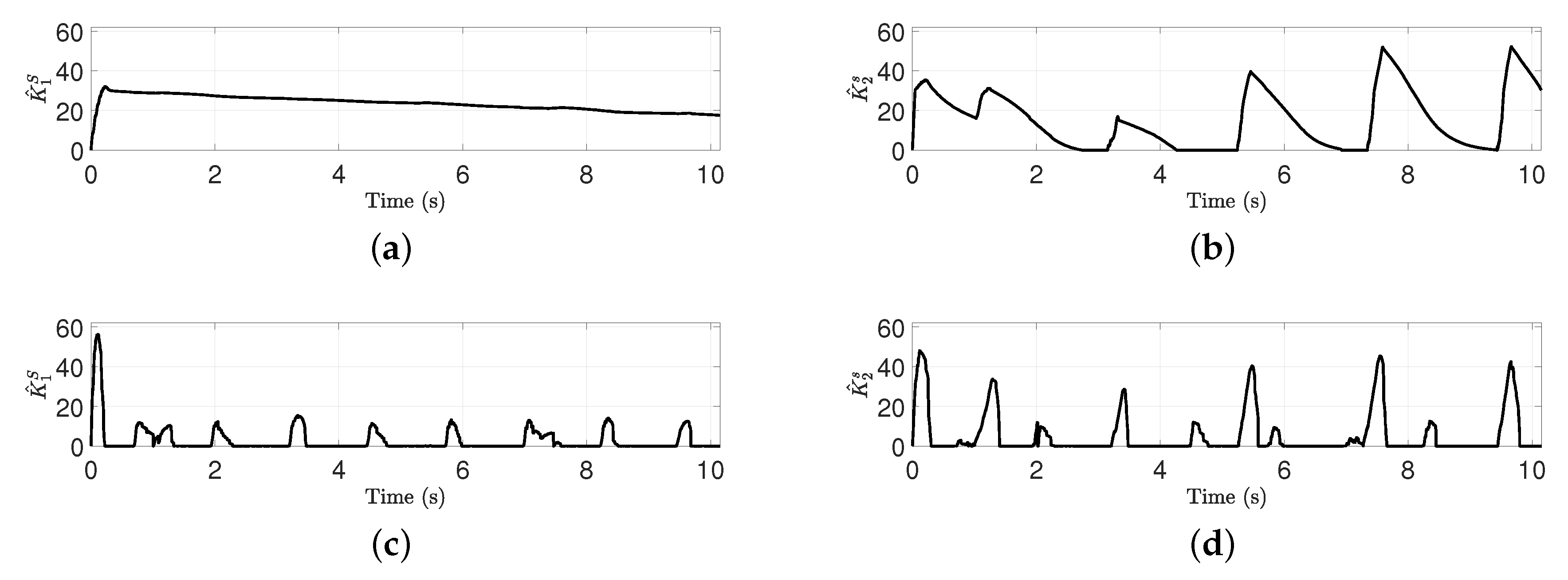
Figure 5 shows a comparison between the switching gains of the proposed SS-ASMC approach and the existing ASMC approach. As shown in Figure 5a,b, the switching gains of the proposed SS-ASMC approach are smoothly increased or decreased depending on whether the sliding variables (Figure 6) are close to the sliding manifold or not. By contrast, as shown in Figure 5c,d, the existing ASMC approach can suppress the disturbances temporarily through powerful switching gains. It seems to be superior to the tracking performance at the moment large disturbances occur because their switching gains adopt larger values than those of the proposed SS-ASMC approach. In other words, it is observed that the switching gains of the proposed SS-ASMC approach are slower when compared to those of the existing ASMC approach. However, there are residual negative effects because of the effect of inertia in the system, as shown in Figure 7. Moreover, the existing ASMC approach only depends on the convergence rate of the TDC approach in the transient sections because of the switching gains in the excessive adaptation rate. It leads to a result of the insufficient behavior in the tracking performance, as shown in Figure 7. Fortunately, the residual switching gains of the proposed SS-ASMC approach can solve the problems in the existing ASMC approach. The switching gains remaining during the decrease do not cause undesired side effects, which result in the chattering-free switching gains. Moreover, given that the switching gains of the proposed SS-ASMC approach are appropriately adjusted through fast and stable adaptation rate, it can be observed that they help to improve the nominal tracking performance in transient sections where the disturbances does not occur directly, as shown in Figure 7.
Figure 6 shows the sliding variables of the proposed SS-ASMC approach which increase temporarily when the disturbances occur. When the sliding variables leave near sliding manifold, it is strongly influenced by the switching gains of the SS-ASMC approach. Since then, the sliding variables are close to the sliding manifold. It is observed that the magnitude on the sliding variables tend to be similar to that on the tracking errors, as shown in Figure 7.
Figure 7 shows the tracking errors generated from the TDC approach, the existing ASMC approach, and the proposed SS-ASMC approach. As shown in Figure 7, the TDC approach is sufficiently affected by both unmatched/matched disturbances and the changes in the payload on the end-effector of the robot manipulator. By contrast, the existing ASMC approach improves the tracking performance against unmatched and matched disturbances. Moreover, it is not sufficiently affected by the command joint angle trajectory with and without payload on the end-effector of the robot manipulator. However, the existing ASMC approach only depends on the tracking performance of the TDC approach in the transient sections because there is no interaction between the switching gain and the control input, as in Figure 5. Furthermore, in the two control approaches described above, i.e., the TDC approach and existing ASMC approach, it can be seen that some chattering is slightly caused by the unmatched disturbances. Besides, given that the existing ASMC approach employs the switching gain with the excessive adaptation rate, its control parameters are not easy to set to be adjusted appropriately and therefore may also cause some chattering. By contrast, it is remarkably observed that the proposed SS-ASMC approach works well without undesirable side effects shown in two control approaches. Especially, ase the decreasing switching gains of the proposed SS-ASMC approach does not become zero instantaneously, they help to improve the nominal tracking performance in transient sections where the disturbances does not occur directly. Owing to fast and stable adaptation rate, it can quickly cope with undesirable side effects caused by unmatched and matched disturbances and hence can enhance the robust tracking performance. Moreover, it can be observed that the proposed one derives the natural tracking performance irrespective of payload on the end-effector of the robot manipulator. From the above results, it can be said that the proposed SS-ASMC approach offers more precise nominal and robust tracking performance than other two control approaches. The root-mean-square (RMS) tracking errors are given in Table 1.

4. Conclusions

In this paper, we proposed a practical ASMC approach with two adaptive laws, namely, the parent and child adaptive laws, in the robot manipulator. The parent adaptive law helped to provide the strong switching gains that mainly improved the tracking performance while enhancing the robustness when away from the equilibrium point. The child adaptive law helped to improve the tracking performance while achieving a fast convergence rate near the equilibrium point. The proposed SS-ASMC approach could be taken without the knowledge of the system information in the robot manipulator, which makes it unnecessary to have a rather complete system dynamics. From the synergistic effects of these properties, the proposed SS-ASMC approach provided a simple structure, but worked well for simulations with the robot manipulator accompanying undesirable side effects. The effectiveness of the proposed SS-ASMC approach was illustrated in simulations with robot manipulators, and then the proposed control approach had better tracking performance and robustness than the existing control approaches.
In the future, we believe that the proposed SS-ASMC approach will be applied to various applications.

Author Contributions

Conceptualization: J.B.; software: J.B.; data curation: J.B.; writing—original draft preparation: J.B.; writing—review and editing: J.B.; supervision: W.K.; project administration: W.K.; funding acquisition: W.K. All authors have read and agreed to the published version of the manuscript.

Funding

This project was funded by Electronics and Telecommunications Research Institute (ETRI), and is currently supported by the Korean government (20ZD1110, Development of ICT Convergence Technology for Daegu–Gyeongbuk Regional Industry).

Conflicts of Interest

The authors declare no conflict of interest.

Appendix A. How to Choose the TDC Gain

If the TDC gain M ¯ can be chosen as the diagonal elements of M ( q t ) , we can achieve the best tracking performance when operating in the system without noise. However, for real systems, given that the information of M ( q t ) is not known exactly, the TDC gain M ¯ should be tuned through the trial-and-error method. Fortunately, the stability criteria (Equation (11)) introduced in this paper implies that the smaller the TDC gain M ¯ , the easier it is to stabilize the system. Therefore, we recommend a tuning method that increases the TDC gain M ¯ at very small values.

Appendix B. Proof of Theorem

To prove the overall system stability, the Lyapunov function, denoted by V t , is defined as
V t = 1 2 s t T s t + 1 2 i = 1 n 1 δ ¯ i K ˜ i , t 2 + 1 2 i = 1 n 1 γ ¯ i η ^ i , t 2
whose the time derivative can be computed as
V ˙ t = s t T s ˙ t i = 1 n 1 δ ¯ i K ˜ i , t K ^ ˙ i , t s + i = 1 n 1 γ ¯ i η ^ i , t η ^ ˙ i , t = s t T s ˙ t + Λ 1 , t + Λ 2 , t
where
Λ 1 , t = i = 1 n 1 δ ¯ i K ˜ i , t K ^ ˙ i , t s Λ 2 , t = i = 1 n 1 γ ¯ i η ^ i , t η ^ ˙ i , t .
Substituting the time derivative of Equation (6) into Equation (A2), we have
V ˙ t = s t T q ¨ d , t q ¨ t + K ¯ s + Λ 1 , t + Λ 2 , t .
Substituting Equations (3) and (12) into Equation (A3), Equation (A3) can be represented as
V ˙ t = s t T q ¨ d , t L t M ¯ 1 τ t + K ¯ s + Λ 1 , t + Λ 2 , t = s t T E t + K ¯ g s t K ^ t s sgn ( s t ) + Λ 1 , t + Λ 2 , t
where E t = L t L t L n is the TDE error that is bounded according to Equation (11), e.g., | E i , t | E ¯ i * for all i = 1 , 2 , , n . It follows then that
V ˙ t K ¯ g s t T s t + i = 1 n | s i , t | | E i , t | K ^ i , t s + Λ 1 , t + Λ 2 , t = K ¯ g s t T s t + i = 1 n | s i , t | K ˜ i , t i = 1 n η ^ i , t | s i , t | K ˜ i , t χ t + i = 1 n 1 γ ¯ i η ^ i , t η ^ ˙ i , t .
If s t is larger than the boundedness ε ¯ , i.e., χ t = 1 , Equation (A5) can be represented as follows,
V ˙ t K ¯ g s t T s t + i = 1 n 1 γ ¯ i η ^ i , t η ^ ˙ i , t .
If | K ^ ˙ i , t s | is less than the positive value μ ¯ , Equation (A6) yields
V ˙ t K ¯ g s t T s t i = 1 n η ^ i , t | s i , t | a i = 1 n K ¯ g , i s i , t 2
when s t ε ¯ is satisfied. Equation (A7) means that the Lyapunov function V t will be decreased. Then, the time derivative of the Lyapunov function has a low-bounded value, not zero, as follows,
V ˙ t i = 1 n K ¯ g , i s i , t 2 i = 1 n K ¯ g , i ε ¯ 2
which means that the sliding variable s t reaches the boundedness ε ¯ within the finite time t ε ¯ = t 1 > 0 . In other words, given that the sliding variable s t enters the boundedness ε ¯ , we are able to have more room for the improper tracking performance if the boundedness ε ¯ can be chosen as being smaller. However, the time derivative of the Lyapunov function does not always guarantee that the sliding variable s t the boundedness ε ¯ , i.e., s t < ε ¯ . It is a reason that two terms in forth line of Equation (A5) may become positive, e.g., V ˙ t > 0 . If the sliding variable s t moves out of the boundedness ε ¯ , Equation (A8) will steer it back toward the sliding manifold. After that, the sliding variable s t arrives at the boundedness ε ¯ within the finite time t 2 > t 1 . As another point, it means that the upper bound of the sliding variable s t exists inherently.
From now, let us prove the upper bound of the sliding variable s t . To begin with, it can be seen in Equation (A1) that the Lyapunov function V t is bounded as follows,
1 2 s t 2 2 V t 1 2 s t 2 2 + 1 2 i = 1 n 1 δ ¯ i K ˜ i , t 2 + 1 2 i = 1 n 1 γ ¯ i η ^ i , t 2 .
Given that 1 2 i = 1 n 1 δ ¯ i K ˜ i , t 2 and 1 2 i = 1 n 1 γ ¯ i η ^ i , t 2 are bounded by Lemma 1 and Equation (13), Equation (A9) can be represented as
1 2 s t 2 2 V t 1 2 i = 1 n ε ¯ 2 + 1 2 i = 1 n 1 δ ¯ i K ˜ i , M * 2 + 1 2 i = 1 n 1 γ ¯ i η ¯ i * 2 .
It follows then that
s t 2 = i = 1 n ε ¯ 2 + i = 1 n 1 δ ¯ i K ¯ i , M * 2 + i = 1 n 1 γ ¯ i η ¯ i * 2
where K ˜ i , M * and η ¯ i * are the maximum values of K ˜ i , t and η ^ i , t , respectively. It is noted that the boundedness ε ¯ is dominant in relation to the magnitude of the sliding variable. From Equation (A11), the sliding variable s t is guaranteed to be bounded, which is uniformly ultimately bounded for t t ε ¯ . In Equation (A1), the sliding variable s t serves as a bounded input of the dynamics system, including the tracking error e t . It means that the tracking error e t is also bounded owing to the bounded-input-bounded-output stability [33].

Appendix C. Proof of Lemma

To prove that the upper bound of the switching gain exists, i.e., K ^ i , t s K ¯ i s , * , we assume that the Lyapunov function V t is upper-bounded as a sufficiently large V ¯ * . It follows then that
V t = 1 2 s t T s t Sliding term + 1 2 i = 1 n 1 δ ¯ i K ˜ i , t 2 Switching term + 1 2 i = 1 n 1 γ ¯ i η ^ i , t 2 Updated term V ¯ * .
Given that the updated term is bounded by Equation (13), we consider that one of them, i.e., sliding term or switching term, should be sufficiently large. To begin with, if the sliding term is sufficiently large, then the time derivative of the Lyapunov function V t becomes negative owing to Equation (A8). Next, we consider that the switching term is sufficiently large. Then, the time derivative of the Lyapunov function can be shown to be negative through the following optimal problem,
max 1 2 i = 1 n 1 δ ¯ i K ˜ i , t
subject to
1 2 i = 1 n 1 δ ¯ i K ˜ i , t 2 = M V ¯ *
where M is sufficiently large number. Given that K ˜ i , t is defined as E ¯ i * K ^ i , t s , the optimal problem of Equation (A13) clearly provides a negative value. It means then that the second term in Equation (A12) can be represented as
i = 1 n 1 δ ¯ i K ˜ i , t < 0
for a sufficiently large value M. It is noted that Equation (A5) is provided as
V ˙ t = K ¯ g s t T s t + i = 1 n | s i , t | K ˜ i , t + i = 1 n η ^ i , t | s i , t | K ˜ i , t + i = 1 n η ^ i , t | s i , t | a < 0 .
From Equation (A15), we can say that the time derivative of the Lyapunov function becomes negative, i.e., V ˙ t < 0 , in these cases where the sliding term or the switching term is sufficiently large. It implies that the Lyapunov function V t is globally upper-bounded, i.e., V t V ¯ * . Therefore, it follows then that the switching gain K ^ i , t s has a upper value K ¯ i s , * for all i = 1 , 2 , , n and t 0 .

Appendix D. A Two-Link Planar Robot Manipulator System Model

A 2-link planar robot manipulator model [21] is given as
M ( q t ) = l 2 2 m 2 + 2 l 1 l 2 m 2 c 2 + l 1 2 ( m 1 + m 2 ) l 2 2 m 2 + l 1 l 2 m 2 c 2 l 2 2 m 2 + l 1 l 2 m 2 c 2 l 2 2 m 2 , C ( q t , q ˙ t ) q ˙ t = m 2 l 1 l 2 s 2 q ˙ 2 , t 2 2 m 2 l 1 l 2 s 2 q ˙ 1 , t q ˙ 2 , t m 2 l 1 l 2 s 2 q ˙ 2 , t 2 , G ( q t ) = m 2 l 2 g c 12 + ( m 1 + m 2 ) l 1 g c 1 m 2 l 2 g c 12 , F ( q ˙ t ) = ψ 1 sgn ( q ˙ 1 , t ) ψ 2 sgn ( q ˙ 2 , t ) ,
where q i , t is the angle for the joint i, and s i , c i , and c i j are defined by sin q i , t , cos q i , t , and cos q i , t + q j , t , respectively. The system parameters are given in Table A1.
Table A1. System parameters for simulation setup.
AxisTimeMassLengthGravityFriction
t (s)m (kg)l (mm)g (m/ s 2 ) ψ
10 ∼ 5122009.8170
20 ∼ 561009.8170
 5 ∼ 1041009.8170

Appendix E. Parameters of Both TDC Approach and ASMC Approach in the Simulation

The adaptive law of switching gain in [17] can be described as follows,
K ^ ˙ i , t s = α ¯ i β ¯ i 1 | s i , t | sgn ( s t ε ¯ ) sgn ( s t ε ¯ ) if K ^ i , t s > 0 and s i , t 0 α ¯ i β ¯ i 1 | s i , t | if K ^ i , t s = 0 or s i , t = 0 .
From Equations (9) and (A16), the parameters in both the TDC approach [32] and the ASMC approach [17] can be defined as in Table A2.
Table A2. Parameters of control approaches for simulation.
Control ApproachesAxis M ¯ i K ¯ g , i K ¯ s , i α ¯ i β ¯ i ε ¯
TDC approach [32]14 × 10 3 8 × 10 2 1
22 × 10 3 9 × 10 2 1
ASMC approach [17]14 × 10 3 6 × 10 2 14 × 10 3 1 × 10 1 9 × 10 1
22 × 10 3 8 × 10 2 12 × 10 3 1 × 10 1

References

  1. Piltan, F.; Yarmahmoudi, M.; Shamsodini, M.; Mazlomian, E.; Hosainpour, A. PUMA-560 robot manipulator position computed torque control methods using Matlab/Simulink and their integration into graduate nonlinear control and Matlab courses. Int. J. Robot. Autom. 2012, 3, 167–191. [Google Scholar]
  2. Shang, W.; Cong, S. Nonlinear computed torque control for a high-speed planar parallel manipulator. Mechatronics 2009, 19, 987–992. [Google Scholar]
  3. Banavar, R.N.; Dominic, P. An LQG/H controller for a flexible manipulator. IEEE Trans. Control Syst. Technol. 1995, 3, 409–416. [Google Scholar] [CrossRef]
  4. Zhou, P.; Wang, F.; Chen, W.; Lever, P. Optimal construction and control of flexible manipulators: a case study based on LQR output feedback. Mechatronics 2001, 11, 59–77. [Google Scholar]
  5. Siqueira, A.; Terra, M. A Fault-Tolerant Manipulator Robot Based on H2, H, and mixed H2H markovian Controls. IEEE/ASME Trans. Mechatron. 2009, 14, 257–263. [Google Scholar] [CrossRef]
  6. Makarov, M.; Grossard, M.; Rodrguez-Ayerbe, P.; Dumur, D. Modeling and Preview H Control Design for Motion Control of Elastic-Joint Robots With Uncertainties. IEEE Trans. Ind. Electron. 2016, 63, 6429–6438. [Google Scholar] [CrossRef]
  7. Utkin, V.; Guldner, J.; Shi, J. Sliding Mode Control in Electro-Mechanical Systems; CRC Press: Boca Raton, FL, USA, 2009. [Google Scholar]
  8. Levant, A. Sliding order and sliding accuracy in sliding mode control. Int. J. Control 1993, 58, 1247–1263. [Google Scholar] [CrossRef]
  9. Ferrara, A.; Incremona, G. Design of an integral suboptimal second-order sliding mode controller for the robust motion control of robot manipulators. IEEE Trans. Control Syst. Technol. 2015, 23, 2316–2325. [Google Scholar] [CrossRef] [Green Version]
  10. Fallaha, C.; Saad, M.; Kanaan, H.; Al-Haddad, K. Sliding-mode robot control with exponential reaching law. IEEE Trans. Ind. Electron. 2011, 58, 600–610. [Google Scholar] [CrossRef]
  11. Barambones, O.; Alkorta, P. Position control of the induction motor using an adaptive sliding-mode controller and observers. IEEE Trans. Ind. Electron. 2014, 61, 6556–6565. [Google Scholar] [CrossRef]
  12. Lee, H.; Utkin, V. Chattering suppression methods in sliding mode control systems. Ann. Rev. Control 2007, 31, 179–188. [Google Scholar] [CrossRef]
  13. Tseng, M.; Chen, M. Chattering reduction of sliding mode control by low-pass filtering the control signal. Asian J. Control 2010, 12, 392–398. [Google Scholar] [CrossRef]
  14. Huang, Y.; Kuo, T.; Chang, S. Adaptive sliding-mode control for nonlinear systems with uncertain parameters. IEEE Trans. Syst. Man Cybern. Syst. 2008, 38, 534–539. [Google Scholar] [CrossRef] [PubMed]
  15. Plestan, F.; Shtessel, Y.; Bregeault, V.; Poznyak, A. New methodologies for adaptive sliding mode control. Int. J. Control 2010, 83, 1907–1919. [Google Scholar] [CrossRef] [Green Version]
  16. Plestan, F.; Shtessel, Y.; Bregeault, V.; Poznyak, A. Sliding mode control with gain adaptation–application to an electropneumatic actuator. Control Eng. Prac. 2013, 21, 679–688. [Google Scholar] [CrossRef]
  17. Baek, J.; Jin, M.; Han, S. A new adaptive sliding-mode control scheme for application to robot manipulators. IEEE Trans. Ind. Electron. 2016, 63, 3628–3637. [Google Scholar] [CrossRef]
  18. Roy, S.; Kar, I.; Lee, J.; Jin, M. Adaptive-robust time-delay control for a class of uncertain Euler–Lagrange systems. IEEE Trans. Ind. Electron. 2017, 64, 7109–7119. [Google Scholar] [CrossRef]
  19. Baek, S.; Baek, J.; Han, S. An Adaptive sliding mode control with effective switching gain tuning near the sliding surface. IEEE Access 2019, 7, 15563–15572. [Google Scholar] [CrossRef]
  20. Nof, S. Handbook of Industrial Robotics; Wiley: New York, NY, USA, 1999. [Google Scholar]
  21. Craig, J. Introduction to Robotics: Mechanics and Control; Pearson Prentice Hall: Upper Saddle River, NJ, USA, 2005. [Google Scholar]
  22. Baek, J.; Kwon, W.; Kang, C. A new widely and stably adaptive sliding-mode control with nonsingular terminal sliding variable for robot manipulators. IEEE Access 2020, 8, 43443–43454. [Google Scholar] [CrossRef]
  23. Siciliano, B.; Khatib, O. Springer Handbook of Robotics; Springer: Berlin, Germany, 2016. [Google Scholar]
  24. Nicosia, S.; Tomei, P. Robot control by using only joint position measurements. IEEE Trans. Autom. Control 1990, 35, 1058–1061. [Google Scholar] [CrossRef]
  25. Baek, J.; Kwon, W.; Kim, B.; Han, S. A widely adaptive time-delayed control and its application to robot manipulators. IEEE Trans. Ind. Electron. 2019, 66, 5332–5342. [Google Scholar] [CrossRef]
  26. Jung, S.; Hsia, T.; Bonitz, R. Force tracking impedance control of robot manipulators under unknown environment. IEEE Trans. Control Syst. Technol. 2004, 12, 474–483. [Google Scholar] [CrossRef]
  27. Baek, J.; Cho, S.; Han, S. Practical time-delay control with adaptive gains for trajectory tracking of robot manipulators. IEEE Trans. Ind. Electron. 2018, 65, 5682–5692. [Google Scholar] [CrossRef]
  28. Han, D.; Chang, P. Robust tracking of robot manipulator with nonlinear friction using time delay control with gradient estimator. J. Mech. Sci. Technol. 2010, 24, 1743–1752. [Google Scholar] [CrossRef]
  29. Chang, P.; Park, S. On improving time-delay control under certain hard nonlinearities. Mechatronics 2003, 13, 393–412. [Google Scholar] [CrossRef]
  30. Hsia, T. Simple robust schemes for cartesian space control of robot manipulators. Int. J. Robot. Autom. 1994, 9, 167–174. [Google Scholar]
  31. Armstrong, B. Friction: Experimental determination, modeling and compensation. In Proceedings of the 1988 IEEE International Conference on Robotics and Automation, Philadelphia, PA, USA, 24–29 April 1988; pp. 1422–1427. [Google Scholar]
  32. Hsia, T.; Lasky, T.; Guo, Z. Robust independent joint controller design for industrial robot manipulators. IEEE Trans. Ind. Electron. 1991, 38, 21–25. [Google Scholar] [CrossRef]
  33. Hangos, K.; Bokor, J.; Szederkényi, G. Analysis and Control of Nonlinear Process Systems; Springer: London, UK, 2006. [Google Scholar]
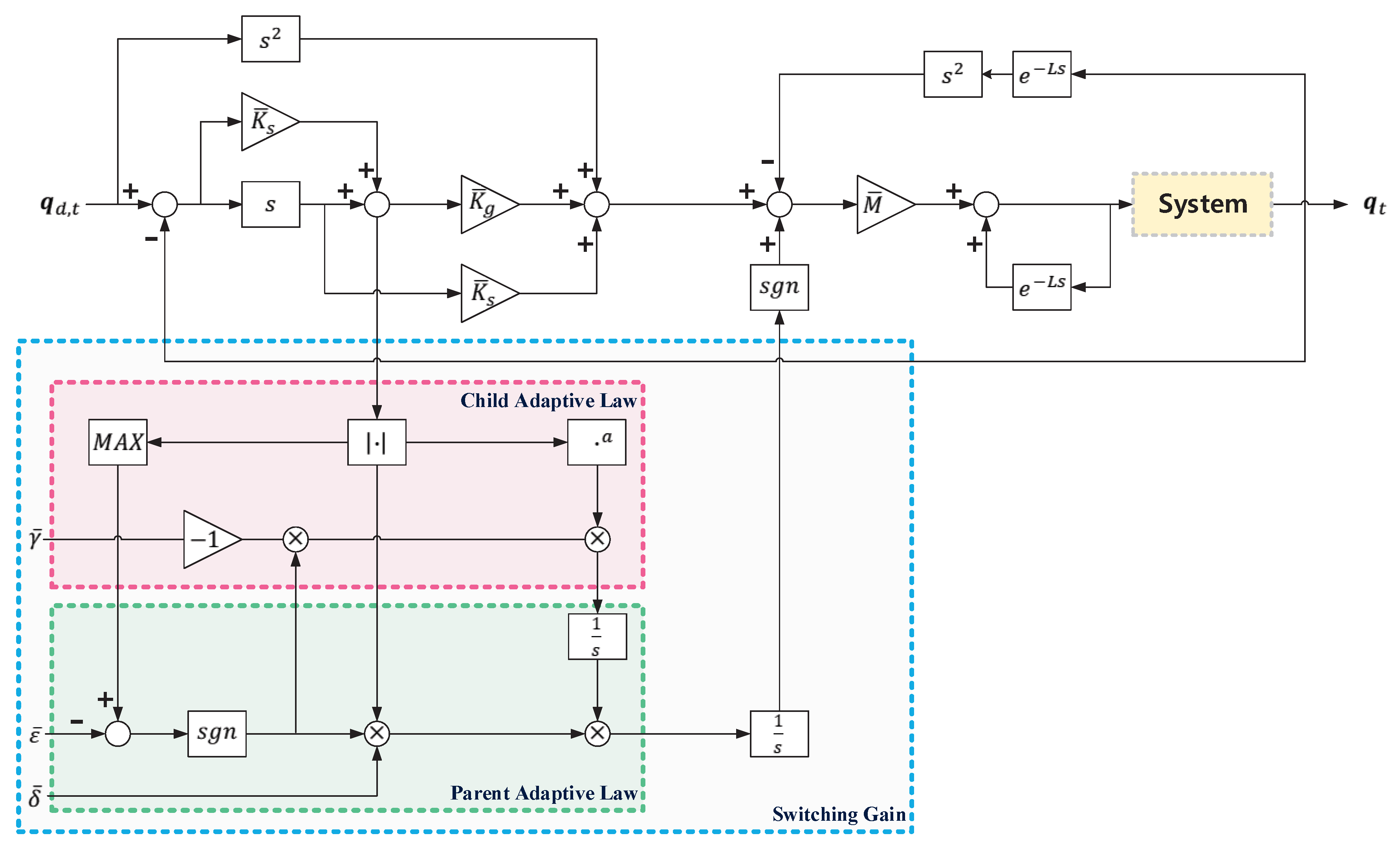
Figure 1. A block diagram of the proposed strong and stable adaptive sliding-mode control (SS-ASMC) approach.
Applsci 10 02909 g001
Figure 2. A 2-link planar robot manipulator.
Applsci 10 02909 g002
Figure 3. Command joint angle trajectories with sinusoidal signal: (a) Joint 1. (b) Joint 2.
Applsci 10 02909 g003
Figure 4. Update parameters generated by the proposed SS-ASMC approach: (a) Joint 1 (× 10 2 ). (b) Joint 2 (× 10 2 ).
Applsci 10 02909 g004
Figure 5. A comparison between the switching gains of the proposed SS-ASMC approach and the existing ASMC approach: (a) Switching gain of the proposed SS-ASMC approach for the Joint 1 (× 10 2 ). (b) Switching gain of the proposed SS-ASMC approach for the Joint 2 (× 10 2 ). (c) Switching gain of the ASMC approach for the Joint 1 (× 10 2 ). (d) Switching gain of the ASMC approach for the Joint 2 (× 10 2 ).
Applsci 10 02909 g005
Figure 6. Sliding variables generated by the proposed SS-ASMC approach: (a) Joint 1. (b) Joint 2.
Applsci 10 02909 g006
Figure 7. Comparison of the tracking errors of time-delayed control (TDC) approach (dotted line), adaptive sliding-mode control (ASMC) approach (dotted dashed line), and the proposed SS-ASMC approach (solid line): (a) Joint 1. (b) Joint 2.
Applsci 10 02909 g007
Table 1. The root-mean-square (RMS) tracking errors for sinusoidal command joint angle trajectory.
Control StrategiesJoint 1 (Deg)Joint 2 (Deg)
TDC approach [32]6.70 × 10 2 40.66 × 10 2
ASMC approach [17]2.92 × 10 2 10.46 × 10 2
Proposed SS-ASMC approach (Equation (12))0.78 × 10 2 4.59 × 10 2