A Supervised Speech Enhancement Approach with Residual Noise Control for Voice Communication

Abstract
:1. Introduction
2. Problem Formulation
3. Proposed Algorithm
3.1. Trade-Off Criterion in Subband
3.2. Trade-Off Criterion in Fullband
3.3. A Generalized Loss Function
4. Experimental Setup
4.1. Dataset
4.2. Experimental Settings
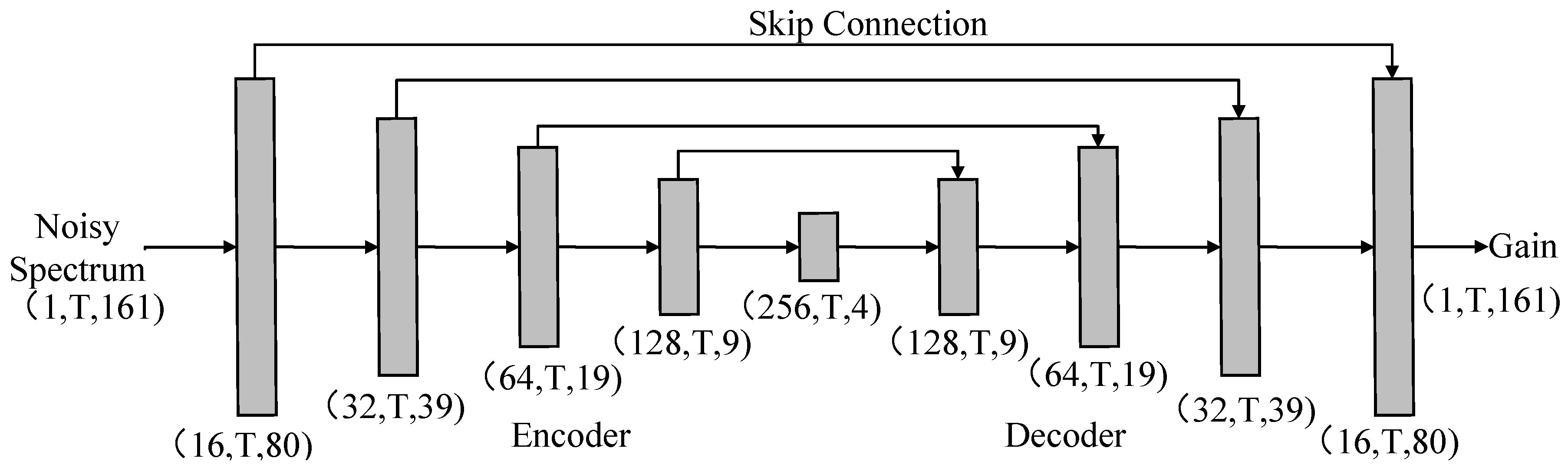
4.3. Network Architecture
4.4. Loss Functions and Training Models
5. Results and Analysis
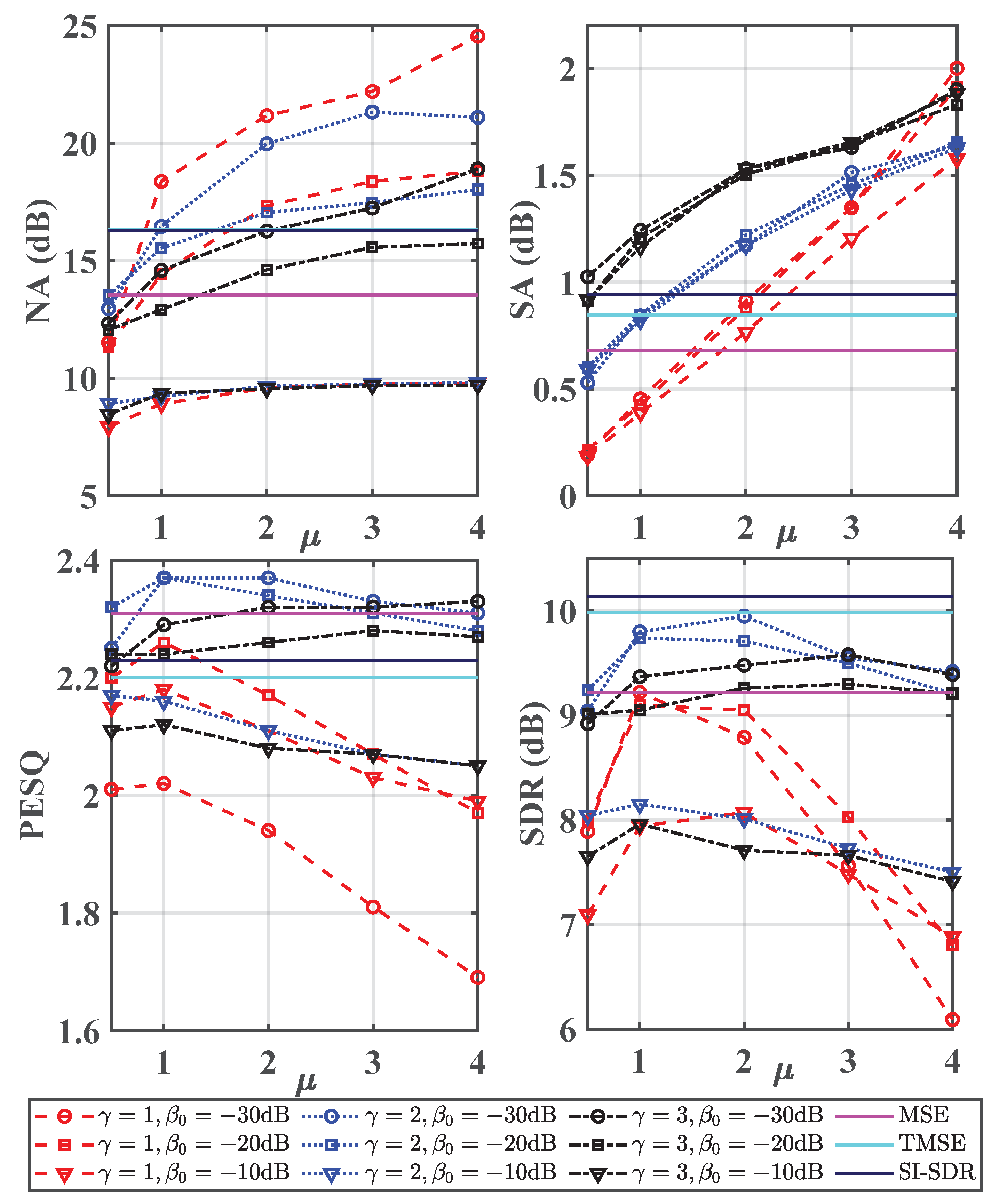
5.1. The Impact of , and
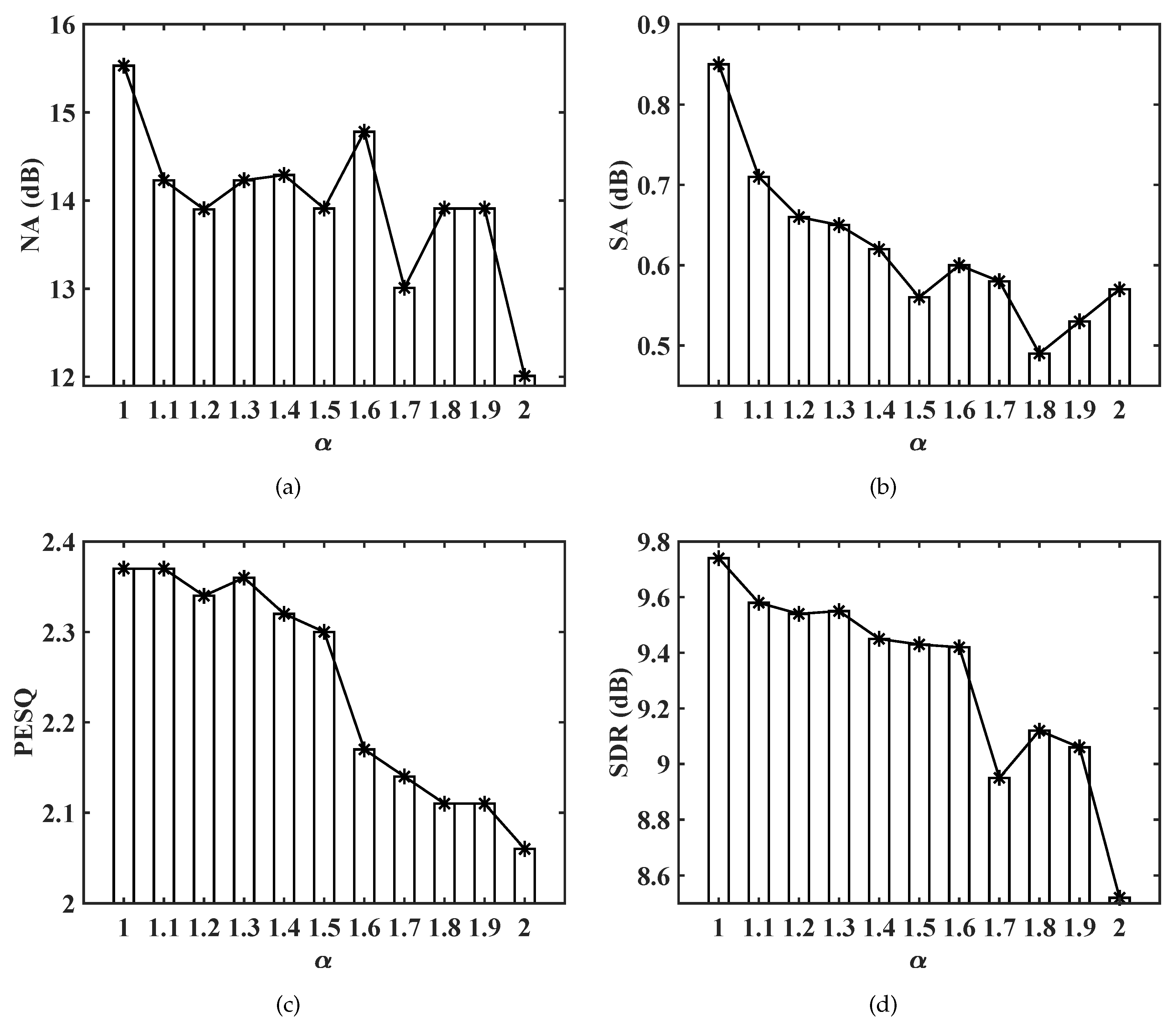
5.2. The Impact of
5.3. Subjective Evaluation
6. Conclusions
Author Contributions
Funding
Conflicts of Interest
Acronyms and Abbreviations
| SNR | signal-to-noise ratio |
| MMSE | minimum mean-squared error |
| MSE | mean-squared error |
| DNN | deep neural network |
| PESQ | perceptual evaluation speech quality |
| STOI | short-time objective intelligibility |
| CL | component loss |
| GL | generalized loss |
| SI-SDR | scale-invariant speech distortion ratio |
| T-F | time-frequency |
| DFT | discrete Fourier transform |
| SGD | stochastic gradient descent |
| STFT | short-time Fourier transform |
| BN | batch normalization |
| ELU | exponential linear unit |
| TMSE | time mean-squared error |
| iSTFT | inverse short-time Fourier transform |
| NA | noise attenuation |
| SA | speech attenuation |
| SDR | speech distortion ratio |
References
- Boll, S. Suppression of acoustic noise in speech using spectral subtraction. IEEE Trans. Acoust. Speech Signal Process. 1979, 27, 113–120. [Google Scholar] [CrossRef] [Green Version]
- Ephraim, Y.; Malah, D. Speech enhancement using a minimum-mean square error short-time spectral amplitude estimator. IEEE Trans. Acoust. Speech Signal Process. 1984, 32, 1109–1121. [Google Scholar] [CrossRef] [Green Version]
- Ephraim, Y.; Malah, D. Speech enhancement using a minimum mean-square error log-spectral amplitude estimator. IEEE Trans. Acoust. Speech Signal Process. 1985, 33, 443–445. [Google Scholar] [CrossRef]
- Ephraim, Y.; Van Trees, H.L. A signal subspace approach for speech enhancement. IEEE Trans. Acoust. Speech Signal Process. 1995, 3, 251–266. [Google Scholar] [CrossRef]
- Wang, Y.; Narayanan, A.; Wang, D. On training targets for supervised speech separation. IEEE Trans. Audio Speech Lang. Process. 2014, 22, 1849–1858. [Google Scholar] [CrossRef] [Green Version]
- Xu, Y.; Du, J.; Dai, L.-R.; Lee, C.-H. An experimental study on speech enhancement based on deep neural networks. IEEE Signal Process. Lett. 2013, 21, 65–68. [Google Scholar] [CrossRef]
- Li, A.; Yuan, M.; Zheng, C.; Li, X. Speech enhancement using progressive learning-based convolutional recurrent neural network. Appl. Acoust. 2020, 166, 107347. [Google Scholar] [CrossRef]
- Zhang, L.; Wang, M.; Zhang, Q.; Liu, M. Environmental Attention-Guided Branchy Neural Network for Speech Enhancement. Appl. Sci. 2020, 10, 1167. [Google Scholar] [CrossRef] [Green Version]
- Wu, J.; Hua, Y.; Yang, S.; Qin, H.; Qin, H. Speech Enhancement Using Generative Adversarial Network by Distilling Knowledge from Statistical Method. Appl. Sci. 2019, 9, 3396. [Google Scholar] [CrossRef] [Green Version]
- Hu, Y.; Loizou, P.C. A perceptually motivated approach for speech enhancement. IEEE Trans. Audio Speech Lang. Process. 2003, 11, 457–465. [Google Scholar] [CrossRef]
- Loizou, P.C.; Kim, G. Reasons why current speech-enhancement algorithms do not improve speech intelligibility and suggested solutions. IEEE Trans. Audio Speech Lang. Process. 2010, 19, 47–56. [Google Scholar] [CrossRef] [Green Version]
- Martín-Doñas, J.M.; Gomez, A.M.; Gonzalez, J.A.; Peinado, A.M. A deep learning loss function based on the perceptual evaluation of the speech quality. IEEE Signal Process. Lett. 2018, 25, 1680–1684. [Google Scholar] [CrossRef]
- Liu, Q.; Wang, W.; Jackson, P.J.; Tang, Y. A perceptually-weighted deep neural network for monaural speech enhancement in various background noise conditions. In Proceedings of the European Signal Processing Conference (EUSIPCO), Kos, Greece, 28 August–2 September 2017; pp. 1270–1274. [Google Scholar]
- Kolbæk, M.; Tan, Z.-H.; Jensen, J. Monaural speech enhancement using deep neural networks by maximizing a short-time objective intelligibility measure. In Proceedings of the IEEE International Conference on Acoustics, Speech, Signal Processing (ICASSP), Calgary, AB, Canada, 15–20 April 2018; pp. 5059–5063. [Google Scholar]
- Venkataramani, S.; Casebeer, J.; Smaragdis, P. Adaptive front-ends for end-to-end source separation. In Proceedings of the Neural Information Processing Systems (NIPS), Long Beach, CA, USA, 4–9 December 2017. [Google Scholar]
- Shivakumar, P.G.; Georgiou, P.G. Perception optimized deep denoising autoencoders for speech enhancement. In Proceedings of the Conference of the International Speech Communication Association (INTERSPEECH), San Francisco, CA, USA, 8–12 September 2016; pp. 3743–3747. [Google Scholar]
- Rim, A.W.; Beerends, J.G.; Hollier, M.P.; Hekstra, A.P. Perceptual evaluation of speech quality (PESQ)-a new method for speech quality assessment of telephone networks and codecs. In Proceedings of the International Conference on Acoustics, Speech and Signal Processing (ICASSP), Salt Lake City, UT, USA, 7–11 May 2001; pp. 749–752. [Google Scholar]
- Taal, C.H.; Hendriks, R.C.; Heusdens, R.; Jensen, J. A short-time objective intelligibility measure for time-frequency weighted noisy speech. In Proceedings of the International Conference on Acoustics, Speech and Signal Processing (ICASSP), Dallas, TX, USA, 15–19 March 2010; pp. 4214–4217. [Google Scholar]
- Le Roux, J.; Wisdom, S.; Erdogan, H.; Hershey, J.R. SDR–half-baked or well done? In Proceedings of the International Conference on Acoustics, Speech and Signal Processing (ICASSP), Brighton, UK, 12–17 May 2019; pp. 626–630.
- Fu, S.; Wang, T.; Tsao, Y.; Lu, X.; Kawai, H. End-to-end waveform utterance enhancement for direct evaluation metrics optimization by fully convolutional neural networks. IEEE Trans. Audio Speech Lang. Process. 2018, 26, 1570–1584. [Google Scholar] [CrossRef] [Green Version]
- Xu, Z.; Elshamy, S.; Zhao, Z.; Fingscheidt, T. Components loss for neural networks in mask-based speech enhancement. arXiv 2019, arXiv:1908.05087. [Google Scholar]
- Zheng, C.; Zhou, Y.; Hu, X.; Li, X. Two-channel post-filtering based on adaptive smoothing and noise properties. In Proceedings of the International Conference on Acoustics, Speech and Signal Processing (ICASSP), Prague, Czech Republic, 22–27 May 2011; pp. 1745–1748. [Google Scholar]
- Zheng, C.; Liu, H.; Peng, R.; Li, X. A statistical analysis of two-channel post-filter estimators in isotropic noise fields. IEEE Trans. Audio Speech Lang. Process. 2012, 21, 336–342. [Google Scholar] [CrossRef]
- Gelderblom, F.B.; Tronstad, T.V.; Viggen, E.M. Subjective evaluation of a noise-reduced training target for deep neural network-based speech enhancement. IEEE/ACM Trans. Audio Speech Lang. Process. 2018, 27, 583–594. [Google Scholar] [CrossRef]
- Gustafsson, S.; Jax, P.; Vary, P. A novel psychoacoustically motivated audio enhancement algorithm preserving background noise characteristics. In Proceedings of the International Conference on Acoustics, Speech and Signal Processing (ICASSP), Seattle, WA, USA, 12–15 May 1998; pp. 397–400. [Google Scholar]
- Braun, S.; Kowalczyk, K.; Habets, E.A. Residual noise control using a parametric multichannel wiener filter. In Proceedings of the International Conference on Acoustics, Speech and Signal Processing (ICASSP), New Orleans, LA, USA, 5–9 March 2015; pp. 360–364. [Google Scholar]
- Benesty, J.; Chen, J.; Huang, Y.; Cohen, I. Noise Reduction in Speech Processing; Springer: Berlin/Heidelberg, Germany, 2009. [Google Scholar]
- Martin, R. Noise power spectral density estimation based on optimal smoothing and minimum statistics. IEEE Trans. Speech Audio Process. 2001, 9, 504–512. [Google Scholar] [CrossRef] [Green Version]
- Cohen, I. Noise spectrum estimation in adverse environments: Improved minima controlled recursive averaging. IEEE Trans. Speech Audio Process. 2003, 11, 466–475. [Google Scholar] [CrossRef] [Green Version]
- Gerkmann, T.; Hendriks, R.C. Unbiased mmse-based noise power estimation with low complexity and low tracking delay. IEEE Trans. Audio Speech Lang. Process. 2011, 20, 1383–1393. [Google Scholar] [CrossRef]
- Inoue, T.; Saruwatari, H.; Shikano, K.; Kondo, K. Theoretical analysis of musical noise in wiener filtering family via higher-order statistics. In Proceedings of the International Conference on Acoustics, Speech and Signal Processing (ICASSP), Prague, Czech Republic, 22–27 May 2011; pp. 5076–5079. [Google Scholar]
- Duan, Z.; Mysore, G.J.; Smaragdis, P. Speech enhancement by online non-negative spectrogram decomposition in nonstationary noise environments. In Proceedings of the Conference of the International Speech Communication Association (INTERSPEECH), Portland, OR, USA, 9–13 September 2012; pp. 1–4. [Google Scholar]
- Varga, A.; Steeneken, H.J. Assessment for automatic speech recognition: Ii. noisex-92: A database and an experiment to study the effect of additive noise on speech recognition systems. Speech Commun. 1993, 12, 247–251. [Google Scholar] [CrossRef]
- Kingma, D.P.; Ba, J. Adam: A method for stochastic optimization. arXiv 2014, arXiv:1412.6980. [Google Scholar]
- Kolbæk, M.; Tan, Z.-H.; Jensen, S.H.; Jensen, J. On loss functions for supervised monaural time-domain speech enhancement. arXiv 2019, arXiv:1909.01019. [Google Scholar] [CrossRef] [Green Version]
- Ioffe, S.; Szegedy, C. Batch normalization: Accelerating deep network training by reducing internal covariate shift. In Proceedings of the International Conference on Machine Learning (ICML), Lille, France, 6–11 July 2015; pp. 448–456. [Google Scholar]
- Clevert, D.-A.; Unterthiner, T.; Hochreiter, S. Fast and accurate deep network learning by exponential linear units (elus). arXiv 2015, arXiv:1511.07289. [Google Scholar]
- Wichern, G.; Roux, J.L. Phase reconstruction with learned time-frequency representations for single-channel speech separation. In Proceedings of the International Workshop on Acoustic Signal Enhancement (IWAENC), Tokyo, Japan, 17–20 September 2018; pp. 396–400. [Google Scholar]
- Vincent, E.; Gribonval, R.; Févotte, C. Performance measurement in blind audio source separation. IEEE/ACM Trans. Audio Speech Lang. Process. 2006, 14, 1462–1469. [Google Scholar] [CrossRef] [Green Version]
- Breithaupt, C.; Gerkmann, T.; Martin, R. Cepstral smoothing of spectral filter gains for speech enhancement without musical noise. IEEE Signal Process. Lett. 2007, 14, 1036–1039. [Google Scholar] [CrossRef]


| Layer Name | Input Size | Hyperparameters | Output Size |
|---|---|---|---|
| reshape_size_1 | T × 161 | - | 1 × T × 161 |
| conv2d_1 | 1 × T × 161 | 2 × 3, (1, 2), 16 | 16 × T × 80 |
| conv2d_2 | 16 × T × 80 | 2 × 3, (1, 2), 32 | 32 × T × 39 |
| conv2d_3 | 32 × T × 39 | 2 × 3, (1, 2), 64 | 64 × T × 19 |
| conv2d_4 | 64 × T × 19 | 2 × 3, (1, 2), 128 | 128 × T × 9 |
| conv2d_5 | 128 × T × 9 | 2 × 3, (1, 2), 256 | 256 × T × 4 |
| deconv2d_1 | 256 × T × 4 | 2 × 3, (1, 2), 128 | 128 × T × 9 |
| skip_1 | 128 × T × 9 | - | 256 × T × 9 |
| deconv2d_2 | 256 × T × 9 | 2 × 3, (1, 2), 64 | 64 × T × 19 |
| skip_2 | 64 × T × 19 | - | 128 × T × 19 |
| deconv2d_3 | 128 × T × 19 | 2 × 3, (1, 2), 32 | 32 × T × 39 |
| skip_3 | 32 × T × 39 | - | 64 × T × 39 |
| deconv2d_4 | 64 × T × 39 | 2 × 3, (1, 2), 16 | 16 × T × 80 |
| skip_4 | 16 × T × 80 | - | 32 × T × 80 |
| deconv2d_5 | 32 × T × 80 | 2 × 3,(1, 2), 1 | 1 × T × 161 |
| reshape_size_2 | 1 × T × 161 | - | T × 161 |
| Methods | GL | MSE | Equal |
|---|---|---|---|
| Preference | 70.0% | 22.0% | 8.0% |
| Methods | GL | TMSE | Equal |
| Preference | 66.5% | 22.0% | 12.5% |
| Methods | GL | SI-SDR | Equal |
| Preference | 70.5% | 23.5% | 6.0% |
© 2020 by the authors. Licensee MDPI, Basel, Switzerland. This article is an open access article distributed under the terms and conditions of the Creative Commons Attribution (CC BY) license (http://creativecommons.org/licenses/by/4.0/).
Share and Cite
Li, A.; Peng, R.; Zheng, C.; Li, X. A Supervised Speech Enhancement Approach with Residual Noise Control for Voice Communication. Appl. Sci. 2020, 10, 2894. https://doi.org/10.3390/app10082894
Li A, Peng R, Zheng C, Li X. A Supervised Speech Enhancement Approach with Residual Noise Control for Voice Communication. Applied Sciences. 2020; 10(8):2894. https://doi.org/10.3390/app10082894
Chicago/Turabian StyleLi, Andong, Renhua Peng, Chengshi Zheng, and Xiaodong Li. 2020. "A Supervised Speech Enhancement Approach with Residual Noise Control for Voice Communication" Applied Sciences 10, no. 8: 2894. https://doi.org/10.3390/app10082894
APA StyleLi, A., Peng, R., Zheng, C., & Li, X. (2020). A Supervised Speech Enhancement Approach with Residual Noise Control for Voice Communication. Applied Sciences, 10(8), 2894. https://doi.org/10.3390/app10082894