Abstract
Real-time positron emission tomography (PET) may provide information from first-shot images, enable PET-guided biopsies, and allow awake animal studies. Fully-3D iterative reconstructions yield the best images in PET, but they are too slow for real-time imaging. Analytical methods such as Fourier back projection (FBP) are very fast, but yield images of poor quality with artifacts due to noise or data incompleteness. In this work, an image reconstruction based on the pseudoinverse of the system response matrix (SRM) is presented. w. To implement the pseudoinverse method, the reconstruction problem is separated into two stages. First, the axial part of the SRM is pseudo-inverted (PINV) to rebin the 3D data into 2D datasets. Then, the resulting 2D slices can be reconstructed with analytical methods or by applying the pseudoinverse algorithm again. The proposed two-step PINV reconstruction yielded good-quality images at a rate of several frames per second, compatible with real time applications. Furthermore, extremely fast direct PINV reconstruction of projections of the 3D image collapsed along specific directions can be implemented.
1. Introduction
1.1. Motivation
Positron emission tomography (PET) is widely used in medical imaging. In many applications of PET such as first-shot tests for chemicals [1] or PET image-guided surgery or biopsy [2], it is crucial to obtain images as quickly as possible. The frame rate achievable will depend on the sensitivity of the acquisition system, the hardware used for data acquisition, and the software employed for data processing and image reconstruction [3]. State-of-the-art PET systems [4,5,6] can process up to 10 million coincidences per second, providing useful images in very short time frames. The challenge to be considered here is to provide useful quasi real-time images, that is, at a rate of a few frames per second with appropriate image quality.
Tomographic PET image reconstruction methods are usually classified into analytical [7,8], and iterative methods [9,10,11]. In order to be applicable, analytical methods such as filtered back projection (FBP) require many assumptions such as ideal detection, uniform sampling, data completeness, and noise properties to build the system response matrix (SRM) [12]. Although these assumptions are quite reasonable for computed tomography (CT) imaging [13], they are questionable in PET, making these reconstructions of suboptimal quality [10,14,15,16]. Another disadvantage of analytical methods is that the resolution of the images is not uniform across the field of view (FOV), which affects quantification [17]. On other hand, iterative reconstructions provide better results than analytical methods [9,18], thanks to the incorporation in the reconstruction process of the physics effects involved in the emission, transport, and detection of PET radiation [14] such as positron range [19], non-collinearity, depth-of-interaction (DOI) in the crystals [13], geometrical considerations of the scanner [18,20], etc. However, iterative methods with realistic SRM are slow, and therefore, their application to real-time fully 3D PET imaging is still challenging [3,7].
One of the most common approaches to speeding-up the reconstruction process involves introducing axial rebinning of the data, followed by 2D reconstructions [7,21,22]. The simplest method for axial rebinning of PET data is single-slice rebinning (SSRB) [23], where the activity is assigned to the central axial coordinate z of both crystals z1, z2. This method is very fast, however, it is only accurate for activity close to the axis of the scanner. A more accurate alternative to SSRB is Fourier rebinning (FORE) [24], but unfortunately, it is much slower.
Here, we propose the pseudoinverse (PINV) of the SRM [25] to achieve real-time reconstructions with uniform resolution [26]. The goal was to achieve some of the features of iterative methods with the computational cost of analytical reconstructions, thus providing fast reconstructions while incorporating the physics involved [18].
1.2. Theory
1.2.1. Separation of the System Response Matrix (SRM) into Axial and Transaxial Components
The line-of-response (LOR) of a given coincidence event is defined as the line connecting the crystals where the detection took place [27]. These LORs are usually organized in 3D-sinograms with coordinates (ρ,θ,z1,z2) (see Figure 1). Note that the axial position of the LOR (z) and its axial slope angle (Δ) are usually used instead of z1, z2 [9,28,29]. For convenience and for easier explanation, in this work, we use the notation z1, z2.
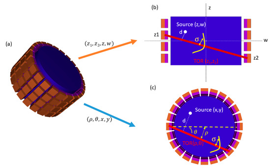
Figure 1.
(a) 3D Positron emission tomography (PET) scanner and computation of system response matrices (SRMs). (b) Axial SRM. A source placed in position in the rebinned data space, can produce a coincidence in a tube of response (TOR) of width σ. The probability depends on the distance d from the source to the line of response (LOR). (c) Transaxial SRM. A source placed in position (x,y) in the field of view can produce a coincidence in a TOR of width . The probability depends on the LOR–source d.
The SRM contains the probability that a decay at a position (x, y, z) in the image space is detected in a specific LOR with coordinates (ρ,θ,z1,z2) in the projection space [9,14,30,31]. The SRM in 3D acquisitions is usually too large (of the order of terabytes) to be kept in the memory of current computers. In most iterative methods, these huge matrices are handled with sparse methods [32] or the storage requirement is reduced by exploiting symmetries [9]. However, the computation of the PINV of the SRM does require the use of the whole matrix, because even when the SRM is sparse, the pseudoinverse may not be [33,34]. To solve this issue, we decomposed the SRM into axial Az and transaxial Ax,y components:
Ax,y,z (ρ,θ,z1,z2,x,y,z) ≅ [Ax,y (ρ,θ,x,y);Az (z1,z2,z)],
The axial matrix can be used for data rebinning and the transaxial matrix for 2D reconstruction of the rebinned 2D slices.
1.2.2. Computation of the SRM
SRMs can be obtained from Monte Carlo simulations [9,20,31] approximated by analytical expressions [35] (Reader 2003), or even measured experimentally [36]. In this work, we used analytic SRMs. To model the problem more realistically for each LOR, we defined a tube of response (TORs) [37], where its width reflects the physical effects. In this work, TORs were assumed to have a Gaussian cross section [18,38,39], whose width () was obtained empirically for a given scanner, being the same for all LORs of the same scanner.
To derive the axial SRM, we considered an image space discretized in axial (z) and length coordinates (w) along the LOR (Figure 1b). The probability for each voxel to be connected to a given LOR was obtained as follows:
where is the minimum distance between the voxel at and the LOR given by (Figure 1b).
In a similar way, each element of the transaxial SRM can be modeled as (Figure 1c):
where is the distance from the voxel to the LOR [39].
In order to ease operations with these matrices, we combined some variables in the same bin index. We used and instead of and . In what follows, we will use this notation.
1.2.3. Pseudoinverse of the SRM
The solution of the least-squares problem [40] for a system with linear equations () can be obtained using the pseudoinverse of the matrix [41,42,43]:
The singular value decomposition (SVD) [44,45,46,47,48] was used here to compute the pseudoinverse of the matrix. In this method, matrix is first decomposed into the product of two orthonormal matrices and and a diagonal matrix containing the singular values () of :
With that decomposition, the pseudoinverse of the matrix results:
where the reciprocal singular values of the matrix are given by .
1.2.4. Regularization of the Pseudoinverse
As can be noted, when singular values are very small or null, their reciprocals are not well defined. Small singular values correspond to high frequency elements, which contain the finer details of the image (interesting to keep) as well as most of the noise of the data [15,16,49] (which amplifies the noise in the reconstructed image). To deal with this problem, we used regularization methods [50]. A common regularization approach is truncated singular value decomposition (TSVD), which is obtained by setting to the reciprocal singular values larger than a chosen threshold [51].
A less extreme approach is Tikhonov regularization [50], which replaces the reciprocal singular values 1/s by:
where k is a regularization parameter [52,53].
Very often in iterative reconstruction methods, the number of iterations serves as a regularization parameter [54]. A small number of iterations corresponds to large regularizations. In fact, it was found that a PINV regularization scheme such as the resulting images coincided with the ones of the iterative Landweber algorithm [55]. The Landweber regularization would replace the reciprocal values by (see Appendix A) [56]:
where n is the number of Landweber iterations. This implies that through the PINV, an iterative Landweber reconstruction can be performed in one single step.
Furthermore, the number of iterations in a Landweber regularization (Figure 2) can be related with the regularization parameter k in Tikhonov regularization as:
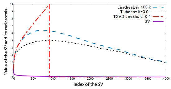
Figure 2.
Singular values of a small matrix (solid line) and its reciprocals using different regularization methods. Tikhonov (k = 0.01) and Landweber (n = 100) regularization for equivalent iterations. Truncated singular values (TSVD) with a threshold of 0.1 and original singular values (SV) are also shown.
We present our results in terms of equivalent Landweber iterations, allowing us to study resolution recovery and noise in the image in terms of the number of equivalent iterations, as is usually done for iterative methods.
1.2.5. Axial Rebinning and Transaxial Reconstruction with the Pseudoinverse
Following the way the SRM was modeled into two independent components, the reconstruction process can be split into two smaller problems: axial rebinning (PINVz) and 2D reconstruction of the corresponding rebinned slices (2D-PINV).
was obtained as the pseudoinverse of obtained from Equation (2) and then collapsing (summing over) in t. On the other hand,
where is the pseudoinverse of , obtained from Equation (3).
Since both processes are independent and only involve matrix products, the reconstruction can be performed in a single step in which the 3D data are multiplied by each matrix from the left and right:
The workflow of the reconstruction process is represented schematically in Figure 3.

Figure 3.
Workflow of the reconstruction process. 3D data are multiplied PINVs of the axial and transaxial SRMs in a single step.
1.2.6. List-Mode Data and Event by Event Reconstruction
As it has been shown in previous works [3], the pseudoinverse of the SRM can be used for list-mode data reconstruction. In a 3D problem, each column of the PINV of the SRM, , contains the region of the image that would produce a coincidence in the given LOR . Taking this into account, the image can be refreshed after every event. A similar approach is also feasible in the proposed scheme. Each coincidence with coordinates can be separated into transaxial and axial coordinates. Using , for every coincidence with axial coordinates, each z slice of the image is weighted by the corresponding element of the pseudoinverse of the axial SRM . Then, for each axial slice, coordinates of the image are updated event by event using each row of the transaxial SRM pseudoinverse . Although this is fast and feasible for a 2D case as presented by Selivanov and Lecompte [3], it takes longer than reconstructing with the whole sinogram, except for when the number of coincidences is very small. In our case, reading the list-mode coincidences and histograming them in a sonogram is faster than event by event reconstruction, even for frames as small as 0.1 s for the preclinical SuperArgus PET-CT scanner introduced in Section 2.2.1.
1.2.7. Projection over Planes
In many cases, real-time images are used to follow radiotracer distribution along the body of a patient for which the sum of the image collapsed in specific directions instead of a 3D presentation of the full image may be enough. This way of presenting real-time PET images is also convenient as short frame images would typically contain a very low number of counts, and 2D projections will be less noisy in this case.
In general, to obtain images collapsed over planes, a 3D image is needed, which is later projected. However, using the pseudoinverse, this process can be reduced to one single step, if the pseudoinverse, instead of the image, is collapsed once and for all. This leads to much smaller PINV matrices, and thus much faster matrix products.
In this work, we used 2D-PINV matrices collapsed over the X and Y directions. These matrices, combined with PINVz, produces projections in the XZ and YZ planes, respectively. Note that if we sum over all the slices obtained from the rebinning step, and then reconstruct the resulting slice, we obtain the equivalent of the 3D image collapsed into the XY plane.
2. Materials and Methods
2.1. Simulated Data
PeneloPET [57] was used for the simulations presented in this work. It is a Monte-Carlo simulator, based on PENELOPE [58]. It considers the main physical effects during PET acquisitions such as positron range [19], non-collinearity, nuclear decay of the isotope, etc.
18F point sources (radius 0.5 mm) were simulated for a geometry similar to the Biograph TPTV (Siemens) scanner [58] to evaluate the axial resolution of the different rebinning strategies discussed. The image noise was evaluated with another simulation of two homogeneous cylinders. The axial resolution was obtained from the full width at half maximum (FWHM) of the 1D-Gaussian fit to the axial profile obtained in the center of each source. The noise level was obtained as the ratio of the standard deviation to the average value in spherical Regions Of Interest (ROI’s) with a radius of 5 cm located inside the simulated cylinders.
We used the same sinogram dimensions as the actual clinical scanner data described below. The rebinned 2D slices were reconstructed using FBP with a Hamming filter (cutoff 0.5).
A thin slice Defrise phantom [59] was simulated to study axial rebinning with different methods. In this case, the simulated geometry was the one corresponding to the preclinical SuperArgus PET-CT scanner (SEDECAL) [6]. The simulated phantom was composed of several disks of 8 cm diameter and 3 mm thickness. The gap between disks was 3 mm. We used the same sinogram dimensions as the actual preclinical scanner data, as described in Section 2.2.1.
2.2. Real Data
2.2.1. Preclinical PET/CT Scanner
We used the six ring version of the SuperArgus PET/CT scanner (Figure 4. (left)). This configuration consists of 24 arrays of 13 13 crystals with 1.55 mm pitch size. The number of sinogram bins was 175 (radial) 128 (angular). Radial bins were 0.5 mm in size, configuring a 8.75 cm transaxial FOV. A total of 195 slices of 0.775 mm each were used in the axial direction. The maximum ring difference [28] was set to 97 and a span factor of 19 was applied, resulting in a total of 1185 sinograms. The axial pseudoinverse matrices had a size of 1185 × 195. For the 2D matrices, 175 voxels were chosen for the image FOV. The size of 2D matrices for the SuperArgus PET/CT was around 2.6 Gb. Both of the Gaussian distributions of the TOR were 0.6 mm.
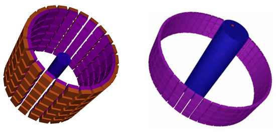
Figure 4.
Schematic representation of the SuperArgus (left) and the Biograph TPTV scanners (right) simulated in PeneloPET.
For the evaluation of the image quality we used the IQ NEMA and Derenzo phantoms [60]. The rod diameters (Derenzo phantom) were 1.2, 1.6, 2.4, 3.2, 4, and 4.8 mm.
Two animal acquisitions injected with fluorodeoxyglucose (FDG) were also used to evaluate the performance of the PINV (PINVz + 2D-PINV) methodology: a 200 g rat and a cardiac acquisition of a 15 g mouse. Over the cardiac mouse acquisition, a quantitative comparison of 2D-PINV and FBP in real preclinical acquisitions was made. A profile over the heart was fit to two Gaussians (one to each side of the heart). The average of the standard deviation of both Gaussians is shown and the relative improvement of 2D-PINV over FBP was calculated as . Moreover, we used a first pass acquisition of a mouse injected with FDG to demonstrate the real-time capabilities of PINV reconstructions.
Acquisitions were performed at the Instituto de Investigación Sanitaria Gregorio Marañón (Madrid, Spain). All experimental procedures were done in compliance with the European Communities Council Directive 2010/63/EU and submitted for approval to the Institutional Animal Care and Use and Ethics Committee of the Hospital General Universitario Gregorio Marañón (HGUGM), supervised by the Comunidad de Madrid, according to the Annex X of the RD 53/2013. The subjects were kept at the animal housing facilities of the Unidad de Medicina y Cirugía Experimental (UMCE-HGUGM) in Madrid, Spain.
2.2.2. Clinical PET/CT Scanner
For the clinical data, we used 18F acquisitions obtained with a Biograph TPTV [58,61] (Figure 4. (right)) scanner at the Medical University of Vienna (Austria) with a 34 cm radial field of view, four rings of 48 arrays with 13 13 scintillator crystals, with an axial length of 4 mm of each crystal. The total number of radial and angular sinogram bins was 336 336 [61]. Radial bins were 2.024 mm in size. A total of 109 slices of 2 mm each were used in the axial direction. The maximum ring difference was set to 38 and a span factor of 11 was applied, yielded into 559 sinograms. The axial matrices had a size of 559 109 (238 KB). For the 2D matrices, 225 voxels were chosen, providing a FOV of 45.54 cm. The size of the 2D matrices was around 21 GB. The and for the TORs in the matrices were 2 mm.
2.3. Image Quality Evaluation
We evaluated the reconstructed images of the phantoms following the National Electrical Manufacturers Association (NEMA) NU 2-2007 and NU 4-2008 protocols for clinical and preclinical phantoms, respectively [62,63].
- Noise level in the image (%): evaluated as the standard deviation of the activity in a uniform region divided by the average activity in that region.
- Resolution (%), following the NEMA standards [62,63].
For the preclinical scanner, the mouse-size IQ phantom was used.
Sinograms were corrected by attenuation and random coincidences. In the case of the clinical NEMA, scatter corrections were also included.
We present a comparison of SSRB + FBP or FORE + FBP with the proposed method (PINVz + 2D-PINV). Unless otherwise noted, execution times correspond to one thread of a CPU E5-2640 v4 @ 2.40 GHz in a Linux computer with Centos 7 OS.
3. Results
3.1. Simulated Data and Axial Rebinning
Figure 5 shows resolution recovery and noise of four point sources located at different radial and axial positions. Off-axis sources in SSRB reconstructions exhibit much worse resolution than the other two rebinning methods studied. FORE provided the best axial resolution and less noise, while PINV, on the other hand, provided a more uniform resolution and noise level across the FOV, clearly improving SSRB for off-axis values, where it approached the best results of FORE. Indeed, with a proper regularization parameter (around the equivalent to 8 Landweber iterations), similar results in terms of resolution and noise were obtained for the sources placed at 10 cm radially from the center of the scanner using PINV and FORE.
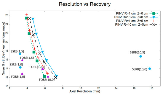
Figure 5.
Noise vs. resolution recovery for different rebinning methods (SSRB, FORE, and PINVz). Point sources were simulated in a scanner with a geometry similar to Biograph TPTV with MRD 38 and SPAN 11. Numbers in brackets at the FORE and SSRB points indicate the distance (R,Z) to the center of the scanner in cm, for example, (10,0) represents a source at a radial distance of 10 cm from the center of the scanner at the axis. Several points for PINVz show the axial resolution vs. recovery for a different Landweber iterations, from right to left 5, 8, 10, 15, and 20 iterations. Outside the axis of the scanner, SSRB was not accurate, while FORE provided the best results overall, although with some sensitivity to distance to the scanner axis. PINVz keeps a more uniform resolution across the whole FOV.
In Figure 6, we can see a coronal view of the reconstruction of a Defrise disk phantom where an improvement in the pseudoinverse rebinning can be appreciated when compared to SSRB. We can see that FORE and PINVz also provided similar detail.
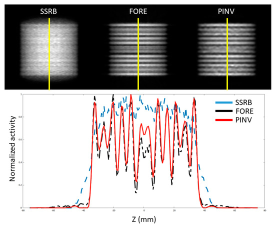
Figure 6.
Axial profile of a simulated thin-slice (XX mm slices thickness) Defrise phantom for the SuperArgus scanner reconstructed from the three rebinning methods (top) and a profile along the axis of the scanner (bottom), that is, along the yellow line in the top panel. PINVz rebinning employed 20 iterations.
3.2. Preclinical Data
Results of a PINV reconstruction (PINVz + 2D-PINV) were compared with the FORE + FBP images. We also studied the isolated 2D reconstruction with FBP and PINV from the same FORE rebinned sinogram for the IQ-NEMA phantom. These results are presented in Figure 7 and Table 1.
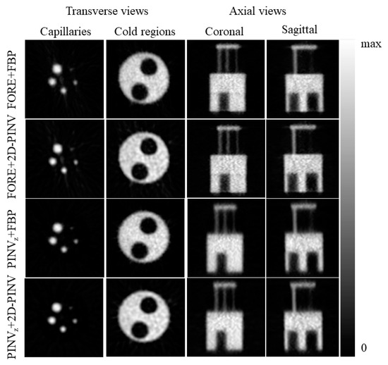
Figure 7.
Fourier Rebinning (FORE) and axial Pseudoinverse (PINVz) rebinned data, coupled with different 2D reconstruction (Filtered Back-Projection (FBP) and 2D Pseudoinverse (2D-PINV)) for the Image Quality National Electrical Manufacturers Association (IQ NEMA) phantom.

Table 1.
Recovery coefficients and uniformity according to NEMA 4-2008.
In Table 1, we compared the recovery coefficients for the IQ-NEMA phantom at approximately the same level of uniformity for every rebinning + 2D reconstruction combination. The 2D-PINV slice reconstruction systematically outperformed (around 5–10% better for the smallest capillary and up to 15% in the 2 mm capillary). As expected, FORE rebinning provided the best recovery, improving marginally on the pseudoinverse rebinning results.
Furthermore, in Figure 8, we present the results for a Derenzo filled with 250 μCi of 18FDG measured with a well-counter with an accuracy of ±5% [11]. It can be seen as an improvement in resolution for 2D-PINV reconstruction when compared to FBP.

Figure 8.
Five centimeter diameter Derenzo phantom. Rods were 1.2, 1.6, 2.4 3.2, 4, and 4.8 mm in diameter. (Left) Reconstructed with 2D-PINV and FBP, respectively, from same sinogram rebinned with FORE. We show the 10 axial slices summed up. (Right) Profile along the yellow line showing the 1.6 and 3.2 mm rods.
Figure 9 shows the cardiac region of a 15 g mouse injected with 170 μCi of 18FDG, with slices reconstructed with FBP and 2D-PINV from a PINV rebinned sinogram. Improvement in spatial resolution (a relative 15%) for 2D-PINV reconstructions can be clearly seen.
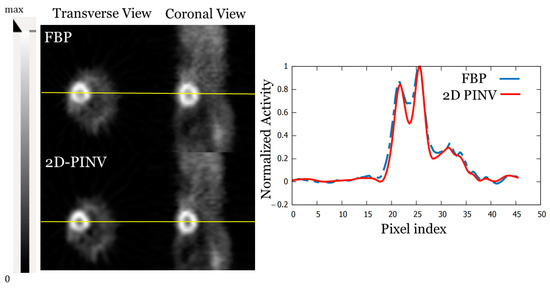
Figure 9.
FBP and 2D-PINV reconstruction of a 15 g mouse injected with 170 μCi of 18FDG from data rebinned using PINV. A profile along the heart is also shown.
Figure 10 shows the PINVz + 2D-PINV versus SSRB + FBP reconstructions of a 200 g rat injected with 300 μCi of 18FDG where the improvement using PINV was evident. Images from both 30 min (bottom) and 5 s (top) acquisitions are shown, the second demonstrating the capabilities for near real time imaging.
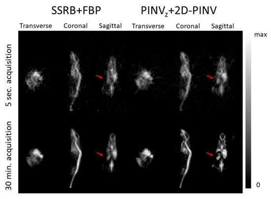
Figure 10.
(Left) SSRB + FBP and (right) PINVz + 2D-PINV image reconstruction of a rat injected with 300 μCi 18FDG. The transverse, coronal and sagittal views are shown for a slice of the image. Top (bottom) panel shows 5 s (1800 s) acquisition.
3.3. Clinical Scanner
We studied the recovery coefficients for the clinical IQ NEMA phantom from images rebinned with SSRB, FORE, and PINVz and reconstructed with the same parameters as in Section 3.1 (i.e., FBP with a Hamming filter). Additionally, we studied a reconstruction PINVz + 2D-PINV. Table 2 shows the recovery coefficients and uniformity over the six spheres following NEMA 2-2007. These results are summarized in Figure 11 and Table 2.

Table 2.
Recovery Coefficients (RC) and noise for the clinical IQ NEMA phantom (NEMA NU 2-2017).

Figure 11.
Transverse FBP and 2D-PINV images from data rebinned with PINV, FORE, and SSRB for the clinical IQ NEMA phantom.
3.4. Reconstruction Time
Reconstruction times are shown in Table 3 and Table 4. Time to generate the pseudoinverse matrix from the SRM and pre-load it to RAM memory was not included as part of the reconstruction, as both processes are performed before it.

Table 3.
Central Processing Unit (CPU) time for the different rebinning methods using a single core of an Intel E5-2640 v4 @ 2.40 GHz processor, with CENTOS 7 Linux OS.

Table 4.
Central Processing Unit (CPU) time for the different 2D reconstruction methods using a single core of an Intel E5-2640 v4 @ 2.40 GHz processor with CENTOS 7 Linux OS.
3.5. Real-Time PET Image Reconstruction
As described in the previous sections, pseudoinverse methods allow for extremely fast, direct reconstruction of projected or collapsed images into any plane. Figure 12 shows the results of a reconstruction collapsed onto the YZ plane during a first shot acquisition for a 13 g mouse injected with 120 μCi of 18FDG, on the SuperArgus scanner. Six frames of one second each are presented, clearly showing the activity coming in along the tail vein and further into the lungs, vascularity, and remaining circulatory system. The reconstruction of the accumulated 6 s is also shown for reference.

Figure 12.
YZ plane reconstructed with PINVz + 2D-PINV of a 13 g mouse injected with 120 μCi of 18FDG.
Table 5 presents the total time needed to obtain these reconstructions using a multithreaded version of the code.

Table 5.
Total (wall clock) time required for direct reconstruction of direct 2D projections using the 2D PINV + PINVz code with eight threads of an Intel E5-2640 v4 @ 2.40 GHz processor (multithreaded enabled, up to 20 threads out of 10 physical cores in this processor). Data were arranged into 175 x 128 x 1185 sinograms.
4. Discussion
In this work, we showed that pseudoinverse reconstruction of 3D PET data using PINVz + 2D-PINV provided better (Table 1 and Table 2) and faster reconstructions than SSRB + FBP (Table 3 and Table 4). It is worth noting that in FBP, it is further needed to estimate the missing data (filling in the gaps in between detectors) [22], and this time was left out from Table 4. On the other hand, pseudoinverse reconstruction only requires knowing the position of the missing data in order to skip those, further speeding the process. Pseudoinverse axial rebinning was much faster than FORE, with just a moderately worse performance in terms of noise/resolution. As has been noted in previous works [3], there is a 2D-PINV matrix that would be fully equivalent to FBP. However, in the construction of the 2D-PINV, it is also possible to add geometrical information and physics effects, which introduce blurring to the TORs. This is the main reason for the improved resolution of in-slice PINV images compared to FBP ones. The matrices for PINV rebinning and slice reconstruction can be precomputed and stored once and for all for a given scanner, making it easy for the user to produce their own reconstructions.
Although it would be desirable to apply PINV methods in 3D altogether instead of the division into axial and transaxial components employed in this work, building a 3D PINV matrix currently seems impractical as 3D PINV arrays for modern complex scanners will not fit in the memory of common computers. Furthermore, as we have presented here, the noise exhibited by PINV rebinning methods is slightly larger than that of FORE. Better regularization techniques [50] or improvements in the SRM could remedy this.
New regularization techniques could involve filtering of the reconstructed image or even the data before reconstruction. Any linear filter (F) can be applied during PINV reconstruction from its matrix representation:
Therefore, applying the filter in the pseudoinverse before the reconstruction would result in the same image as using the filter over the reconstructed image. The same applies to any linear filter applied in the data domain:
Matrices to represent the SRM in this work were obtained analytically for convenience, but they can also be obtained from Monte Carlo simulations, with likely improvement in image quality without affecting the speed of the method.
Reconstruction times presented in Section 3.4 corresponded to only one CPU core. Multi-CPU or Graphics Processing Unit (GPU) strategies can be used to further accelerate the reconstructions. For instance, we have verified a very straightforward method to use multicore 2D by assigning each slice to a CPU-thread, reducing the total time almost linearly within the number of threads employed. In Table 3 and Table 4, reconstruction times for smaller sinograms were also presented. Although some resolution was lost with these smaller sinograms, their very short reconstruction times make them suitable for real time imaging.
Moreover, for real time applications, most often, only projection images into predefined planes will be needed. This projection operation can be incorporated into the pseudoinverse array before reconstruction, drastically reducing the size of the matrices needed as well as the reconstruction time as shown in Figure 12 and Table 5.
5. Conclusions
We showed that PINVz outperformed SSRB in terms of resolution for off-axis sources and provided a more homogeneous resolution across the FOV than SSRB or FORE. Furthermore, pseudoinverse methods are fast and can be implemented in real time applications, while other methods such as FORE are not currently fast enough.
Additionally, 2D-PINV reconstruction can take into account the physical and geometrical information in the SRM, which may result in improved resolution compared to analytical reconstructions, without any impact in the reconstruction time.
Author Contributions
Conceptualization, J.M.U. and J.L.H.; Funding acquisition, J.M.U. and J.L.H.; Investigation, A.L.-M., P.G., J.M.U. and J.L.H.; Methodology, J.L.H.; Resources, J.M.U. and J.L.H.; Software, A.L.-M. and P.G.; Supervision, J.M.U. and J.L.H.; Validation, A.L.-M., P.G., J.C.-G., J.J.V. and M.D.; Writing—original draft, A.L.-M. and J.L.H.; Writing—review & editing, A.L.-M., P.G., J.M.U., J.C.-G., J.J.V., M.D. and J.L.H. All authors have read and agreed to the published version of the manuscript.
Funding
Part of the calculations in this work were performed in the “Clúster de Cálculo para Técnicas Físicas” funded in part by UCM and in part by UE Regional Funds. We acknowledge the support from the Spanish Government (FPA2015-65035-P, RTC-2015-3772-2, and RTI2018-095800-A-I00), Comunidad de Madrid (S2013/MIT-3024 TOPUS-CM, B2017/BMD-3888 PRONTO-CM), and European Regional Funds. This work was also supported by the EU’s H2020 under MediNet, a Networking Activity of ENSAR-2 (grant agreement 654002), and by a NIH R01 CA215700-2 grant. The CNIC is supported by the Ministerio de Ciencia, Innovación y Universidades and the Pro CNIC Foundation, and is a Severo Ochoa Center of Excellence (SEV-2015-0505).
Acknowledgments
This is a contribution to the Moncloa Campus of International Excellence. We acknowledge Ivo Rausch (QIMP group, Medical University of Vienna) for his support with the acquisition of the IQ phantom.
Conflicts of Interest
The authors declare no conflict of interest.
Appendix A
The expression of a regularization for the PINV can be derived mathematically from the algorithm of the iterative Landweber method [55,56,63]:
Assuming an initial image of zeros:
The term in brackets can be rewritten as:
Thus, a recurrence rule can be found for this iterative algorithm resulting in:
Considering the SVD of matrix A:
Using Equations (A8)–(A13), Expression (A7) can be rewritten as:
This can be simplified to obtain:
Then, the Landweber algorithm, for niteration scan be expressed in a pseudoinverse form as:
where:
That matrix is diagonal, and its elements can be expressed as:
References
- Shimizu, K.; Asakawa, T.; Harada, N.; Fukumoto, D.; Tsukada, H.; Asai, T.; Yamada, S.; Kan, T.; Oku, N. Use of Positron Emission Tomography for Real-Time Imaging of Biodistribution of Green Tea Catechin. PLoS ONE 2014, 9, e85520. [Google Scholar] [CrossRef] [PubMed]
- Venkatesan, A.M.; Kadoury, S.; Abi-Jaoudeh, N.; Levy, E.B.; Maass-Moreno, R.; Krücker, J.; Dalal, S.; Xu, S.; Glossop, N.; Wood, B.J. Real-time FDG PET guidance during biopsies and radiofrequency ablation using multimodality fusion with electromagnetic navigation. Radiology 2011, 260, 848–856. [Google Scholar] [CrossRef] [PubMed]
- Selivanov, V.; Lepage, M.; LeComte, R. List-mode image reconstruction for real-time PET imaging. J. Vis. Commun. Image Represent. 2006, 17, 630–646. [Google Scholar] [CrossRef]
- MacDonald, L.R.; Schmitz, R.E.; Alessio, A.M.; Wollenweber, S.D.; Stearns, C.W.; Ganin, A.; Harrison, R.L.; Lewellen, T.K.; Kinahan, P.E. Measured count-rate performance of the Discovery STE PET/CT scanner in 2D, 3D and partial collimation acquisition modes. Phys. Med. Biol. 2008, 53, 3723–3738. [Google Scholar] [CrossRef] [PubMed]
- MacDonald, L.R.; Harrison, R.L.; Alessio, A.M.; Hunter WC, J.; Lewellen, T.K.; Kinahan, P.E. Effective count rates for PET scanners with reduced and extended axial field of view. Phys. Med. Biol. 2011, 56, 3629–3643. [Google Scholar] [CrossRef] [PubMed]
- Udias, J.M.; Gutierrez Fernandez, C.; Herraiz, J.L.; Perez-Benito, D.; Galve, P.; Lopez-Montes, A.; Lopez-Longas, J.; Arco, J.M.; Desco, M.; Vaquero, J.J. Performance evaluation of the PET subsystem of the extended FOV SuperArgus 6R preclinical scanner. In Proceedings of the IEEE Nuclear Science Symposium and Medical Imaging Conference, Sydney, Australia, 10–11 November 2018. [Google Scholar]
- Alessio, A.M.; Ieee, M.; Kinahan, P.E.; Ieee, S.M.; Lewellen, T.K.; Ieee, S.M. Modeling and Incorporation of System Response Functions in 3D Whole Body PET. IEEE Trans. Med. Imaging 2006, 25, 828–837. [Google Scholar] [CrossRef]
- Van Velden, F.H.; Kloet, R.W.; van Berckel, B.N.; Wolfensberger, S.P.; Lammertsma, A.A.; Boellaard, R. Comparison of 3D-OP-OSEM and 3D-FBP reconstruction algorithms for High-Resolution Research Tomograph studies: Effects of randoms estimation methods. Phys. Med. Biol. 2008, 53, 3217. [Google Scholar] [CrossRef]
- Herraiz, J.L.; España, S.; Vaquero, J.; Desco, M.; Udías, J.M. FIRST: Fast Iterative Reconstruction Software for (PET) tomography. Phys. Med. Biol. 2006, 51, 4547–4565. [Google Scholar] [CrossRef]
- Brahme, A. Comprehensive Biomedical Physics; Elsevier: Amsterdam, The Netherlands, 2014. [Google Scholar]
- Vicente, E. Characterization, Improvement and Design of Preclinical PET Scanners. Ph.D. Thesis, Univertity Complutense of Madrid, Madrid, Spain, 2012. [Google Scholar]
- Reader, A.J.; Zaidi, H. Advances in PET Image Reconstruction. PET Clin. 2007, 2, 173–190. [Google Scholar] [CrossRef]
- Cherry, S.; Sorenson, J.; Phelps, M. Physics in Nuclear Medicine; Elsevier: Amsterdam, The Netherlands, 2003. [Google Scholar]
- Qi, J.; Leahy, R.M. Iterative reconstruction techniques in emission computed tomography. Phys. Med. Biol. 2006, 51, R541. [Google Scholar] [CrossRef]
- Tsui, B.M.W.; Beck, R.N.; Doi, K.; Metz, C.E. Analysis of recorded image noise in nuclear medicine. Phys. Med. Boil. 1981, 26, 883–902. [Google Scholar] [CrossRef] [PubMed]
- Vardi, Y.; Shepp, L.A.; Kaufman, L. A statistical model for positron emission tomography. J. Am. Stat. Assoc. 1985, 80, 8–20. [Google Scholar] [CrossRef]
- Goertzen, A.L.; Bao, Q.; Bergeron, M.; Blankemeyer, E.; Blinder, S.; Canadas, M.; Chatziioannou, A.F.; Dinelle, K.; Elhami, E.; Jans, H.-S.; et al. NEMA NU 4-2008 Comparison of Preclinical PET Imaging Systems. J. Nucl. Med. 2012, 53, 1300–1309. [Google Scholar] [CrossRef]
- Iriarte, A. System models for PET statistical iterative reconstruction: A review. Comput. Med. Imaging Graph. 2016, 91, 399–404. [Google Scholar] [CrossRef] [PubMed]
- Cal-González, J.; Herraiz, J.L.; España, S.; Corzo PM, G.; Vaquero, J.J.; Desco, M.; Udias, J.M. Positron range estimations with PeneloPET. Phys. Med. Biol. 2013, 58, 5127. [Google Scholar] [CrossRef] [PubMed]
- Cabello, J.; Rafecas, M. Comparison of basis functions for 3D PET reconstruction using a Monte Carlo system matrix. Phys. Med. Boil. 2012, 57, 1759–1777. [Google Scholar] [CrossRef]
- Liu, X.; Defrise, M.; Michel, C.; Sibomana, M.; Comtat, C.; Kinahan, P.; Townsend, D. Exact rebinning methods for three-dimensional PET. IEEE Trans. Med Imaging 1999, 18, 657–664. [Google Scholar]
- Herraiz, J.L.; Vaquero, J.J.; Udias, J.M. FBP Reconstruction of Sinograms with Gaps Based on the Inversion of a Perturbed Matrix. IEEE Nucl. Sci. Symp. Med. Imaging Conf. 2011, 1, 4–5. [Google Scholar]
- Daube-Witherspoon, M.E.; Muehllehner, G. Treatment of axial data in three-dimensional PET. J. Nucl. Med. 1987, 28, 1717–1724. [Google Scholar]
- Defrise, M.; Kinahan, P.; Townsend, D.; Michel, C.; Sibomana, M.; Newport, D. Exact and approximate rebinning algorithms for 3-D PET data. IEEE Trans. Med. Imaging 1997, 16, 145–158. [Google Scholar] [CrossRef]
- Selivanov, V.V.; Lecomte, R. Fast PET image reconstruction based on SVD decomposition of the system matrix. IEEE Trans. Nucl. Sci. 2001, 48, 761–767. [Google Scholar] [CrossRef]
- López-Montes, A.; Galve, P.; Udias, J.M.; Herraiz, J.L. Application of the pseudoinverse for real-time 3D PET image reconstruction. In Proceedings of the 15th International Meeting on Fully Three-Dimensional Image Reconstruction in Radiology and Nuclear Medicine, Philadelphia, PA, USA, 2–16 June 2019. [Google Scholar]
- Cherry, S.; Dahlbom, M. PET: Physics, instrumentation and scanners. In PET: Molecular Imaging and ItsBiological Applications, 1st ed.; Phelps, M.E., Ed.; Springer: Berlin/Heidelberg, Germany, 2004; pp. 1–124. [Google Scholar]
- Defrise, M.; Kinahan, P. Data Acquisition and Image Reconstruction for 3D PET. In The Theory and Practice of 3D PET; Springer: Berlin/Heidelberg, Germany, 1998. [Google Scholar]
- Fahey, F.H. Data Acquisition in PET Imaging. J. Nucl. Med. Technol. 2002, 30, 39–49. [Google Scholar] [PubMed]
- Kao, C.M.; Dong, Y.; Xie, Q.; Chen, C.T. Accurate image reconstruction with computed system response matrix for a high-sensitivity dual-head pet scanner. IEEE Trans. Med. Imag. 2008. [Google Scholar]
- Rafecas, M.; Mosler, B.; Dietz, M.; Pögl, M.; Stamatakis, A.; McElroy, D.P.; Ziegler, S.I. Use of a montecarlo-based probability matrix for 3-D iterative reconstruction of MADPET-II data. IEEE Trans. Nucl. Sci. 2004, 51, 2597–2605. [Google Scholar] [CrossRef]
- Zhou, J.; Qi, J. Fast and efficient fully 3D PET image reconstruction using sparse system matrix factorization with GPU acceleration. Phys. Med. Biol. 2011, 56, 6739. [Google Scholar] [CrossRef] [PubMed]
- Dokmanić, I.; Kolundžija, M.; Vetterli, M. Beyond Moore-Penrose: Sparse Pseudoinverse. In Proceedings of the 2013 IEEE International Conference on Acoustics, Speech and Signal Processing, Vancouver, BC, Canada, 26–31 May 2013; pp. 6526–6530. [Google Scholar]
- Sanchez-Gonzalez, J.; España, S.; Abella, M.; Vaquero, J.J.; Lage, E.; Pascau, J.; Desco, M. Quasipseudo-inversereconstructionforrotating PET scanners. IEEE Nucl. Sci. Symp. Conf. Rec. 2005, 5, 2704–2707. [Google Scholar]
- Reader, A.J.; Julyan, P.J.; Williams, H.; Hastings, D.L.; Zweit, J.E.M. Algorithm System Modeling by Image-Space Techniques for PET Reconstruction. IEEE Trans. Nucl. Sci. 2003, 50, 1392–1397. [Google Scholar] [CrossRef]
- Panin, V.Y.; Kehren, F.; Michel, C.; Casey, M. Fully 3-D PET reconstruction with system matrix derived from point source measurements. IEEE Trans. Med. Imaging 2006, 25, 907–921. [Google Scholar] [CrossRef]
- Popescu, L.M.; Lewitt, R.M. Ray tracing through a grid of blobs. IEEE Symp. Conf. Rec. Nucl. Sci. 2004, 6, 3983–3986. [Google Scholar]
- Lougovski, A.; Hofheinz, F.; Maus, J.; Schramm, G.; Van Den Hoff, J. On the relation between Kaiser-Bessel blob and tube of response based modelling of the system matrix in iterative PET image reconstruction. Phys. Med. Biol. 2015, 60, 4209–4224. [Google Scholar] [CrossRef]
- Pratx, G.; Chinn, G.; Olcott, P.D.; Levin, C.S. Fast, accurate and shift-varying line projections for iterative reconstruction using the GPU. IEEE Trans. Med Imaging 2009, 28, 435–445. [Google Scholar] [CrossRef] [PubMed]
- Anderson, J.M.M.; Mair, B.A.; Rao, M.; Wu, C.H. Weighted least-squares reconstruction methods for positron emission tomography. IEEE Trans. Med. Imaging 1997, 16, 159–165. [Google Scholar] [CrossRef] [PubMed]
- Golub, G.H.; Van Loan, C.F. Matrix Computations; JHU Press: Baltimore, MD, USA, 2012. [Google Scholar]
- Barata, J.C.A.; Hussein, M.S. The Moore-Penrose Pseudoinverse: A Tutorial Review of the Theory. Braz. J. Phys. 2012, 42, 146–165. [Google Scholar] [CrossRef]
- Selivanov, V.V.; Lepage, M.D.; Lecomte, R. Real-time PET image reconstruction based on regularized pseudo-inverse of the system matrix. IEEE Nucl. Sci. Symp. Med. Imaging Conf. 2001, 3, 1738–1742. [Google Scholar]
- Gower, R.M.; Richtárik, P. Linearly Convergent Randomized Iterative Methods for Computing the Pseudoinverse. arXiv 2016, arXiv:1612.062. [Google Scholar]
- Katsikis, V.N.; Pappas, D.; Petralias, A. An improved method for the computation of the Moore-Penrose inverse matrix. Appl. Math. Comput. 2011, 217, 9828–9834. [Google Scholar]
- Cebeiro, J.; Morvidone, M. SVD inversion for the bi-dimensional Conical Radon Transform. J. Phys. Conf. Ser. 2013, 477, 295–303. [Google Scholar] [CrossRef]
- Gullberg, G.T.; Hsieh, Y.L.; Zeng, G.L. An SVD Reconstruction Algorithm Using a Natural Pixel Representation of the Attenuated Radon Transform. IEEE Trans. Nucl. Sci. 1996, 43, 295–303. [Google Scholar] [CrossRef]
- Kalman, D. A Singularly Valuable Decomposition: The SVD of a Matrix. Coll. Math. J. 1996, 27, 2–23. [Google Scholar] [CrossRef]
- Teymurazyan, A.; Riauka, T.; Jans, H.S.; Robinson, D. Properties of noise in positron emission tomography images reconstructed with filtered-backprojection and row-action maximum likelihood algorithm. J. Digit. Imaging 2013, 26, 447–456. [Google Scholar] [CrossRef] [PubMed]
- Benning, M.; Burger, M. Modern Regularization Methods for Inverse Problems. ActaNumer 2018, 27, 1–111. [Google Scholar] [CrossRef]
- Todorov, T.I.; Margrave, G.F.; Bancroft, J.C. Radon transforms via truncated singular value decomposition. CREWES Res. Rep. 2008, 20, 1–9. [Google Scholar]
- Press, W.H.; Teukolsky, S.A.; Vetterling, W.T.; Flannery, B.P. Numerical recipes 3rd edition: The art of scientific computing. In The Mathematics of Computerized Tomography; Natterer, F., Ed.; Cambridge University Press: Cambridge, UK, 2007. [Google Scholar]
- Guo, H.; Renaut, R.A. Revisiting stopping rules for iterative methods used in emission tomography. Comput. Med. Imaging Graph. 1986, 35, 398–406. [Google Scholar] [CrossRef] [PubMed]
- Landweber, L. An iteration formula for Fredholm integral equations of the first kind. Am. J. Math. 1951, 73, 615–624. [Google Scholar] [CrossRef]
- Latham, G. Asymptotic L∞-based comparison of Tikhonov regularization and Landweber iteration. Appl. Math. Lett. 1999, 12, 45–51. [Google Scholar] [CrossRef]
- España, S.; Herraiz, J.L.; Vicente, E.; Vaquero, J.J.; Desco, M.; Udias, J. PeneloPET, a Monte Carlo PET simulation tool based on PENELOPE: Features and validation. Phys. Med. Boil. 2009, 54, 1723–1742. [Google Scholar] [CrossRef]
- Salvat, F.; Fernández-Varea, J.M.; Sempau, J. PENELOPE-2008: A code system for Monte Carlo simulation of electron and photon transport. In Workshop Proceedings; Nuclear Energy Agency, Organization for Economic Co-operation and Development: Barcelona, Spain; Volume 4, p. 7.
- Erlandsson, K.; Esser, P.D.; Strand, S.-E.; Van Heertum, R.L. 3D reconstruction for a multi-ring PET scanner by single-slice rebinning and axial deconvolution. Phys. Med. Boil. 1994, 39, 619–629. [Google Scholar] [CrossRef]
- Huisman, M.C.; Reder, S.; Weber, A.W.; Ziegler, S.I.; Schwaiger, M. Performance evaluation of the Philips MOSAIC small animal PET scanner. Eur. J. Nucl. Med. Mol. Imaging 2006, 34, 532–540. [Google Scholar] [CrossRef]
- Jakoby, B.W.; Bercier, Y.; Watson, C.C.; Bendriem, B.; Townsend, D.W. Performance Characteristics of a New LSO PET/CT Scanner With Extended Axial Field-of-View and PSF Reconstruction. IEEE Trans. Nucl. Sci. 2009, 56, 633–639. [Google Scholar] [CrossRef]
- National Electrical Manufacturers Association. NEMA Standards Publication NU 4–2008 Performance Measurements of Small Animal Positron Emission Tomographs; National Electrical Manufacturers Association: Rosslyn, VI, USA, 2008.
- National Electrical Manufacturers Association. NEMA NU2 Performance Measurements of Positron Emission Tomography; National Electrical Manufacturers Association: Rosslyn, VI, USA, 2007.
- Yan, M. Convergence Analysis of SART by Bregman Iteration and Dual Gradient Descent; UCLA CAM Report (Los Angeles, USA). UCLA CAM Report. 2010, 10–27. [Google Scholar]
© 2020 by the authors. Licensee MDPI, Basel, Switzerland. This article is an open access article distributed under the terms and conditions of the Creative Commons Attribution (CC BY) license (http://creativecommons.org/licenses/by/4.0/).